Statistical methods for genetic association studies with response-selective sampling designs

The handle

http://hdl.handle.net/1887/35195

holds various files of this Leiden University

dissertation

Author

: Balliu, Brunilda

Title

: Statistical methods for genetic association studies with response - selective

sampling designs

Statistical Methods for Genetic Association

Studies With Response - Selective

Sampling Designs

©Brunilda Balliu

ISBN: 978-94-6182-584-1

Statistical Methods for Genetic Association Studies With

Response - Selective Sampling Designs

Proefschrift

ter verkrijging van de graad van Doctor aan de Universiteit Leiden, op gezag van Rector Magnificus prof.mr. C.J.J.M. Stolker, volgens besluit van het College voor

Promoties te verdedigen op donderdag 10 september 2015 klokke 16:15 uur

door

Brunilda Balliu geboren te Vlorë, Albania

Promotor:

Prof.dr. J.J. Houwing-Dustermaat

Co-Promotor: Dr. S. Boehringer

Overige leden:

Prof.dr. H. Cordell, Institute of Genetic Medicine, Newcastle University, Newcastle, United Kingdom

Prof.dr. F.R. Rosendaal

Διά τὸ

ϑ

αυμάζειν ἡ σοφία.

Wisdom begins in wonder.

Table of Contents

Acknowledgments v

1 Introduction to Genetic Association Studies 1

1.1 Introduction . . . 1

1.2 Accounting for response-selective sampling . . . 3

1.2.1 Ascertainment-Corrected Prospective Likelihood . . . 4

1.2.2 Ascertainment Assumption Free Retrospective Likelihood . . . 5

1.2.3 Ascertainment-Corrected Joint Likelihood . . . 6

1.3 Models of disease mechanisms . . . 6

1.4 This thesis . . . 8

2 Combining Family and Twin Data in Association Studies 11 2.1 Introduction . . . 11

2.2 Material And Methods . . . 13

2.2.1 Notation and Data . . . 13

2.2.2 Statistical Models . . . 14

2.3 Simulation Study . . . 17

2.4 Data Example . . . 22

2.5 Discussion . . . 23

2.6 Appendix . . . 26

3 Powerful Testing via Hierarchical Linkage Disequilibrium in Haplotype Association Studies 33 3.1 Introduction . . . 34

3.2 Material and methods . . . 35

3.2.1 Basic notation and assumptions . . . 35

3.2.2 Re-parametrization of the multinomial haplotype distribution . 36 3.2.3 Parameter estimation . . . 37

3.2.4 Standardized LD parameters . . . 37

3.2.5 Parameter testing . . . 38

3.3 Simulation study . . . 39

3.3.1 Data simulation and results using real haplotype frequencies . 39 3.3.2 Data simulation and results under different disease generating models . . . 42

3.4 Data example . . . 47

3.5 Discussion . . . 49

4 Combining Information from Linkage and Association Mapping 61

4.1 Introduction . . . 61

4.2 Material and Methods . . . 62

4.2.1 Study sample . . . 62

4.2.2 Selection of regions with excess IBD sharing . . . 63

4.2.3 Two-stage approach . . . 63

4.3 Results . . . 64

4.4 Discussion . . . 64

5 A Retrospective Likelihood Approach for Efficient Integration of Mul-tiple Omics Factors in Case-Control Association Studies 69 5.1 Introduction . . . 70

5.2 Material and Methods . . . 72

5.2.1 The Statistical Model . . . 72

5.2.2 Statistical Testing . . . 73

5.3 Simulation Study . . . 74

5.3.1 Type I Error . . . 74

5.3.2 Bias and Efficiency . . . 75

5.4 Data Example . . . 75

5.5 Conclusions and Discussion . . . 77

6 Classification and Visualization Based on Derived Image Features: Application to Genetic Syndromes 85 6.1 Introduction . . . 85

6.2 Materials and Methods . . . 86

6.2.1 Ethics statement . . . 86

6.2.2 Data . . . 86

6.2.3 Data pre-processing . . . 87

6.2.4 Statistical Analysis . . . 88

6.2.5 Visualization . . . 89

6.3 Results . . . 89

6.3.1 Model Selection . . . 89

6.3.2 Simultaneous classification . . . 92

6.3.3 Pairwise classification . . . 92

6.3.4 Visualization . . . 92

6.4 Discussion . . . 95

Bibliography 101

English Summary 111

Nederlandse Samenvatting 115

List of Publications 119

Acknowledgments

The research presented in this thesis is the result of my work in the Department of Medical Statistics and Bioinformatics of the Leiden University Medical Center. Thanks are owed to many fantastic people. First and foremost, my promotor Prof.dr. Jeanine Houwing-Duistermaat and my co-promotor Dr. Stefan Boehringer for encour-aging my research and for allowing me to grow as a scientist. I am very thankful for the excellent example Prof.dr. Jeanine Houwing-Duistermaat has provided as a successful woman biostatistician and professor and for the endless guidance and en-couragement of Dr. Boehringer when I was stuck. It has been an honor to be Dr. Boehringer’s first Ph.D. student. I would also like to thank my reading committee members: Prof.dr. Heather Cordell, Prof.dr. Frits R. Rosendaal, and Prof.dr. Koos Zwinderman for their time, interest, and helpful comments.

The current and past members of the Statistical Genetics group have contributed immensely to my personal and professional time at the LUMC. I am especially grateful to my colleagues and officemates Hae Won Uh, Fabrice Colas, Ivonne Martin, and Renaud Tissier for being a source of friendship as well as good advice, even during tough times in the Ph.D. pursuit. Many thanks also go to the other, past and present, group members that I have had the pleasure to work with or alongside: Marcus de Jong, Roula Tsonaka and Mar Rodriguez. My time at the LUMC was made enjoyable in large part due to the many PhD fellows and young researcher that became good friends and a part of my life here: Alina Nicolaie, Alexia Kakourou, Dimitris Ziagkos, Mia Klinten Grand, Roberta Rovito, Rosa Meijer, Zhenia Aizenberg, and of course Theodor Balan. I would also like to thank the rest of my colleagues from the LUMC from whom I benefited a lot: Bart Mertens, Erik van Zwet, Henk Jan van der Wijk, Hein Putter, Jelle Goeman, Liesbeth de Wreede, Lies de Kler-van der Poel, Marta Fiocco, Ramin Monajemi, Ron Wolterbeek, Ronald Brand, Szymon Kiełbasa, Saskia le Cessie, Theo Stijnen, and Watze Hoekstra, as well as many friends and collegues outside LUMC: Angie Markou, Carolina Medina, Doug Speed, Ermal Tahiraj, Katerina and Georgia Papadimitropoulou, Marta Mansi, Suzette Matthijsse and Stavros Nikolakopoulos.

Several people have contributed, both consciously and unconsciously, to my de-cision to pursue a Ph.D. and to continue academic research, by introducing me to the amazing world of statistics and teaching me how good science is done. I am thankful to Prof.dr. Athanasios Yannacopoulos, Prof.dr. Dimitris Karlis, Prof.dr. Ioannis Ntzoufras, Prof.dr. Petros Dellaportas, Prof.dr. Eleni Kandilorou, Prof.dr. Richard Gill, and Prof.dr. Henk Kelderman.

At the end I would like to express appreciation to my family and three very special people for all their love and encouragement. To Maarten Kampert for his support, nourishment, and much much more. To Reinald Shyti who has been my fellow

1

Introduction to Genetic Association

Studies

1.1

Introduction

Before outlining the specific novel contributions of this work, some background is given to lend them context and show their relevance to the field. The human genome consists of 23 pairs of chromosomes comprised of 2.3 billion base pairs of DNA in the haploid genome. If we examine the DNA of two individuals, the differences in their genome will include individual nucleotide changes calledsingle nucleotide polymor-phisms (SNPs), changes in the number of copies of a segment of DNA called copy number variations (CNVs), and other structural changes such as inversions, translo-cations, and VNTR-polymorphisms. It is believed thatheritability, the proportion of the variability in a phenotype explained by genetic factors, is mostly due to changes such as these, with some growing evidence for epigenetic effects [Koch, 2014].

In genetic epidemiology, genetic association studies aim to assess the association between genetic variants and complex traits like common diseases. Often in such studies, individuals are collected from two groups, the cases who have the trait of interest, and the controls that are members of the same population but do not have the disease. The individuals are genotyped and differences in the allele frequencies of the genetic variants between the cases and controls are assessed. The diseases of interest in such studies have in many cases low prevalence, e.g. the prevalence of rheumatoid arthritis and multiple sclerosis, two of the diseases we study here, ranges from .5-1.0% [Silman and Hochberg, 2001] and from .005−.08% [World Health

Organization, 2008], respectively. The putative high-risk alleles can also be rare, with frequencies even below 1%. This means that traditional population-based

case-control and cohort studies will generally be inefficient, since most subjects will never develop the disease of interest or have the exposure of interest [Kraft and Thomas,

2000]. Some of the strategies to deal with this problem involve response-selective sampling strategies.

Case-control studies of unrelated individuals or family members constitute a very efficient design for collecting covariate information in epidemiological studies and they are the most widely used designs for genetic association studies. Each study design has its advantages and disadvantages. In studies of cases and unrelated controls sufficiently large study populations can be readily assembled without the need to enroll also family members of the recruited participants [Evangelou et al., 2006]. However, such studies are susceptible to confounding due to unaccounted population admixture [Cardon and Palmer, 2003; Hattersley and McCarthy, 2005; Wang et al., 2005], an issue usually addressed by using principal component analysis [Price et al., 2006], they can be under-powered to detect low frequency variants, and they cannot be used for estimating more complex disease generating mechanisms, such as ones arising only from a specific parent-offspring genotype combinations [Weinberg, C. R., 1999; Sinsheimer et al., 2003; Spinka et al., 2005; Hsieh et al., 2007; Ainsworth et al., 2011].

On the other hand, family-based study designs have the advantage that there is a common genetic background among the family members. Thus, the problem of population stratification is mitigated. Methods for family data can take advantage of the ability to model the dependence of genotypes within families. This can increase efficiency of parameter estimates by making more effective use, not only of subjects for whom we have both trait and genotype data, but also of subjects for whom we only have trait data, since subjects who are not genotyped can also contribute information about the relationship between trait and the genetic variant being studied [Kraft and Thomas, 2000]. Furthermore, family-based studies can be more powerful to detect rare variants that aggregate in families [Evangelou et al., 2006]. Moreover, families tend to be more homogeneous regarding exposure to environmental factors possibly associated to the disease etiology. The main disadvantage of family-based studies, however, is that it is usually more difficult to accumulate large enough samples of well-characterized families. Sample sizes need to be large enough to avoid type I error inflation both in the screening process, as well as in the validation of the modest genetic effects that genome-wide association studies target [Ioannidis, 2003].

It is well known that in studies with response-selective sampling designs, the distribution of the covariates contains information about the parameters of interest, i.e. the effect of the covariates on the trait [Scott and Wild, 2001]. Such studies enable us to increase the efficiency of parameter estimates by taking advantage of the dependence among the parameters of interest and the parameters needed to characterize the distribution of the covariates. Thus, accounting for ascertainment in studies with response-selective sampling can increase power to detect associations [Chatterjee and Carroll, 2005; Zaitlen et al., 2012a]. Moreover, when a secondary phenotype is of interest, other than the primary phenotype used to ascertain the samples, modelling the ascertainment is necessary to avoid bias and false positive results regarding the association of the covariates with the secondary phenotype [Lin and Zeng, 2009].

1.2. ACCOUNTING FOR RESPONSE-SELECTIVE SAMPLING 3

[Fisher, 1930]. Alternative approaches, which more closely model the underlying biological mechanisms, such as jointly modelling multiple genetic variants, or jointly modelling genetic variants with intermediate cellular phenotypes, might have the potential to discover novel genetic marker associated with disease which would have been missed in standard single SNP association studies [Chen et al., 2008; Li, 2013; Zhao et al., 2014; Huang et al., 2014].

The rest of the introduction is structured as follows. First, we describe different approaches for modelling the ascertainment in case-control or family-based associa-tion studies. Next, we present different models for the relaassocia-tion between the genetic variants and the disease. Last, we give an outline of the next chapters of the thesis and a brief explanation of the main novel contributions of each work.

1.2

Accounting for response-selective sampling

Suppose that a process leads to realization of data according to a model

f(Y,X;α,β) =f(Y|X;α)f(X;β).

Here,Y is a binary response variable,X is a vector of covariates,αare the

parame-ters needed to characterizef(Y|X), andβare the parameters needed to characterize

f(X). X can be multivariate and any elements ofX can be either discrete or

con-tinuous. The first term, f(Y|X;α), is a logistic regression model and f(X;β) is

the density ofX. The purpose ofαis to characterize the conditional distribution of Y givenX so thatf(X;β)does not involveα. Our goal is the estimation ofα.

When N observations are sampled from the joint distribution of (Y;X), i.e.

f(Y,X), or sampled conditionally on some or all of the variables in X, f(X) is

ancillary and it is standard to base inferences about αon the likelihood made up of

conditional terms,

L(α;Y,X) =

N Y

i=1

f(Yi|Xi,α). (1.1)

No modelling off(X)is required. This is very convenient becauseXoften contains

many covariates and is too complicated for modelling to be feasible, unless parametric assumptions are made about the nature off(X).

When the probability that a unit with (Y;X) will be observed involves Y

(response-selective sampling), that is observations are sampled from the distribu-tionf(X|Y),f(X)is no longer ancillary and (1.1) no longer applies. Nevertheless,

Prentice and Pyke [1979] showed that fitting a standard prospective logistic regres-sion that ignores the retrospective sampling nature of the design yields the maximum likelihood estimates of the regression parameters under a semi-parametric model f(X|Y) =f(Y|X)f(X)/f(Y)that allowsf(X)to be non-parametric. More

e.g. independence between elements of X, or under particular models for f(X),

e.g. parametric assumptions, will be lower than that of the more general model that allows a completely non-parametric covariate distribution, and equivalently of the prospective logistic regression approaches [Chatterjee and Carroll, 2005].

In the next sections we present three likelihoods for the analysis of family-based case-control data: the prospective, joint, and retrospective likelihoods. The later is also appropriate for the analysis of case-control data of unrelated individuals.

1.2.1

Ascertainment-Corrected Prospective Likelihood

LetAbe the event that a unit was ascertained in the sample. In the case of family-based case-control studies the whole family is a unit. The prospective likelihood is based on modelling a unit’s disease risk given the covariates. The ascertainment-corrected prospective likelihood has the form

Lp(α) =P(Y|X,A) = P(Y,X,A)

P(X,A) =

P(A|Y,X)P(Y|X)

P(A|X) .

Notice here that the prospective likelihood only involves the regression parameters

α. If we assume that subjects selection directly depend only upon potential subjects

disease status, not on their covariates, the term P(A|Y,X) simplifies to P(A|Y)

in the above likelihood. An additional assumption typically made in studies with response-selective sampling is the assumption ofcomplete ascertainment, i.e. for all the units included in the sample P(A|Y) = 1. Then the likelihood is expressed as

follows

Lp(α) =P(Y|X)

P(A|X). (1.2)

The numerator of the likelihood is thepenetrance function, which models the disease probability of a unit conditional on the unit’s covariates. The penetrance function could include only the genotypes of the individuals or genotypes and additional clini-cal or environmental covariates. In the next section we present several such functions. The denominator models the ascertainment probability of a unit conditional on the unit’s covariates. For case-control studies of unrelated individuals this information is more difficult to obtain and the prospective logistic regression without the ascer-tainment correction is typically used. On the other hand, for family-based studies modelling the probability of ascertainment given the covariates is possible. Consider for example a study which includes families in a study if at leastK offspring in the families present the disease. Then, the denominator in (1.2) can be written as follows

P(A|X) =

N Y i=1 P   ni X j=1

Yij ≥K X  = N Y i=1 

1− K−1

X k=0 P   ni X j=1 Yij=k

X    ,

1.2. ACCOUNTING FOR RESPONSE-SELECTIVE SAMPLING 5

1.2.2

Ascertainment Assumption Free Retrospective Likelihood

The retrospective likelihood is based on modelling the distribution of covariates con-ditional on the outcome and the ascertainment and is given as follows

Lr(α,β) =P(X|Y,A) =P(X|Y).

Prentice and Pyke (1979) showed that this likelihood can further be factored into two components, the first identical to the standard prospective likelihood, and the second depending upon the distribution of covariates.

Lr(α,β) =P(X|Y) = P(Y|X)P(X)

P(Y) .

This enables us to estimate again the regression parametersα from the first

com-ponent of the likelihood. The maximization of the first comcom-ponent leads to the maximum likelihood estimates of the entire likelihood, subject to a constraint based on the marginal population disease rateP(Y). For discrete covariatesX the

retro-spective likelihood can further be expressed as follows

Lr(α,β) =P P(Y|X)P(X) X∗P(Y|X∗)P(X∗)

, (1.3)

where the denominator sums over all possible values ofX, i.e. X∗. For continuous

covariatesX, the denominator will involve integrals instead of summations.

An additional challenge for modelling and maximizing the retrospective likelihood comes from the need to model both the population distribution of the covariatesX

and the marginal distribution of the outcomeY (by integrating over the population

distribution of covariates). In the genetics context, there is a strong basis for mod-elling the distribution of genotypes of unrelated individuals, using the Hardy Weinberg equilibrium (HWE) assumption, or the distribution of genotypes within families, us-ing the HWE assumption, the random matus-ing assumption and the Mendelian laws of inheritance. Thereby, it becomes feasible to directly maximize the retrospective likelihood. On the other hand, when X involves continuous or discrete covariates,

other than genotypes, e.g. age and gender of the individuals or intermediate cellular phenotypes, modelling and maximizing the retrospective likelihood is not straight-forward. In this case, specific assumptions about the nature of P(X) need to be

made, in order forP(X)to be identifiable from case-control data. Such assumptions

include for example parametric assumptions about the distribution of covariates inX

or independence assumptions among the covariates inX. When these assumptions

do not hold (model misspecification), the retrospective likelihood can provide biased parameter estimates and thus flexible modelling strategies should be employed for a good trade-off between efficiency and robustness.

manner, for whom ascertainment correction with the usual prospective likelihood would be impossible. The disadvantage is, of course, that by conditioning on all the phenotypes, rather than just the ascertainment event, one may ‘over-condition’, thereby perhaps leading to some loss of efficiency relative to the analysis that would be possible if the ascertainment event could be defined.

1.2.3

Ascertainment-Corrected Joint Likelihood

The ascertainment-corrected joint likelihood is based on the joint probability of co-variates and phenotypes and is given as follows

Lj(α,β) =P(Y,X|A) = P(A|Y,X)P(Y|X)P(X)

P(A) =

P(Y|X)P(X)

P(A) .

The denominator here is the probability of ascertainment. Similarly to the as-certainment - corrected prospective likelihood, modelling the asas-certainment is not feasible for studies with ad hoc sampling. However, continuing the example of the previous section, when families are included in the sample if at leastKoffspring are affected, the denominator can be expressed as

P(A) =

N Y i=1 P   ni X j=1

Yij ≥K  = N Y i=1 

1− K−1

X k=0 P   ni X j=1

Yij =k     = N Y i=1   

1−X X∗



 K−1

X k=0 P   ni X j=1

Yij =k|X∗



P(X∗)      .

Here, the sum is over all possible covariate values and all family phenotype vectors with no case, at least one case until at leastK−1cases. The joint likelihood entails

the weakest conditioning of all three likelihoods,P(A), rather thanP(A|X)for the

prospective likelihood or P(Y) for the retrospective likelihood, and thus should be

more efficient than either [Kraft and Thomas, 2000].

1.3

Models of disease mechanisms

In this section we will explore different sets of covariates X that can be available

in association studies. The standard analysis of genome wide association study data individually evaluates the relationship between each SNP (G) and disease. In this

case, one may a fit a logistic regression model to assess the association between each SNP and disease:

P(Y|G) =logit−1(α0+α1G), (1.4)

1.3. MODELS OF DISEASE MECHANISMS 7

Most common complex diseases do not arise from a single genetic cause, but rather a combination of multiple genetic and environmental factors (i.e., they are polygenic) [Fisher, 1930; Risch and Merikangas, 1996; Witte, 2010]. To assess such joint effects on disease, model (1.4) can be extended to include multiple SNPs, as well as non-genetic exposures. An alternative to single SNP methods are methods based on haplotypes. Haplotypes, tuples of alleles, play key roles in the study of the genetic basis of disease. These roles vary from biologic function to providing information about ancient ancestral chromosome segments that harbor alleles that influence human traits. Haplotype-based association studies compare the frequencies of haplotypes between cases and controls or model the penetrance function depending on haplotypes.

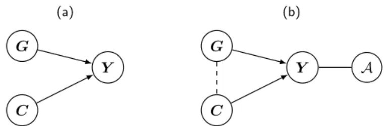
Assume that we are studying the potential association between a genetic variant (G) and a binary trait. Furthermore, assume we have also measured environmental

or clinical covariate (C) associated with the trait but independent of the variant of

interest in the source population, so it is not a confounder (Figure 1.1). In this case

X = (G,C). If we ascertain a random sample of study subjects, then the variant

of interest and covariate will remain independent (Figure 1.1.a). Thus, the most powerful model for assessing association between the genetic variant and the binary trait includes the environmental covariate in a logistic regression model [Robinson and Jewell, 1991; Neuhaus and Jewell, 1993; Neuhaus, 1998; Pirinen et al., 2012], that is

P(Y|G,C) =logit−1(α0+α1G+α2C),

whereGis the genetic variant,C is the environmental covariate,α1 is the log odds ratio reflecting the impact of one additional allele of a SNP on disease risk andα2 is the log odds ratio reflecting the impact of one additional unit ofCon disease risk.

(a)

G

C

Y

(b)

G

C

Y A

Figure 1.1: Example to illustrate possible correlation structures among risk factors and a trait in (a) a random sample and (b) a case-control sample. G:

SNP, C: clinical or environmental covariate, Y: binary disease trait, A: ascertainment. Continuous arrows between two nodes connect variables that could be correlated in the population while dashed lines represent induced correlations due to ascertainment.

2012]. Fortunately, using the retrospective likelihood approach in (1.3) one can address this problem by explicitly imposing the independence assumption between the genetic variant and the covariate [Umbach and Weinberg, 1997; Chatterjee and Carroll, 2005], that is

Lr(α,β) =P P(Y|G,E)P(G)P(E) G∗_,E∗P(Y|G∗,E∗)P(G∗)P(E∗)

.

It is known that the phenotype of an organism is sometimes determined, not only by its own genotype and environment, but also by the environment and genotype of its parents. Examples of such situation are maternal effects, i.e. when an organism shows the phenotype expected from the genotype of the mother, irrespective of its own genotype. Other examples of such situations are the non-inherited maternal antigen effects (NIMA), i.e. antigens passed from the mother to the offspring during pregnancy, which increase or decrease the disease risk of an offspring. To capture such effects, model (1.4) can be extended to incorporate maternal genotype information,

g{E(Y|Gc, Gm)}=α0+α1Gc+α2Gm+α3f(Gc, Gm),

where Gc _{and G}m _{are the genotypes of the child and mother; α}

1 andα2 are their effects on disease risk of the child; f(Gc_{, G}m_{)is a function that takes into account} the different offspring-mother genotype combinations that can result in a NIMA effect with

f(Gc, Gm) =

(

1 if Gm, but notGc , increases or decreases disease risk,

0 if Gm _{, does not increase or decrease disease risk.} ,

andα3 is the NIMA effect.

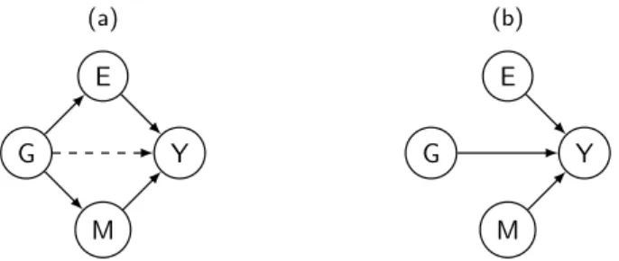
The two factors we try to bridge in genetic association studies are SNPs and disease risk. While this approach has successfully identified many associations, the biological mechanisms underpinning the change in risk remain often unknown. Inter-mediate cellular phenotypes, such as gene expression and DNA methylation, which are now being collected in addition to genetic data, provide an opportunity to address this issue. Performing joint analysis over these multiple data types (i.e. integrative omics) has advantages for both biological and statistical reasons. For example, gene expression and DNA methylation can help explain variability of the effect of the SNP on disease when the effect of the SNP on disease is mediated via gene expression and/or DNA methylation, illustrated in Figure 1.2.a, or they can help remove un-wanted variation from the phenotype when each variable has an independent effect on disease risk, illustrated in Figure 1.2.b. In both cases this will increase the power of detecting the overall effect of SNPs on disease risk.

1.4

This thesis

1.4. THIS THESIS 9

(a)

G E

M Y

(b)

G E

M Y

Figure 1.2: Example to illustrate possible correlation structures among a binary disease trait (Y) and the omics risk factors. The omics risk factors are a SNP (G),

a gene expression measurement (E), and a DNA methylation measurement (M). (a) The effect of G on Y is mediated via E and/or M and (b) Each of E, M, and G have an independent effect on Y. Continuous arrows between two nodes connect variables that could be correlated in the population while dashed lines represent mediation effect.

thesis is to construct statistical methods that use “richer" models for the relation-ship between the genetic variants and the phenotype, compared to models used in standard genetic association studies, incorporate information from both family and case-control based studies; different types of data; genetic, genomic, epigenomic and environmental information; and allow the genetics community to answer more complicated questions about the genetic architecture behind complex traits. Each Chapter is based on a paper, already published, submitted or prepared for submission, that addresses different issues of genetic association studies and current studies of the genetic basis of human disease. In the next section we present these problems and the solutions we propose.

Chapter 2 describes a novel method to improve the power of GWAS by combining data from multi-case family studies and twin studies. To maximise efficiency in parameter estimation we base the inference about the parameters of interest on an ascertainment-corrected joint likelihood. To take into account the correlation of disease risks among family members, due to shared but unmeasured genetic or environmental factors, we use a family-specific random term. We show in both simulated and real data that this families and twins combined ascertainment-corrected joint likelihood approach is more efficient for estimating the parameters of interest, as compared to a families-only approach or a prospective approach which ignores the ascertainment.

many realistic scenarios, as compared to single SNP-based and standard haplotype-based studies.

Chapter 4 investigates the contributions that linkage-based methods, such as identical-by-descent mapping, can make to association mapping to identify rare vari-ants in next-generation sequencing data. Linkage mapping methods are more pow-erful for identifying highly penetrant variants with low frequencies while association mapping methods are more suitable for identifying more common variants with mod-erate effect sizes. The hope is that, by combining both methods, we would be able to identify variants with moderate effect sizes and moderate to low frequencies. We ap-ply the method to next-generation sequencing longitudinal family data from Genetic Association Workshop 18.

Chapter 5 introduces a novel statistical method to improve the power of GWAS and further characterize genetic mechanism behind complex diseases by using integra-tive omics. Recent works on integraintegra-tive omics use prospecintegra-tive approaches, modelling case-control status conditional on omics and non omics risk factors. In this chapter, we propose a novel statistical method for integrating multiple omics and non-omics factors in case-control association studies based on a retrospective likelihood func-tion, which accounts for the ascertainment present in the case-control data. The new method has increased efficiency over prospective approaches in both simulated and real data.

2

Combining Family and Twin Data in

Association Studies

1

Summary

It is hypothesized that certain alleles can have a protective effect not only when inher-ited by the offspring but also as non-inherinher-ited maternal antigens (NIMA). To estimate the NIMA effect, large samples of families are needed. When large samples are not available, we propose a combined approach to estimate the NIMA effect from ascer-tained nuclear families and twin pairs. We develop a likelihood-based approach allow-ing for several ascertainment schemes, to accommodate for the outcome-dependent sampling scheme, and a family-specific random term, to take into account the cor-relation between family members. Simulations show that the combined likelihood is more efficient for estimating the NIMA odds ratios as compared to a families-only ap-proach. To illustrate our approach, we used data from a family and a twin study from the United Kingdom on rheumatoid arthritis, and confirmed the protective NIMA ef-fect, with an odds ratio of .477 (95%CI .264-.864). The method is publicly available

athttps://github.com/BrunildaBalliu/NIMA.

2.1

Introduction

Genetic studies typically focus on testing whether a genetic variant is associated with disease risk directly through the genotype of the offspring, i.e. offspring allelic effect, to identify susceptibility genes involved in complex disorders. However, many genes influence disease susceptibility through more complex biological mechanisms, such as conditions during embryonic or fetal life. One such mechanism, the non-inherited

1_{Published inGenetic Epidemiology.}

maternal antigens (NIMA) effect, may be involved in the pathogenesis of certain autoimmune diseases, such as rheumatoid arthritis (RA) [Hsieh et al., 2007; Feitsma et al., 2007], renal graft survival [Smits et al., 1998], and scleroderma [Nelson et al., 1998; Azzouz et al., 2011]. The NIMA effect affects disease susceptibility through a specific maternal-offspring genotype combination, i.e. the mother carries the allele of interest but the offspring does not. When the NIMA effect is present and not correctly modeled it can result in biased estimates of the offspring allelic effect [Weinberg, C. R., 1999; Sinsheimer et al., 2003].

In order to investigate such mechanisms, ascertained multi-case family designs are typically used. They are known to improve efficiency when studying the associ-ation of a disease with low prevalence and a low frequency variant, as compared to case-control studies of unrelated individuals [Kraft and Thomas, 2000]. To accom-modate for potential residual correlation in disease risks among family members, due to shared but unmeasured genetic or environmental factors, mixed models with family specific random terms are used. An ascertainment correction is needed to account for the outcome-dependent sampling schemes, often used to increase efficiency when studying a disease with low prevalence.

Several methods have been developed to model and/or test for the NIMA effect [Hsieh et al., 2006; Feitsma et al., 2007]. However, these methods are not appropriate for families that contain both multiple cases and healthy siblings. Feitsma et al. [2007] use information only from one affected offspring per family. Hsieh et al. [2006] take into account information from multiple affected siblings, but the correlation between disease outcomes among family members, is ignored. Ignoring this correlation may have an effect on the ascertainment correction, resulting in biased results for both standard errors and effect sizes [Kraft et al., 2005; Hsieh et al., 2006]. Both methods ignore the information available from healthy siblings by excluding them from the analysis.

Recruiting, genotyping, and interviewing members of multi-case families can be difficult due to the lack of clear sampling definition and the high cost, resulting in data sets with small sample size, thus low power to detect the effect of interest. To enhance the statistical power to identify disease susceptibility genes, Pfeiffer et al. [2008] and Zheng et al. [2010] proposed to combine family-based studies with case-control studies using a prospective likelihood (P L) approach, modelling the distribution of the phenotypes of family members conditional on their genotypes. These methods focus on direct effects, and as expected, due to the larger sample size, they increase the power to detect the direct offspring allelic effect [Pfeiffer et al., 2008; Zheng et al., 2010]. Typically, studies with multi-case families lack power to estimate the effects of rare protective factors, such as the NIMA effect. To address this problem, we propose to combine the multi-case family study with a twin-based study and use the joint likelihood (J L), which models the joint genotype and phenotype distribution, instead of theP L. TheJ Lcan be more efficient for estimating the genetic odds ratios since it only conditions on the ascertainment event, and uses information from the modelling the genotype distribution of the parents and offspring [Kraft and Thomas, 2000].

2.2. MATERIAL AND METHODS 13

the direct protective effect from both family and twin likelihood and the indirect NIMA effect from the family likelihood. In a similar way, Chen et al. [2012] use a semi-parametric likelihood where the environmental effect is treated as a nuisance parameter. By combining families with a twin study, as compared to a case-control study, we have more information on familial genotypes distribution, by assuming Mendelian inheritance, random mating and HWE.

The disease of interest in this article is RA, a genetic disorder in which alleles of the HLA-DRB1 gene contribute most to the genetic risk. A group of alleles in this gene, called DERAA alleles, are known to have a protective effect against RA, when present in the genotype of the offspring. Recent observations suggest that bio-logically relevant exposure to HLA-antigens may occur during fetal development and subsequently through the persistence, of maternal cells in the offspring. This phe-nomenon is called micro-chimerism. It has been proposed that not only inherited but also non-inherited maternal HLA-antigens can influence RA susceptibility [Feitsma et al., 2007]. This implies that the exposure of DERAA-negative offspring to ma-ternal DERAA-positive HLA-DRB1 antigens during fetal development might have a protective effect on the offspring. We applied the combined joint likelihood (CJ L) to 94 multi-case RA nuclear families [Hay et al., 1993; Worthington et al., 1994] and 78 dizygotic twin pairs [Silman et al., 1993], both collected from the National Repository of Family Material of the Arthritis and Rheumatism Council’s.

Our method is a general framework for family-based association analysis, incor-porating the advantages of several previously proposed methods such as combining different data sets, likelihood-based modelling, ascertainment correction and model-ing correlation between disease outcome of siblmodel-ings.This novel method models the joint genotype and phenotype distribution, taking into account the ascertainment and correlation present in the data, and combines families and twins studies to in-crease information to estimate the NIMA effect. In the next sections we introduce the general idea of the CJ L for family-based and twin-based studies; we provide detailed estimation procedures for the family study and generalize the method to the twin study. The performance of our proposed method is assessed via an extensive simulation study and different approaches are compared for several scenarios, on the efficiency to estimate genetic odds ratios. The proposed method is illustrated with an analysis of the Arthritis and Rheumatism Council data.

2.2

Material And Methods

2.2.1

Notation and Data

Consider a study where information is available from two different data sets, a family-based and a twin-family-based study. For every family, genotype and phenotype information is available for the offspring, affected and/or healthy, and most of their parents. Families were ascertained on the event of at least two affected offspring per family. Genotypic and phenotypic information is also available for each twin, but not for their parents. Twin pairs were ascertained such that each pair contains at least one affected member.

LetYi= (Yi1, Yi2, ..., Yini)denote phenotypes or disease status ofnioffspring in

andj=1,...,ni. Similarly, let Gci = (Gci1, Gci2, ..., Gcini)denote the genotypes of the

ni offspring andGp_i = (Gm_i , Gf_i)their maternal and paternal genotypes. We denote

byNf andNt the total number of families and twin pairs respectively. Last, letAi be the ascertainment event for a family or twin pair.

2.2.2

Statistical Models

A commonly used approach for family data is the conditional logistic regression [Bres-low and Day, 1980]. It conditions on the number of observed cases in each family, to accommodate for the outcome-dependent sampling scheme, and uses a family specific random term, to account for dependencies in disease risk among siblings. When twins are also available, we propose to estimate the genetic odds ratios by maximizing the combined likelihood for families and twins, instead of a families-only approach. Under the assumptions that the data sets are sampled separately from the same population, with no overlap between them and with comparable data collection methods, the combined likelihood can be obtained by the product of the likelihoods for each independent study.

Likelihood for family-based study

To model the association between genotypes and phenotypes of family members we use theJ L. This approach is based on the joint probability of phenotypes and genotypes, that isP(Yi,Gci,G

p

i |Ai)and is given by:

J Lf(θ) =

Nf

Y

i=1

P(Yi,Gc_i,Gp_i |Ai), (2.1)

where θ is the parameter vector. P(Yi,Gc_i,Gp_i |Ai) for family i is defined as follows:

P 

Yi,Gci,G p i |

ni

X

j=1 Yij ≥2



=

PYi,Gc i,G

p i,

Pni

j=1Yij≥2

PPni

j=1Yij≥2

(2.2)

=P(Yi|G

c i,G

p

i)×P(G c i |G

p

i)×P(G p i) PPni

j=1Yij ≥2

.

The second identity of (2.2) requires two assumptions. First, subjects selection should depend only upon potential subjects’ disease status, not on their covariates, that is P   ni X j=1

Yij≥2|Yi,Gc_i,Gp_i



=P 

 ni

X

j=1

Yij ≥2|Yi 

.

Secondly, families should be selected under complete ascertainment, that is PPni

j=1Yij ≥2|Yi

= 1for a family with at least two affected offspring, and 0

2.2. MATERIAL AND METHODS 15

The numerator of (2.2) is a product of the disease penetrance function P(Yi |

Gc

i,G p

i), thetransmission probabilitiesP(Gci |G p

i)and theparental genotype prob-abilities P(Gp_i). The disease penetrance function models the disease probability of

ni offspring given the genotypes of the family. We will explain how we model the penetrance function in the next section. We assume Mendelian inheritance for the transmission probability P(Gc

i |G p

i), random mating for the parents and HWE for the genotype distribution. Thus, the parental genotype probability P(Gp_i) is

char-acterised by a single parameter, the allele frequencyq.

The denominator is theascertainment correctionand models the probability that at least two offspring in the family are affected. This probability can be expressed in terms of the marginal distribution by summing the joint distribution of phenotype and genotypes over all possible genotype combinations in a family, that is :

P   ni X j=1 Yij ≥2



= 1− X

Gc

∗,G

p

∗

P(Gc_∗|Gp_∗)×P(Gp_∗) (2.3)

×    P   ni X j=1

Yij= 1|Gc_∗,Gp_∗



+P 

 ni

X

j=1

Yij = 0|Gc_∗,Gp_∗

     .

Disease penetrance function

In this section we present the penetrance function for a family in the data set. Given a set of family-specific random effects ui, we assume that (Yi1, Yi2, ..., Yin_i) are

conditionally independent. Thus, the penetrance function for one family can be expressed as the product of the penetrance functions for each offspring in the family:

P(Yi|Gci,G p i, ui) =

ni

Y

j=1

P Yij =yij |Gcij,G p i, ui

.

In order to estimate the parameters of interest, we use the marginal probability of the disease outcome of theith family, given by:

P(Yi|Gci,G p i) =

Z

ui

P(Yi|Gci,G p

i, ui)f(ui)dui. (2.4)

We assume that the random intercept is normally distributed, ui ∼ N 0, τu2

. The integral is analytically intractable and we resort to numerical integration. To evaluate the integral we used the Gauss - Hermite Quadrature rule.

Last, we specify the individual penetrance function. We consider here the case where a direct offspring allelic effect and an indirect NIMA effect affect the disease probability for each offspring. We assume no direct maternal or paternal allelic ef-fect. The disease probability for each offspring is a function of offspring genotype, combination of maternal and offspring genotype and the random effectui:

P Yij = 1|Gc_ij,Gm_i , ui

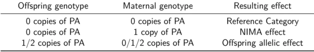
Table 2.1: Possible genotype combination of mother-offspring pair and resulting protective effects. PA: protective allele, NIMA: non-inherited maternal antigens.

Offspring genotype Maternal genotype Resulting effect 0 copies of PA 0 copies of PA Reference Category

0 copies of PA 1 copy of PA NIMA effect

1/2 copies of PA 0/1/2 copies of PA Offspring allelic effect

where logit−1 _{is the inverse logit function, logit}−1_{(x) =} exp(x)

1+exp(x). Parameter β0 is the intercept of the logistic model. Let I[.] denote an indicator function.

OAEij denotes an event of offspring allelic effect. We assume a dominant model, whereOAEij = 1 when one or two copies of the protective allele are present in the

offspring’s genotype and zero otherwise. Parameterβ1 represents the log odds ratio of disease probability for the offspring allelic effect. LetN IM Aij denote an event of NIMA, whereN IM Aij = 1if a copy of the protective allele is present in the maternal

genotype but not present in the offspring’s genotype and zero otherwise. Parameter β2represents the log odds ratio of the NIMA effect. The interpretation of parameters is conditional on the family specific random effects. In Table 2.1 all possible genotype combination of mother-offspring pair and resulting effects are reported.

Likelihood for twin-based study

In this section we modify the J L presented in the previous section to model data from twin-based studies. Since no parental genotypes are available in the twin study, it is not possible to estimate the indirect NIMA effect. Namely, the twin likelihood contains no information about NIMA. However, we need to include the NIMA pa-rameter in the twin likelihood to ensure that the papa-rameters of the family and twin likelihood have the same interpretation. Missing data is dealt with by marginalizing over all possible parental genotypes combinations, treatingβ2 as a nuisance param-eter. Following the notation used in (2.1), the J L for the twin data set is given by:

J Lt(θ) =

Nt

Y

i=1

P(Yi,Gc_i,|Ai), (2.6)

where P(Yi,Gc

i,|Ai)for twin pairiis given as follows:

P 

Yi,Gc_i | 2 X

j=1 Yij ≥1



= X

Gp∗

P 

Yi,Gc_i,Gp_∗| 2 X

j=1 Yij ≥1





=X

Gp∗

P(Yi|Gci,G m

∗)×P(Gci |G p

∗)×P(Gp∗)

1−P

Gc

∗,Gp∗P

P2

j=1Yij = 0|Gc∗,Gm∗

×P(Gc ∗|G

p

2.3. SIMULATION STUDY 17

Combined likelihood for the family and twin studies

To obtain joint estimates for the NIMA and direct offspring allelic effect we maximize the combined likelihood for both data sets, given by the product of the likelihood contribution from family study (2.1), and the likelihood contribution from twin study (2.6):

CJ L(τu, β0, β1, β2) =J Lf(τu, β0, β1, β2)×J Lt(τu, β0, β1, β2). (2.7) Information to estimate the direct allelic effect, the baseline risk and the variance of the random effect comes both from twins and families. On the other hand, the family likelihood allows us to estimate also the NIMA effect. By adding the twins to the families, we borrow information to better estimate the direct allelic effect, which will also improve the estimate of the NIMA parameter through the family likelihood.

2.3

Simulation Study

The primary goal of the simulation study was to test efficiency gain for estimating effects that depend on parental genotype, such as NIMA, when a twin data set, with missing parental information, is combined with a data set comprised of nuclear families. In addition, we wanted to study the finite sample properties of the J L itself and relative to theP L. In particular, we investigated the impact of family size, variance of random effects and ascertainment scheme on the parameter estimates, and compared our method with theP Lused in previous studies, in terms of efficiency and bias of estimates of NIMA effect.

In each scenario, genotype frequencies were selected to mimic the frequency of DERAA alleles in the English population, i.e. .15 [Ann Morgan, personal communi-cation]. To generate genotypes of family members, maternal and paternal genotypes were generated assuming random mating and HWE. Offspring genotypes were gener-ated assuming Mendelian transmission. Disease outcomes of offspring were genergener-ated according to the random effects model (2.5). The family-specific random intercept was assumed to be normally distributed with mean zero and variance either 1.5 or 2.5, resembling results from previous literature on heritability of RA [van der Woude et al., 2009]. Two different ascertainment schemes were used, that is, families were included in the study if at least one or two offspring were affected. Twins were generated as families with two offspring, ascertained such that at least one twin per pair is affected. Parental genotype and phenotype information was ignored to mimic the real data set. We set β0 to -3, representing a common disease with population prevalence approximately 5%. The true parameter values for offspring allelic and

NIMA effect, β1 and β2, were fixed at -.5 and -1, corresponding to an odds ratio of .6 and .4 respectively. In total, 16 scenarios were generated, each consisting of

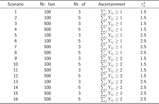
103 _{simulated data sets, with corresponding family and sample size, ascertainment} scheme and variance of the random effect as indicated in Table 2.2.

Table 2.2: Simulation scenarios with varying sample and family size, ascertainment scheme and variance of the random effects. fam: family, of: offpsring, P

jYij ≥1: at least one affected offspring, P

jYij ≥ 2: at least two affected offspring, τu2: variance of random effect.

Scenario Nr. fam Nr. of Ascertainment τ2

u

1 100 3 P

jYij ≥1 1.5

2 100 5 P

jYij ≥1 1.5

3 500 3 P

jYij ≥1 1.5

4 500 5 P

jYij ≥1 1.5

5 100 3 P

jYij ≥1 2.5

6 100 5 P

jYij ≥1 2.5

7 500 3 P

jYij ≥1 2.5

8 500 5 P

jYij ≥1 2.5

9 100 3 P

jYij ≥2 1.5

10 100 5 P

jYij ≥2 1.5

11 500 3 P

jYij ≥2 1.5

12 500 5 P

jYij ≥2 1.5

13 100 3 P

jYij ≥2 2.5

14 100 5 P

jYij ≥2 2.5

15 500 3 P

jYij ≥2 2.5

16 500 5 P

2.3. SIMULATION STUDY 19

resulting in an underestimatedβ0. However, estimates of the log odds ratios for the offspring allelic and NIMA effect are nearly unbiased, -2.3% and 3.4% respectively.

Increasing family size from 3 to 5, scenario 2, reduces the bias of both effects to .1%

and 2.4% and their standard deviations by 8.5% and 11.43% respectively. On the

other hand, increasing the number of families from 100 to 500, scenario 3, reduces the bias of both effects to -1.4% and -1.0%and their standard deviations by 55.6%and

58.4% respectively. To study the effect of differentτ2

u on the parameter estimates, we compared scenarios 1-4 with scenarios 5-8 or/and scenario’s 9-12 with scenarios 13-14. Whenτ_u2increases from 1.5 to 2.5, from scenario 1 to scenario 5, bias on the estimate ofβ0andτu2itself increases. However, this does not introduce much bias in the estimation of the offspring allelic and NIMA parameters. Different ascertainment schemes were compared by contrasting scenarios 1-4 with scenarios 9-12. Bias in τ2

u andβ0 estimates increases when ascertainment is PjYij ≥ 2, as compared to P

jYij ≥ 1 while estimates of the offspring allelic and NIMA parameters remain unbiased, e.g. bias in scenario 9, forβ1 andβ2, is 1.9%and 5.7% respectively.

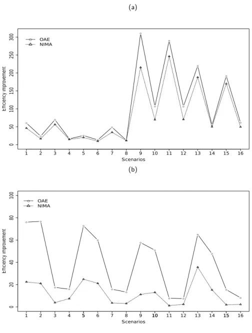
Next, we compare the two different likelihoods to model family/twin data in terms of efficiency, the P Lused in existing methods, with the approach we use in this article, theJ L. We define the percentage of efficiency improvement of likelihood A over B, for estimating a parameterβ, as EI= (1−V ar(βA)

V ar(βB))×100. Positive values

mean that likelihood A performs better. In Figure 2.1.a we plot the EI of theJ Lover theP L, for estimating the log odds ratios of the offspring allelic and NIMA effect. All values are positive, thus the J L is always more efficient. Improvement mainly depends on sample size and less on family size, e.g. EI is approximately the same in scenario 1 and 3 as compared to scenario 2. Moreover, improvement, due toJ L, is higher when information is limited, i.e. when families are small and ascertainment is P

jYij ≥2.

Last, we compared the performance of the J L when different data sources are available: ascertained families-only versus ascertained families and twins. In terms of likelihoods, we compare the J L in (2.1) with the CJ Lin (2.7). Efficiency im-provement of the families-only against the combined approach, with families and 100 twin pairs, is plotted in Figure 2.1.b. TheCJ Lapproach is more efficient under all scenarios studied. The percentage of improvement is similar across different values of variance of the random effects or ascertainment scheme. Nonetheless, improvement is noticeably high when the sample size of the nuclear family data is small. When the twin data set was added, we expected efficiency improvement for the offspring allelic effect, due to increased sample size. Interestingly, there was also efficiency improvement for the NIMA effect, which depends on the maternal genotype. The parameter estimates and their standard deviations, using theCJ L, are listed in Table A.2.1 of the Appendix.

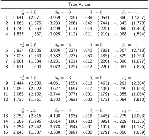
In order to asses the performance of our method when both direct offspring and NIMA effects are under the null,β1=β2= 0, and cases in which there only exists a

direct offspring,β2= 0, or only a NIMA effect,β1 = 0, we simulated the scenarios

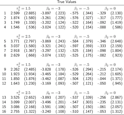
Table 2.3: Summary statistics for parameter estimates of the J L (2.1) under the penetrance model (2.5) for each scenario described in Table 2.2. Each entry lists the mean estimates (standard deviation of estimates) over 1000 simulated data sets. JL: joint likelihood.

True Values

τu2= 1.5 β0=−3 β1=−.5 β2=−1 1 2.148 (2.538) -3.365 (1.460) -.477 (.349) -1.034 (.507) 2 1.584 (1.038) -3.049 (.579) -.501 (.319) -1.024 (.449) 3 1.571 (.771) -3.052 (.466) -.486 (.155) -.990 (.211) 4 1.543 (.411) -3.022 (.226) -.497 (.140) -1.000 (.197)

τ2

u = 2.5 β0=−3 β1=−.5 β2=−1 5 3.517 (3.382) -3.476 (1.612) -.478 (.397) -1.016 (.541) 6 2.724 (1.662) -3.104 (.766) -.503 (.344) -1.022 (.469) 7 2.587 (1.152) -3.045 (.572) -.492 (.169) -1.001 (.231) 8 2.577 (.629) -3.033 (.290) -.504 (.149) -1.003 (.196)

τ2

u = 1.5 β0=−3 β1=−.5 β2=−1 9 2.827 (3.001) -4.236 (2.864) -.519 (.265) -1.057 (.407) 10 1.980 (1.765) -3.408 (1.442) -.501 (.258) -1.020 (.386) 11 2.472 (2.290) -3.929 (2.194) -.499 (.120) -.999 (.173) 12 1.607 (.672) -3.091 (.560) -.497 (.112) -.994 (.167)

τ2

2.3. SIMULATION STUDY 21

(a)

●

● ●

● ●

● ●

● ●

● ●

● ●

● ●

●

5 10 15

0

50

100

150

200

250

300

Scenarios

Efficiency impro

vement

1 2 3 4 6 7 8 9 11 12 13 14 16

● OAE

NIMA

(b)

● ●

● ●

●

●

● ●

●

●

● ●

●

●

●

●

5 10 15

0

20

40

60

80

100

Scenarios

Efficiency impro

vement

1 2 3 4 5 6 7 8 9 10 11 12 13 14 15 16

● OAE

NIMA

The performance of our approach will vary across different frequencies of the protective allele. All the results presented above concern an allele frequency of .15, in order to mimic the allele frequency in the population we are studying. To study the performance of the method when allele frequency is lower, we also applied the CJ L to samples generated with a protective allele frequency of .05. As expected, the parameter estimates are more biased for small sample sizes. Larger samples are needed to obtain unbiased estimates. Results are listed in Table A.2.7 of the Appendix.

2.4

Data Example

This study was motivated by a data set consisting of 94 ascertained nuclear families, collected from the Arthritis and Rheumatism Council. Our goal is to study the effect of NIMA in RA susceptibility. In 51 families the genotype of one of the parents, mainly the father, was missing. In 34 families, of which 8 had a missing mother and 26 a missing father, we were able to construct the genotypes using the genotypes of the offspring and the genotype of the other parent. Namely, we reconstructed the missing genotype in accordance with Mendelian transmission law. For the remaining 17 families, of which 9 were mothers and 8 were fathers, we were able to reconstruct only one of the alleles using this approach. In order to impute the second allele, we made use of the initial 4-digit allele coding of the HLA-DRB1 gene. There are 26 possible 4-digit sequences in the HLA-DRB1 gene, six of which express this DERAA allele, see van der Woude et al. [2010]. We imputed the second allele based on sampling from control 4-digit allele distribution. For 6 out of 9 mothers we had only the first 2 digits of the 4-digit genotyping and for the rest 3 we had no information about the second allele.

Families mainly contain two, three and four offspring. There are also three large families with five, eight and ten offspring. 86 families out of 94 contain exactly two affected offspring and 8 families contain three affected offspring. The maternal-offspring genotype combination that leads to the potential NIMA effect occurs only in 8 families. In these 8 families, 4 have one child, 2 have two children and 2 have three children under potential NIMA effect. In addition, 20 offspring belonging to 13 families are under offspring allelic effect. Since there is so little information in the family data set, we decided to combine it with a data set of 78 ascertained twin pairs, also collected from the Arthritis and Rheumatism Council in the same period. Pairs mainly contain one affected member and only in 3 pairs both members are affected. In 4 pairs both twins carry the DERAA allele, DERAA-concordant, while in 10 pairs only one twin has the allele, DERAA-discordant. In total, 18 twins are under offspring allelic effect. Information on parental genotype of twins is not available, thus the exact number of twins under a possible NIMA effect cannot be determined. Initially, we only analyzed the family data, using both the J L and the P L ap-proach. Results are listed in the first two lines of Table 2.4. None of the likelihoods gave statistically significant results for the NIMA effect, estimated odds ratios .176 (95% C.I. .010-3.066) and .607 (95% C.I. .348 1.058) for the P Land the J L ap-proach respectively. Concerning the offspring allelic effect, only the J L resulted in a statistically significant result, odds ratios .194 (95% C.I. .023-1.622) for the

2.5. DISCUSSION 23

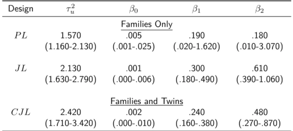
Table 2.4: Parameter estimates (95%C.I.) of the disease penetrance model (2.5) by

types of likelihood approaches used, prospective (P L), joint (J L), or combined joint likelihood (CJ L), and type of data included, families only or families and twins.

Design τ2

u β0 β1 β2

Families Only

P L 1.570

(1.160-2.130) (.001-.025).005 (.020-1.620).190 (.010-3.070).180

J L 2.130

(1.630-2.790) (.000-.006).001 (.180-.490).300 (.390-1.060).610

Families and Twins

CJ L 2.420

(1.710-3.420) (.000-.010).002 (.160-.380).240 (.270-.870).480

we combined the families with the twins and applied the CJ L. The odds ratio of the NIMA effect was statistically significant, .477 (95% C.I. .264-.864) and the

con-fidence intervals of the odds ratios of the offspring allelic effect became narrower; .241 (95% C.I. .152-.380).

To conclude, we estimated a significant protective effect of the DERAA allele, coming directly from the genotype of the offspring and indirectly from the maternal genotype. That is, individuals carrying the DERAA allele have a decrease in risk of RA compared to individuals who do not carry it. Furthermore, individuals who do not carry the protective allele DERAA, but their mother does, have a decrease in risk to develop RA as compared to non-DERAA carriers whose mother also does not carry the protective allele.

2.5

Discussion

be-tween phenotype of siblings using an ascertainment correction and a family-specific random effects model.

Our approach extends existing methods for combining data sets [Pfeiffer et al., 2008; Zheng et al., 2010] to include indirect effects, using a J L, instead of a P L approach and adding twins, instead of a case-control data set. We compared the proposedJ Lmethod with the traditionally usedP Lapproach and showed that our method is more efficient for estimating the genetic odds ratios, especially for small families with stringent selection schemes. For prospective or joint likelihood methods, including ours, ascertainment correction is essential to obtain unbiased parameter estimates. Here, we considered cases for which subjects’ selection depends only upon potential subjects’ disease status and not on their covariates. When ascertainment is also based on covariates, here genotypes, another model for ascertainment correction should be considered.

Using the J L, power can considerably increased, however at the cost of greater computational intensity, in the presence of large families. In our data set, the families where relatively small and numerical optimization of theJ Lwas possible on a single computer. However, in the presence of large families, the computational burden rises exponentially with the family size. For given parameter values and allele frequency, the denominator (2.3) for familyisums over maximum3nipossible familial genotype

combinations. If all the families in the data set have a fixed size, the denominator needs to be calculated onlyptimes for each maximization iteration, wherepis the number of sample points to use for the Gauss-Hermite Quadrature approximation of the integral (2.4). Unfortunately, this is rarely the case in real data sets where the family size varies but the computation burden can be essentially reduced by using a grid search.

Here, we combine a family data set with a twin data set. However, the method can be extended to include other types of readily available data, such as sibling-pairs, monozygotic twins, or case-parent trios data sets. Nowadays, the combination of already available data is facilitated from existing nationwide registries of families and twins at high risk for particular traits. Extension of the likelihood-based analysis described here, to accommodate multi-allelic marker, is trivial, if HWE and random mating assumptions are made. Although we have focused on association of single SNPs, the approach can be extended to allow for the analysis of haplotypes. Since haplotypes combine linkage disequilibrium information from multiple markers simul-taneously, this approach could be more powerful than our current approach. Direct extension to accommodate haplotypes is not straightforward, due to the increase in the number of parameters needed to model the haplotypes, and is beyond the scope of this article. The proposed method can be extended to other complex biologi-cal mechanisms, such as maternal effects or imprinting, by adding the appropriate covariates in the logistic regression (2.5). Last, by incorporating our method to methodology applied in Houwing-Duistermaat et al. [2000], we could study whether genetic NIMA effects of RA could create a protection for diseases associated with RA, such as cardiovascular disease or anaemia.

2.5. DISCUSSION 25

underlying random effects distribution [Heagerty and Kurland, 2001; Pfeiffer et al., 2003]. One could also analyze the data simply by using a GEE approach [Liang and Zeger, 1986]. However, since the GEE estimates do not take into account the sampling design, the resulting covariate effect estimates might be biased, because the family and twin data sets are not a random sample of the families and twins in the population. While the random effects model allows one to accommodate ascertainment of the families as well as residual familial correlation, the interpretation of the parameters is conditional on the random effects [Fitzmaurice et al., 1993]. Marginal parameter estimates can be obtained using the approximate formula of Diggle et al. [1994]. This approximation uses the variance of the random effects. In the simulation study we observed that the estimate of the variance, needed for the marginalization, might be biased when sample size is small. Thus we recommend to use the approximation formula only when the sample size and/or family size are large, e.g. 500 families with 3 offspring when ascertainment is at least one affected offspring.

2.6

Appendix

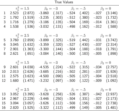
Table A.2.1: Summary statistics for parameter estimates of the CJ L when both direct genetic and NIMA effect are present, for each scenario in Table 2.2. Each entry lists the mean estimates (standard deviation of estimates) over 1000 simulated data sets.

True Values

τu2= 1.5 β0=−3 β1=−.5 β2=−1 1 2.211 (2.511) -1.391 (1.467) -.508 (.263) -1.104 (.458) 2 1.613 (.966) -1.052 (.552) -.517 (.240) -1.080 (.408) 3 1.588 (.779) -1.057 (.472) -.492 (.143) -1.007 (.207) 4 1.547 (.403) -1.021 (.223) -.502 (.130) -1.013 (.190)

τ2

u = 2.5 β0=−3 β1=−.5 β2=−1 5 3.558 (3.193) -1.503 (1.596) -.514 (.302) -1.091 (.484) 6 2.749 (1.559) -1.103 (.742) -.525 (.272) -1.083 (.426) 7 2.608 (1.151) -1.051 (.574) -.499 (.157) -1.018 (.227) 8 2.581 (.617) -1.032 (.287) -.509 (.140) -1.017 (.193)

τ2

u = 1.5 β0=−3 β1=−.5 β2=−1 9 2.394 (2.403) -1.645 (1.770) -.509 (.211) -1.088 (.386) 10 1.934 (1.594) -1.320 (1.177) -.511 (.210) -1.065 (.363) 11 1.937 (1.495) -1.386 (1.315) -.499 (.112) -1.009 (.172) 12 1.606 (.634) -1.084 (.511) -.500 (.108) -1.005 (.165)

τ2