AENSI Journals
Australian Journal of Basic and Applied Sciences
ISSN:1991-8178
Journal home page: www.ajbasweb.com
Corresponding Author: Woan-Lin Beh, Universiti Tunku Abdul Rahman, Department of Physical and Mathematical Science, Faculty of Science, 31900 Kampar, Perak, Malaysia.
Ph: (+60)16-4420515. E-mail: [email protected].
Pricing of American Call Options Using Regression and Numerical Integration
1W.L. Beh, 2A.H. Pooi, 3K.L. Goh
1Universiti Tunku Abdul Rahman, Department of Physical and Mathematical Science, Faculty of Science, 31900 Kampar, Perak, Malaysia 2Sunway University Business School, 47500 Subang Jaya, Selangor, Malaysia.
3University of Malaya, Department of Applied Statistics, Faculty of Economics and Administration, 50603 Kuala Lumpur, Malaysia.
A R T I C L E I N F O A B S T R A C T
Article history:
Received 30 September 2014 Received in revised form 17 November 2014 Accepted 25 November 2014 Available online 13 December 2014
Keywords:
American option pricing, simulation, numerical integration, Levy process, regression, N-dimensional polar coordinate system
Consider the American basket call option in the case where there are N underlying assets, the number of possible exercise times prior to maturity is finite, and the vector of N asset prices is modeled using a Levy process. A numerical method based on regression and numerical integration is proposed to estimate the price of the American option. In the proposed method, we first express the asset prices as nonlinear functions of N uncorrelated standard normal random variables. For a given set of time-t asset prices, we next determine the time-t continuation value by performing a numerical integration along the radial direction in the N-dimensional polar coordinate system for the N uncorrelated standard normal random variables, expressing the integrated value via a regression procedure as a function of the polar angles, and performing a numerical integration over the polar angles. The larger value of the continuation value and the time-t immediate exercise value will then be the option value. The time-t option values over the N-dimensional space may be represented by a quadratic function of the radial distance, with the coefficients of the quadratic function given by second degree polynomials in N-1 polar angles. Partitioning the maturity time T into k* intervals of length Δt, we obtain the time-(k-1)Δt option value from the time-kΔt option values for k
= k*, k*-1,…, 1. The time-0 option value is then the price of the American option. It is found that the numerical results for the American option prices based on regression and numerical integration agree well with the simulation results, and exhibit a variation of the prices as we vary the non-normality of the underlying distributions of the assets. To assess the accuracy of the computed price we may use estimated standard error of the computed American option price. The standard error will help us gauge whether the number of selected points along the radial direction and the number of selected polar angles are large enough to achieve the required level of accuracy for the computed American option price.
© 2014 AENSI Publisher All rights reserved. To Cite This Article: Beh, W.L., A.H. Pooi and K.L. Goh, Pricing of American Call Options Using Regression and Numerical Analysis. Aust. J. Basic & Appl. Sci., 8(24): 8-17, 2014
INTRODUCTION
A major characteristic of the American option is that it can be exercised prior to maturity date. Pricing of American option is known to be a difficult problem especially when the number of underlying assets is large. The approaches for pricing American options include Monte Carlo simulation (Fu et al., 2001; Rogers, 2002), regression procedure (Carriére, 1996; Longstaff and Schwartz, 2001; Tsitsiklis and Van Roy, 1999, 2001), parametric approach (Bossaerts, 1989; Li and Zhang, 1996; Grant et al., 1997; Andersen, 2000; Garcia, 2003), stratification approach (Tilley, 1993; Barraquand and Martineau, 1995; Raymar and Zwecher, 1997), simulated tree approach (Broadie and Glasserman, 1997; Broadie et al., 1997b), neural networks (Hunt et al., 1992; Sanner et al., 1992; Kelly, 1994; Morelli et al., 2004; Kohler et al., 2006; Kohler and Krzyzak, 2009), and stochastic mesh method (Broadie and Glasserman, 1997; Avramidis and Hyden, 1999; Avramidis and Matzinger, 2004; Liu and Hong, 2009).
Let Si(t) be the time-t price of the i-th asset and S(t) = [S1(t), S2(t),…, SN(t)]
T
the vector of asset prices. In this study, we aim to estimate the American option price when there are N underlying assets, the possible exercise times prior to maturity are 0 = t0, t1, t2, …, tk* = T where tk = kΔt and Δt is a small increment in time,
To find the option value at S(tk), 0kk*-1, we express the vector S(tk+1) of prices at time tk+1 given the value S(tk) as a function of the vector e(k+1) = ( , ,..., )
) 1 ( ) 1 ( 2 ) 1 ( 1
k
N k k
e e
e of a set of uncorrelated standard normal random variables. The space formed by e(k+1) is next transformed to the N-dimensional polar coordinate system. The continuation value at S(tk) is computed by performing numerical integration along the radial direction and
over the polar angles. The option value at S(tk) is then given by the larger value of the time-t immediate exercise
value and the continuation value at S(tk).
To express the time-t option values over the N-dimensional space as an N-dimensional function, we first derive the distribution of S(tk) given S(t0). It turns out that the random vector S(tk) can be expressed as a function
of the vector ~e(k)=(~e1(k),~e2(k),...,~eN(k)) of another set of uncorrelated standard normal random variables. The space formed by ~e(k) is next transformed to an N-dimensional polar coordinate system. We approximate the time-t option values for the points along the radial direction by a low degree polynomial. By using a regression procedure, each of the coefficients of the polynomial in terms of the radial distance is next expressed as a low degree polynomial of the N-1 polar angles. In this way, we obtain the N-dimensional function which maps S(tk)
to the time-kΔt option value Q(tk, S(tk)). This function can then be used to find the option value at S(tk-1). As the option values are approximated by polynomials obtained by a regression procedure, the computed American option price would not be exact. We estimate the standard error of the option value at time tk for k =
k*-1, k*-2,…, 0 in the indicated order. The estimated standard error at t0 will then be an estimate of the standard error of the American option price.
When N is large, instead of paying the high cost of estimating the standard errors for all the values of k in {k*-1, k*-2,…, 0}, we may compute the initial few standard errors and use an extrapolation procedure to get an idea of the size of the standard error of American option price.
The layout of this paper is as follows. The method based on regression and numerical integration for pricing the American call options and the estimated standard error of the American option price will be discussed in details in next topic accordingly. The results will be presented in the Results and Discussion section. Meanwhile the conclusion will be given in the last section of this paper.
Pricing of American Call Options on the N Assets Using Regression and Numerical Integration:
Consider an American basket call option on the N assets (N ≥ 2) with time T to expiration and a strike price of K. Suppose the distribution of the vector of asset prices S(t) is described via a Levy process. The prices of the assets are usually correlated and each of them has fatter tails and thinner waist than the normal distribution. The multivariate normal distribution is thus not suitable for approximating the joint distribution of asset prices. In what follows, we approximate the distribution of the asset prices by using the quadratic-normal distribution which is introduced in Pooi (2003). To form the quadratic-normal distribution with parameters 0 and λi, we may begin with the following non-linear transformation
0 )),
2 1 ( ] [ (
0 )),
2 1 ( ] ([ ~
3 2
3 2 1
3 2
2 1
e e
e
e e
e
(1)
where ~e N(0, 1). If e has the standard normal distribution with the transformation in Eq.(1) is one-to-one, then
~is said to have the quadratic-normal distribution. The i-th component of the time-tk value of the vector of asset
prices S(tk)may be approximated by
t S S S t S w tSi k i(k) i(k1) i(k1)i i(k1)i i(k) , i = 1, 2,…, N, k = 0, 1,…, k* (2) where i and i are respectively the mean rate and volatility of the price of asset i and w(k) = (w1 k ,w2 k ,…,w Nk ) is a set of N random variables that has a correlation structure specified by the correlation matrix P = {ij} with ij = corr(wi k ,w jk ), for ij, i, j = 1, 2,…, N and ii= var(wi k ) = 1, for i = 1, 2,…, N. Let B = {bij} be the (NxN) matrix formed by the N eigenvectors of the (NxN) matrix P = {ij } and
) ( )
(k T k
w B
v . Suppose the distribution of vi(k) is given by a quadratic-normal distribution with parameters 0
and λi, i.e.
0 )),
2 1 ( ] [ (
0 )),
2 1 ( ] ([
) ( 3
2 ) ( 3 2 ) ( 1
) ( 3
2 ) ( 2 ) ( 1 ) (
k i i
k i i i k i i
k i i
k i i k i i k i
e e
e
e e
e
v
(3)
In what follows, we shall find an approximate distribution for S(k). First, let S(k)* be the value of S(k)when the value of S(k1)is given. By using Eq.(1) we find the moments ([ ( )*] 1[ (k)*]m2)
j m k
i S
S
E for m10,m20 and
4
2
1m
m ; i, j = 1, 2,…, N and k = 1, 2,…, k*. By using the moments ([ (1)*] 1[ (1)*]m2)
j m
i S
S
E and the value of
) 0 (
S we can find the moments ([ (1)] 1[ (1)]m2)
j m
i S
S
E , for m10,m20and m1m24 . Similarly by using the
moments ([ ( )*] 1[ (k)*]m2)
j m k
i S
S
E and the value of ([ ( 1)] 1[ (k 1)]m2)
j m k
i S
S
E we can find the moments
) ] [ ]
([ ( ) 1 (k) m2
j m k
i S
S
E for k = 2, 3,…, k*.
Let A~(k) be the (NxN) variance-covariance matrix of S(k), and B~(k)the matrix formed by the N
eigenvectors of A~(k). Furthermore let μ~(k) be a vector of which the i-th component isE(Si(k)). Then )
~ ( ~
~(k) (k)T (k) μ(k)
S B
v , for k = 1, 2,…, k* (4)
is a vector consisting of uncorrelated random variables. The next step is to compute the first four moments of
) ( i
~k
v (i = 1, 2,…, N), and approximate the distribution of v~i(k) using a quadratic-normal distribution, ) ) ~ , ~ , ~ ( ~
QN(0,λi(k) λi1(k) λi(2k) λi(3k) T . Then an approximate distribution of S(k) may be specified by using ) ,..., 2 , 1 , ~ , ~ , ~
( ( ) ( ) i(k) i N k
k λ
B
μ .
The payoff from the exercise of the basket call option at time tk at which S(tk)= x
(k)
is given by
( ( ) ( ) ... ( ) ) ) ,
(t ( ) a1S1 t a2S2 t a S t K
h k xk k k N N k , for k = 0, 1,..., k*. (5)
When S(tk*-1) = x (k*-1)
, the conditional expectation of the payoff at k = k* is given by ] ) ( | ) , (
[ * (*) *1 (* 1)
*
k
k k
k t
t h
E x S x where E* is the expected value evaluated using the risk-neutral model
t w S t r S S
Si(k) i(k1) i(k1) i(k1)i i*(k) , i = 1, 2,…, N, k = 0, 1,…, k* (6) with r is the risk free interest rate and (w1*(k), w*(2k),…, wN*(k)) having the same distribution as (w1(k), w(2k),…,
) (k N
w ). We may write w*(k)Bv*(k) where vi* k has the same distribution as vi k in Eq.(3). Let
Q(tk, x(k)) = max( h(tk, x(k)), e(-r∆t)E*[Q(tk+1, S(tk+1)) | S(tk)= x(k)] ) for k < k* (7)
and Q(tk*, x(k*)) = h(tk*, x(k*)). (8) The value Q = Q(0, S(0)) will then be an approximation of the price of the American basket call option. The approximation would be good when k* is large enough.
The function Q(tk*, x(k*)) may be computed and summarized as follows. First we note that the distribution of S(k*)(Eq.(4) when k = k*) is specified by
*) ( *) ( 1 *) ( *) ( N *) ( 1 *) ( ~ ~ ~ ~ ~ k N k k k k k v v B S (9) where 0 ~ )), 2 ~ 1 ( ] ~ [ ~ ( ~ ~ ~ 0 ~ )), 2 ~ 1 ( ] ~ ([ ~ ~ ~ ~ *) ( * 2 *) ( * * *) ( * *) ( * 2 *) ( * *) ( * *) ( 3 3 2 1 3 2 1 k i k k i k k k i k k i k k i k k i k k i e e e e e e v i i i i i i i (10)
and ~ei(k*) ~N(0, 1), i =1, 2,..., N.
We transform e~(k*)=(e~1(k*),e~2(k*),...,e~N(k*))to an N-dimensional polar coordinate system given by the radial distance ~(k*)and (N-1) polar angles ~1(k*),~2(k*),...,~N(k*)1:
2 *) ( 2 *) ( 2 *) ( 2 2 *) (
1 ] [~ ] ... [~ ] [~ ]
~
[e k e k eNk k (11)
* 1 * 2 * 3 * 2 * 1 * 1 * 1 ~ sin ~ cos ... ~ cos ~ cos ~ cos ~
~ k k k
N k N k N k k q
e (12)
* 1 * 2 * 3 * 2 * 1 * 2 * 2 ~ sin ~ cos ... ~ cos ~ cos ~ sin ~
~ k k k
N k N k N k k q
e (13)
* 1 * 2 * 4 * 3 * 2 * 3 * 3 ~ sin ~ cos ... ~ cos ~ cos ~ sin ~
~ k k k
N k N k N k k q
e (14)
* 1 * 2 * 1 * 1 ~ sin ~ sin ~~ k k k
N k
N q
e (15)
*) ( 1 *) ( *) ( ~ cos ~
~ k k
N k
N q
For each of the 2N quadrants, we choose randomly a set of nv values of ) ~ ,..., ~ , ~ ( ~ ( *) 1 *) ( 2 *) ( 1 *) ( k N k k k
, and
for each chosen value of
~(k*), we consider the following nr+1 values of*) ( ~k : jh k j *) ( ~
, j = 0, 1,…, nr (17)
where h = /nr and
2 01 . 0 , 2 N
is the 99% point of the chi square distribution with N degrees of freedom. For
each
~(k*), we use Eq.(5) and Eq.(8) – (10) to find Q(tk*,x(k*)) as a function of*) (
~ k
. This function of ~(k*) turns out to be the form
1 * ( *) ( *)( *) ( *)( *) *) ( * ~ ~ 0 ~ ~ 0 ) , ( ) , ( k k k k k k k k ξ ρ for ξ ρ for t Q t
Q x x (18)
where ξ~(k*) is a constant which depends on
~(k*). We may use a regression procedure to approximateQ1(tk*,x(k*)) by a quadratic function of
*) (
~ρ k
and express Q(tk*,x(k*)) as
2( *) ( *) 2 ( *) ( *)( *) ( *) *) ( *) ( 1 *) ( 0 *) ( * ~ ~ , 0 ~ ~ 0 , ] ~ [ ~ ~ ~ ~ ) , ( k k k k k k k k k k k c c c t Q
x (19)
where ~c0(k*), c~1(k*), c~2(k*) and ~(k*) are constants which depend on
~(k*). Then, for each value of g = 0, 1, 2, we may regress ~cg(k*) on ,~(*) 1
k
~2(k*),...,~N(k*)1 to get 1
* 21 * 1 , 1 1 1 * * * * 1 1 * * 0 * ~ ~ ~ ~ ~ ~ ~ ~ ~ k i N i k gii N j i i N j k j k i k gij k i N i k gi k g k
g d d d d
c
, (20)
for 0~i(k*)90, i, j = 1, 2, ..., N-1.
For k = k*, k*-1, ..., 2, 1, we next find Q(tk-1, x(k-1)). To achieve this, we first note that the distribution of
) 1 (k
S can be described via
) 1 ( ) 1 ( 1 ) 1 ( 1) -( 1) -( 1 ) 1 ( ~ ~ ~ ~ ~ k N k k k N k k v v μ μ B
S (21)
where 0 ~ )), 2 ~ 1 ( ] ~ [ ~ ( ~ ~ ~ 0 ~ )), 2 ~ 1 ( ] ~ ([ ~ ~ ~ ~ ) 1 ( 1 2 ) 1 ( 1 1 ) 1 ( 1 ) 1 ( 1 2 ) 1 ( 1 ) 1 ( 1 ) 1 ( 3 3 2 1 3 2 1 k i k k i k k k i k k i k k i k k i k k i e e e e e e v i i i i i i i (22)
We again introduce an N-dimensional polar coordinate system given by
2 ) 1 ( 2 ) 1 ( 2 ) 1 ( 2 2 ) 1 (
1 ] [~ ] ... [~ ] [~ ]
~
[e k e k eNk k (23)
1
1 1 2 1 3 1 2 1 1 1 1 1 1 ~ sin ~ cos ... ~ cos ~ cos ~ cos ~ ~
k k k
N k N k N k k q
e (24)
1
1 1 2 1 3 1 2 1 1 1 2 1 2 ~ sin ~ cos ... ~ cos ~ cos ~ sin ~ ~
k k k
N k N k N k k q
e (25)
1
1 1 2 1 4 1 3 1 2 1 3 1 3 ~ sin ~ cos ... ~ cos ~ cos ~ sin ~ ~
k k k
N k N k N k k q
e (26)
1
1 1 2 1 1 1 1 ~ sin ~ sin ~ ~
N k k k
k
N q
e (27)
) 1 ( 1 ) 1 ( ) 1
( ~ cos~
~ k k
N k
N q
e , 0~i(k1)90, i = 1, 2,…, N-1, (28) where qi= -1 or +1, depending on the quadrant which contains
) 1 (
~k
e , for i = 1, 2,..., N.
For each of the 2N quadrants, we choose randomly a set of nv values of )
~ ,..., ~ , ~ (
~ ( 1)
1 ) 1 ( 2 ) 1 ( 1 ) 1 (
k
N k
k
k
, and
for each chosen value of
~(k1), we consider the following nr+1 values of) 1 (
~ k
:
jh k
j
) 1 (
~
, j = 0, 1,…, nr (29)
where h = /nr. For each ( 1)
~k
, we(i) find ~ei(k1), for i = 1, 2,..., N by using Eq.(24) – (28) with ~(k1)= ~(jk1),
(iii) find S(tk-1) = x(k-1) by using Eq.(21). We next need to find h(tk-1, x
(k-1)
) and E*[Q(tk, S
(k)
|S(k-1) = x(k-1))] in order to determine Q(tk-1, x (k-1)
).
To find E*[Q(tk, S(k)|S(k-1) = x(k-1))] under the risk-neutral distribution, we may perform an N-dimensional
numerical integration. The relevant procedure is as follows. First we transform ( )
1
k
e , e(2k),…, e(Nk) which appear in Eq. (3) using an N-dimensional polar coordinate transformation given by
2 ) ( 2 ) ( 2
) ( 2 2 ) (
1 ] [ ] ... [ ] [ ]
[ek ek eNk k (30) k k k
N k N k N k
k q
e1 1 cos 1cos 2cos 3...cos2 sin1 (31) k k k
N k N k N k k
q
e2 2 sin 1cos 2cos 3...cos2 sin1 (32) k k k
N k N k N k
k q
e3 3 sin 2cos 3cos 4...cos2 sin1 (33)
k k k N
k
N q
e 1 1 sin2 sin1 (34)
) ( 1 ) ( )
( k cos k
N k
N q
e , 0i(k)90, i = 1, 2,…, N-1, (35) where qi= -1 or +1, depending on the quadrant which contains
) (k
e , for i = 1, 2,..., N.
For each of the 2N quadrants, we choose randomly a set of nv values of
(k)(
1(k),
2(k),...,
N(k)1), and for eachchosen value of
(k), we consider the following nr+1 values of (k):jh k
j
) (
, j = 0, 1,…, nr (36)
where h = /nr and
2 01 . 0 , 2
N
is the 99% point of the chi square distribution with N degree of freedom. For
each
(k) and (k) , we use Eq.(31) – (35) to compute (e1(k),e2(k),...,eN(k)) . We next compute) ,..., ,
(v1*(k) v*(2k) vN*(k) using
0 )),
2 1 ( ] [ (
0 )),
2 1 ( ] ([
) ( 3 2
) ( 3 2 ) ( i 1
) ( 3
2 ) ( 2 ) ( i 1 ) ( *
k i i
k i i i k i
k i i
k i i k i k i
e e
e
e e
e v
(37)
where (i1,i2,i3)T is the parameter λi of the quadratic-normal distribution for vi*(k). We next compute
w*(k) = Bv*(k) , (38)
and xi(k) = Si(k)(conditioned on Si(k-1)) = Si(k)(1+r
t+ w tk i
i
*( )
), for i = 1, 2,…, N, (39) where r is the risk free interest rate.
Then we find v~(k)B~(k)T(x(k)~μ(k)) (see Eq. (4)), and (~e1(k),e~2(k),...,e~N(k)) (see Eq.(10)), and obtain
) (
1 ) ( 2 ) ( 1 )
( ~
,..., ~ , ~ ,
~ k
N k k k
using Eq.(11) – (16) with k* changed to k.
From ~(k)(~1 k , ~2 k ,…,~N k1), we find the quadrant which contains ~(k) and use Eq.(30) with k* replaced by k to get c~g k , g = 0, 1, 2. From
k g c
~ , g = 0, 1, 2, we find
[~ ~ ~ ~ [~ ] ] )
,
(tk (k) c0(k) c1(k)ρ(k) c2(k) ρ(k) 2
Q x (40)
In short for a given value of (q1,q2,...,qN,1(k),2(k),...,N(k)1) and the values (jk), j = 0, 1, 2, …, nr of
) (k
, we find nr+1 corresponding values of Q(tk, x(k)). From these nr+1 values of Q(tk, x(k)), we use a regression
procedure to obtain
2( ) ( ) 2 ( ) (()) ( ) )
( ) ( 1 ) ( 0 ) (
0,
0 , ] [ )
,
( k k
k k k
k k k k k k
ξ ρ
ξ ρ ρ
c ρ c c t
Q x (41)
For a given value of (q1,q2,...,qN), we need to compute the multiple integral
/2
0 2 /
0 2 /
0 0
] )[ 2 / 1 ( 2 ) ( ) ( 2 ) ( ) ( 1 ) ( 0 ) 2 / ( ...
) (
1 2( ) ( )1 ) (
) (
2 ) ( 2
1 (2 ) ( [ ] ) | |
k k k
N k
k
k
N c c c e J
Iqq q N k k k k k
) ( 1 ) ( 2 ) (
1 ) (
... k k
k N k
d d d
where J=[ Jacobian obtained from (e1(k),e2(k),...,e(Nk))]=
) (
1 ) (
) (
1 ) ( 2 ) (
1 ) ( 1
) ( 1 ) (
) ( 1 ) ( 2 ) ( 1 ) ( 1
) (
) (
) (
) ( 2 ) (
) ( 1
k N
k N k
N k
k N
k
k k N k
k
k k
k k N k
k
k k
e e
e
e e
e
e e
e
.
To compute the integral in Eq.(42) we
(i) use numerical integration to perform the integration with respect to (k),
(ii) regress the value from (i) on 1(k),2(k),...,N(k)1 to obtain a polynomial of low degree in the polar angles, and (iii) use numerical integration to evaluate integrals of which the integrands are products of the powers, sines and cosines of the polar angles.
Then
*
E [ Q
tk,S k |S k1 x k1
]
1 ,
1 1, 1 1, 1
1 2
2 1
q q q
q q q
N
N
I
(43)
and the time-(k-1)Δt option value at x(k-1) is given by
Q(tk-1, x(k-1)) = max(h(tk-1, x(k-1)), e(-r∆t)E*[Q(tk, S(k)|S(k-1) = x(k-1))]). (44)
We next obtain the N-dimensional function which maps S(tk-1) to the time-(k-1)Δt option value Q(tk-1, S(tk -1)). For each of
) 1 (
~ k
, we may approximate Q(tk-1, x (k-1)
) by a quadratic function of ~ k1 and express Q(tk-1,
x(k-1)) as
( 1) ( 1)
) 1 ( ) 1 ( 2
) 1 ( ) 1 ( 2 ) 1 ( ) 1 ( 1 ) 1 ( 0 ) 1 (
1 ~ ~
0,
~ ~ 0 , ] ~ [ ~ ~ ~ ~ ) , (
k k
k k k
k k k k k
k
ξ ρ
ξ ρ ρ
c ρ c c t
Q x (45)
where ~c0(k1), c~1(k1), c~2(k1) and ξ~(k1) are constants which depend on ~(k1). Then, for each quadrant and each value of g = 0, 1, 2, we may regress ~cg(k1) on
) 1 (
1 ) 1 ( 2 ) 1 ( 1
~ ,..., ~ ,
~
k
N k
k
to get
1
1 2 11 1
, 1
1
1
1 1 1 1
1
1 1 1
0
1 ~ ~ ~ ~ ~ ~ ~ ~
~
ki N
i k gii N
j i i
N
j
k j k i k gij k
i N
i k gi k
g k
g d d d d
c , (46)
for 0~i(k1)90 and i, j = 1, 2, ..., N-1. By finding Q(tk*, x
(k*)
), Q(tk*-1, x (k*-1)
), ..., Q(t1, x (1)
), Q(t0, x (0)
) in the indicated order, we can finally obtain the price of the American basket call option
Q = Q(t0, x(0)) = Q(0, S(0)). (47) Instead of using numerical integration to compute the conditional expectation E*[Q(tk, S
(k)
|S(k-1) = x(k-1))] (see Eq.(42), (43) and (44)), we may use simulation to estimate the same conditional expectation. The option price thus obtained may be referred to one which is based on simulation.
Estimation of the Standard Error of the Computed Price of an American Option:
We notice that for each of the 2N quadrants in the coordinate system for (~1( *),~2( *),...,~N(k*) k
k
e e
e ), we compute
the coefficients d~gi(k*)and d~gij(k*)(see Eq.(20)), which can be used to find Q(tk*,x(k*)) approximately. We also
notice that in the computation of d~gi(k*)and *) (
~k gij
d , we have chosen randomly for each quadrant, a set of nv values
of
~(k*), and for each chosen value of
~(k*), we have considered nr+1 values of*) (
~ k
(see Eq. (17)), which represent nr+1 radial points.
It is obvious that for a different set of selected values of
~(k*)and radial points, the computed values of*) (
~ k gi
d and d~gij(k*) in a given quadrant would be different. Let i(k*)
f
D be the set of all values of the d~gi(k*) and *) (
~k gij d
based on the if -th selected set of 2N· nv · (nr+1) values of ,~ )
~
((k*) (k*) . A way to measure the extent of variation of the values in i(k*)
f
D as we vary if is by examining the following
estimated standard error of Q(tk*1,x0(k*1)) where x0(k*1) is an (Nx1) vector of which the i-th component is )]
0 ( | [Si(k*1) S
2 / 1
1
2 ) 1 * ( 0 1 * )
1 * ( 0 1 * )
1 * ( 0 1
* [ ( , ) ( , )]
1 ) , (
f
f f
n
i
k k k
k i f k
k
Q Q t Q t
n t
S x x x (48)
where
nf is the number of selected sets of 2N· nv · (nr+1) values of ,~ )
~
((k*) (k*) , Qif(tk*1,x0(k*1))is the value of
) , (tk*1 0(k*1)
Q x based on (k*)
if D
and
) , ( *1 0( *1)
k k t
Q x = f
n
i
k k
i t n
Q
f
f
f( , )/
1
) 1 * ( 0 1 *
x . (49)
As we move backward in time from tk*1(k*1)
t (i.e. when k assumes the value k*-1, k*-2,…, or 1 in the indicated order), we compute the following estimated standard error of ( 1, (0 1))k k t
Q x where x0(k1) is an (Nx1) vector of which the i-th component is E[Si(k1)|S(0)]:
2 / 1
1
2 ) 1 ( 0 1 )
1 ( 0 1 )
1 ( 0
1 [ ( , ) ( , )]
1 ) , (
f
f f
n
i
k k k
k i f k
k
Q Q t Q t
n t
S x x x (50)
where
nf now is the number of selected sets of 2N · nv · (nr+1) values of ,~ )
~
((k) (k) , Qif(tk1,x0(k1)) is the value of
) , (tk1 0(k1)
Q x based on
(i) the if -th selected set of 2N· nv · (nr+1) values of ,~ )
~
((k) (k) ,
(ii) a randomly selected set of 2N· nv · (nr+1) values of ((k1),(k1)) where (k1) is the vector of (N-1)
angular coordinates in the polar coordinate system for (e1(k1),e(2k1),...,eN(k1)), and
(iii) a randomly selected member from { 1(k1), 2(k1),..., n(k1) f D D
D },
and
) , (tk1 0(k1)
Q x = f
n
i
k k
i t n
Q
f
f
f( , )/
1
) 1 ( 0 1
x . (51)
The value of SQ(0,S(0)) will now be an estimate of the standard error of the computed American option price.
RESULTS AND DISCUSSION
We may illustrate the methods in the previous section by using the following examples:
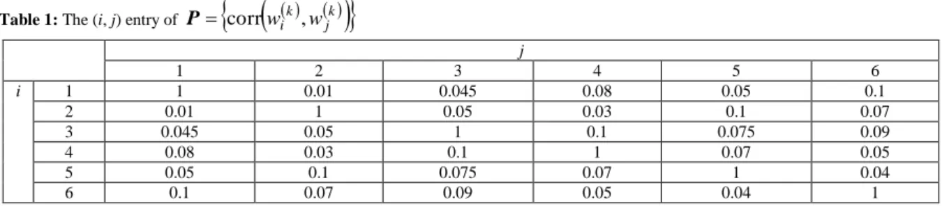
N = 6, T = 10/365, r = 0.05, K = 46.5,a10.2 ,a20.2, a30.2, a40.1, a50.1 and a6 0.2,
k
j k
i w
w ,
corr
P is given in Table 1, i,i,S 0 for i = 1, 2,…, 6, are given in Table 2. The coefficient of
the skewness of vi k (see Eq.(3))
2 3 2 3 3
m m
m with mj E
vi k
j, for j = 2, 3, 4,and the corresponding coefficient of kurtosis
2 2 4 4
m m
m are also given in Table 2.
The results for the American call option prices are shown in Table 3. The computing times required for computing the American call option prices by using the proposed method and simulation (in minutes) respectively in an Intel(R) Core(TM) i5 processor 2.27GHz computer are shown in Table 4.
From Table 3, we can get the following findings:
F1: The American call option prices found by using numerical method agree well with those based on simulation especially when the number ns of points chosen randomly from the N-dimensional space is very
large.
F2: When the distributions of
k i
k i
v deviate from normality (see examples A2, and A3 in Tables 2 and 3), the variation of nv and nr has a rather
large effect on the price based on the numerical method. Thus when the vi k are non-normal, we need to use fairly large nv and nrin order to compute the price accurately.
F3: When the distributions of
k i
v are skewed and having larger kurtosis, the American call option price tends to deviate from the American call option price computed when the distributions of vi k are normal.
From Table 4, we see that the computing times required by the proposed method are comparable to those required by the simulation procedure when ns = 1,000. But when ns = 10,000, the simulation procedure requires
much longer time.
The values of estimated standard error ( , (0 ))
k k
Q t
S x when k = 9, 8, 7 and 6 and m3(i)0 and m4(i)3.0, i = 1, 2, …, 6 are shown in Table 5, while those of ( , (0 ))
k k
Q t
S x for k = 5, 4, 3,…, 1, 0 based on linear extrapolation are shown in Table 6. The last row of Table 6 shows that the standard error of the American option price decreases as we increase the value of nv while keeping nr fixed at 30.
Table 1: The (i, j) entry of
jk
ki w
w ,
corr P
j
1 2 3 4 5 6
i 1 1 0.01 0.045 0.08 0.05 0.1
2 0.01 1 0.05 0.03 0.1 0.07
3 0.045 0.05 1 0.1 0.075 0.09
4 0.08 0.03 0.1 1 0.07 0.05
5 0.05 0.1 0.075 0.07 1 0.04
6 0.1 0.07 0.09 0.05 0.04 1
Table 2: Values of
i,
i, S(0), m3(i) and m4(i)under the three cases A1, A2, and A3Example i
i
i 0
S 3()
i
m m4(i)
A1 1 0.05 0.15 50 0.0 3.0
2 0.05 0.10 60 0.0 3.0
3 0.05 0.20 35 0.0 3.0
4 0.05 0.20 40 0.0 3.0
5 0.05 0.20 45 0.0 3.0
6 0.05 0.20 52 0.0 3.0
A2 1 0.05 0.15 50 0.0 5.0
2 0.05 0.10 60 0.0 5.0
3 0.05 0.20 35 0.0 5.0
4 0.05 0.20 40 0.0 5.0
5 0.05 0.20 45 0.0 5.0
6 0.05 0.20 52 0.0 5.0
A3 1 0.05 0.15 50 0.1 3.6
2 0.05 0.10 60 0.1 3.2
3 0.05 0.20 35 0.1 3.4
4 0.05 0.20 40 0.1 3.0
5 0.05 0.20 45 0.1 3.8
6 0.05 0.20 52 0.1 4.0
Table 3: Results for American call option prices under the three cases A1, A2, and A3
Example (nv, nr) Numerical Method Simulation
ns=1,000 ns=10,000
A1 (50,30) 1.39999 1.40089 1.40059
(100,30) 1.39266 1.40035 1.39412
(200,30) 1.39571 1.40201 1.39725
(300,30) 1.39720 1.40252 1.39788
(400,30) 1.39247 1.40003 1.39275
A2 (50,30) 1.39864 1.40163 1.40048
(100,30) 1.40054 1.41781 1.40443
(200,30) 1.40190 1.41650 1.40259
(300,30) 1.40855 1.41030 1.40828
(400,30) 1.40974 1.41002 1.40996
A3 (50,30) 1.41880 1.41012 1.41677
(100,30) 1.41983 1.41286 1.41530
(200,30) 1.41557 1.41027 1.41546
(300,30) 1.41188 1.41747 1.41054
Table 4: Computation times (in minutes) required for computing the American call option prices presented in Table 3.
(nv, nr) Numerical Method Simulation
ns=1,000 ns=10,000
(50, 30) 120.25 135.21 1650.12
(100, 30) 253.18 270.51 3270.43
(200, 30) 1012.28 1078.36 6510.76
(300,30) 1665.15 1692.67 13030.32
(400,30) 2160.00 2241.39 26040.16
Table 5: The values of estimated standard error ( , (0))
k k
Q t
S x with m3(i) 0 and m4(i)3.0for i = 1, 2, …, 6 when k = 9, 8, 7 and 6
k (nv, nr) = (100, 30) (nv, nr) = (200, 30) (nv, nr) = (300, 30) (nv, nr) = (400, 30)
9 0.00009 0.00005 0.00005 0.00005
8 0.00089 0.00066 0.00054 0.00041
7 0.00199 0.00165 0.00151 0.00145
6 0.00296 0.00246 0.00229 0.00215
Table 6: The estimated values of ( , (0))
k k
Q t
S x obtained by using linear extrapolation.
k (nv, nr) = (100, 30) (nv, nr) = (200, 30) (nv, nr) = (300, 30) (nv, nr) = (400, 30)
5 0.0038 0.0034 0.0029 0.0030
4 0.0048 0.0042 0.0037 0.0037
3 0.0058 0.0050 0.0045 0.0044
2 0.0068 0.0058 0.0053 0.0051
1 0.0078 0.0066 0.0061 0.0058
0 0.0088 0.0074 0.0069 0.0065
Conclusions:
The main contributions of the study include
(A) The introduction of a method based on multivariate quadratic-normal distribution for computing the joint distribution of the vector of time-t asset prices.
(B) The introduction of a method based on regression and numerical integration for pricing multidimensional American options.
(C) The introduction of a method for assessing the accuracy of the computed prices of the American options. The main feature of the methods in this paper is the representation of the N-dimensional function as a quadratic function of the radial distance, with the coefficients of the quadratic function given by second degree polynomials in N-1 polar angles. The above N-dimensional function can approximate fairly well the American option values over the N-dimensional space. Furthermore this representation of the N-dimensional function is attractive from a computational point of view as it leads to easily integrated multiple integrals of which the integrands take the form of a product of N functions of individual variables given by the radial distance and N-1 polar angles.
Although the paper concentrates on the basket call options, it should be interesting to find out whether the methods in the paper may also be adapted to deal with other types of American option, for example the max-option and geometric average max-option.
REFERENCES
Andersen, L., 2000. A Simple Approach to the Pricing of Bermudan Swaptions in the Multi-Factor Libor Market Model. Journal of Computational Finance, 3(1): 5-32.
Avramidis, A.N. and P. Hyden, 1999. Efficiency Improvements for Pricing American Options with a Stochastic Mesh. Proceedings of the 1999 Winter Simulation Conference, pp: 344-350.
Avramidis, A.N. and H. Matzinger, 2004. Convergence of the Stochastic Mesh Estimator for Pricing American Options. Journal of Computational Finance, 7: 73-91.
Barraquand, J. and D. Martineau, 1995. Numerical Valuation of High Dimensional Multivariate American Securities. Journal of Financial and Quantitative Analysis, 30: 383-405.
Beh, W.L., A.H. Pooi and K.L. Goh, 2010. Pricing of American Call Options. Proceedings of the Second International Conference on Computer Research and Development (ICCRD), 2010 IEEE Computer Society Washington, DC, USA, pp: 593-596.
Bossaerts, P., 1989. Simulation Estimators of Optimal Early Exercise. Working paper, Graduate School of Industrial Administration, Carnegie-Mellon University.
Broadie, M. and P. Glasserman, 1997. Pricing American-Style Securities Using Simulation. Journal of Economic Dynamics and Control, 21(8-9): 1323-1352.
Carriére, J., 1996. Valuation of Early-Exercise Price of Options Using Simulations and Non-parametric Regression. Insurance: Mathematics and Economics, 19: 19-30.
Fu, M.C., S.B. Laprise, D.B. Madan, Y. Su and R. Wu, 2001. Pricing American Options: A Comparison of Monte Carlo Simulation Approaches. Journal of Computational Finance, 4: 39-88.
Garcia, D., 2003. Convergence and Biases of Monte Carlo Estimates of American Option Prices Using a Parametric Exercise Rule. Journal of Economic Dynamics and Control, 27: 1855-1879.
Grant, D., G. Vora and D. Weeks, 1997. Path-dependant Options: Extending the Monte Carlo Simulation Approach. Management Science, 43: 1589-1602.
Hunt, K.J., D. Sbarbaro, R. Zbikowski and P.J. Gawthrop, 1992. Neural Networks for Control System – A Survey. Automatica, 28: 1083-1112.
Kelly, D.L., 1994. Valuing and Hedging American Put Options Using Neural Networks. Working paper, Carnegie Mellon University, PA.
Kohler, M. and A. Krzyzak, 2009. Pricing of American Options in Discrete Time Using Least Squares Estimates with Complexity Penalties. Preprint.
Kohler, M., A. Krzyzak and N. Todorovic, 2010. Pricing of High-Dimensional American Options by Neural Networks. Mathematical Finance, 20(3): 383-410.
Li, B. and G. Zhang, 1996. Hurdles Removed. working paper, Merrill Lynch.
Liu, G.W. and L.J. Hong, 2009. Revisit of Stochastic Mesh Method for Pricing American Option. Operations Research Letters, 37: 411-414.
Longstaff, F.A. and E.S. Schwartz, 2001. Valuing American Options by Simulation: A Simple Least-Squares Approach. Review of Financial Studies, 14: 113-147.
Morelli, M.J., G. Montagna, O. Nicrosini, M. Treccani, M. Farina and P. Amato, 2004. Pricing Financial Derivatives with Neural Networks. Physica A: Statistical Mechanics and Its Applications, 338: 160-165.
Pooi, A.H., 2003. Effects of Non-Normality on Confidence Intervals in Linear Models. Technical Report No. 6/2003, Institute of Mathematical Sciences, University of Malaya.
Raymar, S. and M. Zwecher, 1997. Monte Carlo Valuation of American Call Options on Maximum of Several Stocks. Journal of Derivatives, 5: 7-20.
Rogers, L.C.G., 2002. Monte Carlo Valuation of American Options. Mathematical Finance, 12: 271-286. Sanner, R.M. and J.J. Slotine, 1992. Gaussian Networks for Direct Adaptive Control. IEEE Transactions on Neural Networks, 3: 837-863.
Tilley, J.A., 1993. Valuing American Options in Path Simulation Model. Transactions of the Society of Actuaries, 45: 83-104.
Tsitsiklis, J. and B. Van Roy, 1999. Optimal Stopping of Markov Processes: Hilbert Space Theory, Approximation Algorithms, and an Application to Pricing High Dimensional Financial Derivatives. IEEE Transactions on Automatic Control, 44: 1840-1851.