LOCALIZING OBJECTS FAST AND ACCURATELY
Wei Liu
A dissertation submitted to the faculty of the University of North Carolina at Chapel Hill in partial fulfillment of the requirements for the degree of Doctor of Philosophy in
the Department of Computer Science.
Chapel Hill 2016
c 2016 Wei Liu
ABSTRACT
WEI LIU: LOCALIZING OBJECTS FAST AND ACCURATELY. (Under the direction of Alexander C. Berg.)
A fundamental problem in computer vision is knowing what is in the image and where it is. We develop models to localize objects of multiple categories, such as person and car, fast and accurately. In particular, we focus on designing deep convolutional neural networks (CNNs) for object detection and semantic segmentation. A central theme of this dissertation is to explore the design choices of network structure to combine the full power of CNNs and the characteristics of each task to not only achieve high-quality results but also keep the model relatively simple and fast.
At the heart of object detection is the question of how to search efficiently through a continuous 2D bounding boxes space of various scales and aspect ratios at every possible location in an image. A brute force approach would be searching over all possibilities, but it is apparently not scalable and is quite difficult. An alternative is to propose some potential locations which might contain objects, and then classify each of the proposal. Because the search space is much smaller after the proposal step, we can use a more powerful feature to describe each proposal. A first contribution of this dissertation is to show that fine-tuning a much deeper network can boost the detection performance significantly, compared to a relatively shallower network.
A second contribution of this dissertation is that we show that the search can be approximated by discretizing the search space and then regressing the residual difference
between a discrete box and a target box. This is a departure from the proposal and then classify series of methods. We present a single stage framework, SSD, which can simultaneously detect and classify objects fast and accurately. SSD splits the space of small boxes more densely and the space of larger boxes more sparsely. As a result, it can discretize the space more efficiently and ease training notably. We have empirically shown that it is as accurate as or even better than the two-stage methods and yet is much faster.
Unlike object detection, semantic segmentation is usually treated as a per-pixel classi-fication problem, especially in the era of deep networks. However, a major issue is how to incorporate global semantic context information when making local decision. Although there are concurrent works on using techniques from graphical models such as conditional random fields (CRFs) to introduce context and structure information, we present a sim-ple yet effective method, ParseNet, by using the average feature for a layer to augment the features at each location. Experimental results show that it can be as effective as a method which uses CRFs as a post-processing step to include context information.
To my family.
ACKNOWLEDGMENTS
There are so many people I need to thank in my PhD journey, and I am very grateful. I would like to thank my adviser, Alex Berg, from the deepest of my heart. His insight, wisdom and encouragement has always been an inspiration to me. I am very grateful for the freedom and guidance he gave and the trust for letting me organize the ImageNet Large Scale Visual Recognition Challenge (ILSVRC) for two years.
Thanks to my committee members: Tamara Berg, Dragomir Anguelov, Jan-Michael Frahm and Marc Niethammer for giving many suggestions for the final thesis. Thanks to the Berg group: Kota Yamaguchi, Vicente Ordonez, Xufeng Han, Hadi Kiapour, Sirion Vittayakorn, Eunbyung Park, Cheng-Yang Fu, Licheng Yu, Yipin Zhou, Phil Ammi-rato, Patrick Poirson for so many wonderful memories, cheers, discussions, and working together towards many conference deadlines. Thanks to the UNC and Stony Brook Com-puter vision group. Thanks to ILSVRC team: Olga Russakovsky, Jia Deng, Fei-fei Li, and Alex Berg for making ILSVRC 2015-2016 a success.
men-tor, a friend, and a great helper to make single shot detector great and having insightful brainstorming. Thanks to other folks at Google: Yangqing Jia, Pierre Sermanet, Scott Reed, Alex Tosev, George Toderici, Vincent Vanhoucke for helpful discussions. Thanks to Image Understanding and DistBelief team at Google as well.
Thanks to Fernando de la Torre and Alexander Hauptmann for introducing me to computer vision/multimedia research. Thanks to Yuan Shi for being a roommate and encouragement in the first year at CMU. Thanks to Svetlana Lazebnik for her supervision for my first year PhD and initiating the research topic on object detection from video. Thanks to Hongtao Huang for many cheers. Thanks to Lukas Marti for letting me play with computer vision on iPhone. Thanks to the Apple interns that made 2012 summer a great fun and a smooth transition from UNC to Stony Brook. Thanks to so many friends who came across during the journey. Thanks to NVIDIA for donating many GPUs and letting me use their GPU cluster. Thanks to Google Fellowship for supporting my last year of PhD. Thanks to NSF 1452851, 1446631, 1526367, 1533771 for support.
Finally thanks to my parents, Changbai Liu and Shangen Yang, for helping annotate many videos and for everything. Thanks to my wife Yi Zhao for everything always. Thanks to my daughter Angela Liu for giving me tremendous joy everyday. Because of your love and support, I can navigate through the journey and enjoy every moment.
TABLE OF CONTENTS
LIST OF FIGURES . . . xi
LIST OF TABLES . . . .xiii
CHAPTER 1: Introduction . . . .1
1.1 Motivation . . . .1
1.2 Thesis statement . . . .3
1.3 Outline . . . .3
CHAPTER 2: Accurate Object Detection with GoogLeNet . . . .7
2.1 Introduction . . . .7
2.2 Related Work . . . .9
2.3 Region proposal based object detection . . . 11
2.3.1 Region proposals . . . 12
2.3.2 Fine-tuning network. . . 12
2.3.3 Post classification . . . 14
2.3.4 Network architecture . . . 14
2.4 Experiments . . . 18
2.4.1 ILSVRC 2014 Classification Challenge Setup and Results. . . 18
2.4.2 ILSVRC 2014 Detection Challenge Setup and Results . . . 22
CHAPTER 3: Fast Object Detection from Static Images . . . 26
3.1 Introduction . . . 26
3.2 The Single Shot Detector (SSD). . . 28
3.2.1 Model . . . 28
3.2.2 Training . . . 32
3.3 Experimental Results. . . 37
3.3.1 PASCAL VOC2007 . . . 37
3.3.2 Model analysis . . . 39
3.3.3 PASCAL VOC2012 . . . 43
3.3.4 COCO. . . 44
3.3.5 Preliminary ILSVRC results . . . 45
3.3.6 Data Augmentation for Small Object Accuracy . . . 47
3.4 Related Work . . . 53
3.5 Conclusions . . . 55
CHAPTER 4: Fast Semantic Segmentation with Context Cues . . . 57
4.1 Introduction . . . 57
4.2 ParseNet . . . 61
4.2.1 Global Context . . . 61
4.2.2 Early Fusion and Late Fusion . . . 62
4.2.3 L2 Normalization Layer . . . 64
4.3 Experiments . . . 66
4.3.1 Best fine-tuning practices . . . 67
4.3.2 Combining Local and Global Features . . . 69
4.4 Related Work . . . 73
4.5 Conclusion . . . 77
CHAPTER 5: Object Detection from Video . . . 79
5.1 Introduction . . . 79
5.2 Data collection . . . 81
5.2.1 Define the categories . . . 82
5.2.2 Curate the snippets . . . 83
5.2.3 Collect bounding boxes. . . 84
5.2.4 Dataset statistics . . . 85
5.3 Evaluation metric . . . 86
5.3.1 Challenge. . . 86
5.3.2 Main metric . . . 87
5.3.3 Auxiliary metric with tracking . . . 88
5.4 Conclusion and Future Work . . . 91
LIST OF FIGURES
1.1 Introduction to the problems . . . .1
2.1 Region proposal based object detection. . . 13
2.2 Inception module . . . 16
2.3 GoogLeNet network structure . . . 19
2.4 High quality detection examples with GoogLeNet . . . 23
3.1 SSD framework . . . 29
3.2 A comparison between two single shot detection models: SSD and YOLO . . . 30
3.3 Visualization of performance for SSD512 on animals, vehicles, and furniture . . . 40
3.4 Sensitivity and impact of different object characteristics . . . 41
3.5 Detection examples on COCO test-dev with SSD512 model . . . 46
3.6 Sensitivity and impact of object size with new data augmentation . . . 48
3.7 Comparison between SSD300* and SSD512* on coco . . . 50
3.8 Comparison between SSD300* and SSD512* on coco person . . . 51
3.9 Comparison between SSD300* and SSD512* on all coco categories. . . 52
4.1 ParseNet framework . . . 59
4.2 Receptive field (RF) size for last layer . . . 63
4.3 Feature scales for different layers . . . 65
4.4 Global context helps for classifying local patches . . . 74
4.5 Global context confuse local patch predictions . . . 75
5.1 Define video object categories . . . 83
5.2 Curate video snippets . . . 84
5.3 Bounding box annotation GUI . . . 86
5.4 Challenges of object detection from videos . . . 87
5.5 Main metric result in object detection from video over the years . . . 88
LIST OF TABLES
2.1 GoogLeNet incarnation of the Inception architecture . . . 18
2.2 Comparison of classification performance in ILSVRC2014 . . . 21
2.3 Comparison of detection performance in ILSVRC2014 . . . 24
2.4 Comparison of single model detection performance . . . 24
3.1 PASCAL VOC2007 test detection results . . . 38
3.2 Effects of various design choices and components on SSD performance . . . 40
3.3 Effects of using multiple output layers . . . 42
3.4 PASCAL VOC2012 test detection results . . . 44
3.5 COCOtest-dev2015 detection results. . . 45
3.6 Results on multiple datasets by adding image expansion data augmentation . . . 48
3.7 Results on Pascal VOC2007 test . . . 53
4.1 Reproducing FCN-32s on PASCAL-Context . . . 68
4.2 Reproducing DeepLab and DeepLab-LargeFOV results on PASCAL VOC2012 69 4.3 Results on SiftFlow . . . 70
4.4 Results on PASCAL-Context . . . 71
4.5 Adding context for DeepLab-LargeFOV Baseline on VOC2012 . . . 72
4.6 PASCAL VOC2012 test Segmentation results . . . 73
CHAPTER 1: Introduction
What does it mean, to see? The plain man’s answer (and Aristotle’s, too). would be, to know what is where by looking.
– David Marr, Vision
1.1 Motivation
car
stop sign traffic light
person
\
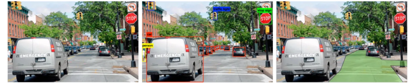
Figure 1.1: This dissertation studies the problem of object detection and semantic
seg-mentation. Object detection is to know the location (e.g. bounding box) of each object;
and semantic segmentation is to know what each pixel is (e.g. drivable path) in an image.
We develop models to localize objects of multiple categories, such as person and car, fast and accurately. In particular, we focus on designing deep convolutional neural networks (CNNs) for object detection and semantic segmentation. A central theme of this dissertation is to explore the design choices of network structure to combine the full power of CNNs and the characteristics of each task to not only achieve high-quality results but also keep the model relatively simple and fast.
At the heart of object detection is the question of how to search efficiently through a continuous 2D bounding boxes space of various scales and aspect ratios at every possible location in an image. A brute force approach would be searching over all possibilities, but it is apparently not scalable and is quite difficult. An alternative is to propose some potential locations which might contain objects, and then classify each of the proposal. Because the search space is much smaller after the proposal step, we can use a more powerful feature to describe each proposal. A first contribution of this dissertation is to show that fine-tuning a much deeper network can boost the detection performance significantly, compared to a relatively shallower network.
A second contribution of this dissertation is that we show that the search can be approximated by discretizing the search space and then regressing the residual difference between a discrete box and a target box. This is a departure from the proposal and then classify series of methods. We present a single stage framework, SSD, which can simultaneously detect and classify objects fast and accurately. SSD splits the space of small boxes more densely and the space of larger boxes more sparsely. As a result, it can discretize the space more efficiently and ease training notably. We have empirically shown that it is as accurate as or even better than the two-stage methods and yet is
much faster.
Unlike object detection, semantic segmentation is usually treated as a per-pixel classi-fication problem, especially in the era of deep networks. However, a major issue is how to incorporate global semantic context information when making local decision. Although there are concurrent works on using techniques from graphical models such as conditional random fields (CRFs) to introduce context and structure information, we present a sim-ple yet effective method, ParseNet, by using the average feature for a layer to augment the features at each location. Experimental results show that it can be as effective as a method which uses CRFs as a post-processing step to include context information.
In order to make the above methods useful for many real-time systems, such as mo-bile devices or self-driving cars, we have collected large-scale video datasets for multiple categories, and hope that temporal consistency information in video can help further boost the performance and speed up the operations while lowering power consumption.
1.2 Thesis statement
Carefully designing and training deep neural networks from large-scale datasets en-ables detecting and segmenting objects of multiple categories fast and accurately.
1.3 Outline
is usually accomplished by modifying the structure of the image-level neural network and fine-tuning it for localization purposes.
Region-based Convolutional Neural Networks (R-CNN) (Girshick et al., 2014) ap-proach object detection as a classification problem over object proposals, followed by regression of the bounding box coordinates. In Chapter 2 we show the process by which we fine-tuned GoogLeNet (Szegedy et al., 2014a) instead of AlexNet (Krizhevsky et al., 2012) using the R-CNN framework and achieved high quality detection results. Addition-ally, we augment the region proposals by combining the Selective Search boxes (Uijlings et al., 2013) with MultiBox predictions (Erhan et al., 2014) for higher recall. Finally, we use an ensemble of 6 GoogLeNet models when classifying each region which improves accuracy from 38.0% to 43.9%, which in turn enabled us to win the ILSVRC2014 DET challenge (Russakovsky et al., 2015) (a world renowned annual event for the visual recog-nition challenge). However, this approach requires classifying thousands of proposals per image, and is therefore very slow.
We are concerned with the efficiency of the model and the simplicity of the training methodology as much as we are about the quality. This not only enables faster turn around for development, but also is particularly useful when deploying the model on real time systems, such as mobile devices or self driving cars, which are sensitive to time delay and usually have limited computational power.
We have demonstrated that by careful design, it is possible to detect objects of mul-tiple categories with a single evaluation of an input image and achieve state-of-the-art performance. In Chapter 3, we present a method for detecting objects in images using a single deep neural network. Our approach, named SSD, discretizes the output space
of bounding boxes into a set of default boxes over different aspect ratios and scales per feature map location. At prediction time, the network generates scores for the pres-ence of each object category in each default box and produces adjustments to the box to better match the object shape. Additionally, the network combines predictions from multiple feature maps with different resolutions to naturally handle objects of various sizes. SSD is simple compared to methods that require object proposals because it com-pletely eliminates proposal generation and subsequent pixel or feature resampling stages and encapsulates all computation in a single network. This makes SSD easy to train and straightforward to integrate into systems that require a detection component. Ex-perimental results on the PASCAL VOC, COCO, and ILSVRC datasets confirm that SSD has competitive accuracy to methods that utilize an additional object proposal step and is much faster, while providing a unified framework for both training and inference. Compared to other single stage methods, SSD has much better accuracy even with a smaller input image size.
is simple, using the average feature for a layer to augment the features at each loca-tion. In addition, we study several idiosyncrasies of training, significantly increasing the performance of baseline FCN network. When we add our proposed global feature, and a technique for learning normalization parameters, accuracy increases consistently even over our improved versions of the baselines. Our proposed approach, ParseNet, achieves state-of-the-art performance on SiftFlow and PASCAL-Context with small additional computational cost over baselines, and near state-of-the-art performance on PASCAL VOC 2012 semantic segmentation with a simple approach.
Our ultimate goal is to develop a system that can localize multiple objects in videos accurately in real time. To achieve this, we have collected a large-scale video dataset across many categories. A naive approach would be applying the techniques we developed from static images to each individual frame of a video, then tracking the most confident detections through time. However, this requires multiple decoupled components (e.g. detector and tracker) and is slow and not optimal. The key problem is how to detect objects accurately per frame and associate objects correctly through time. We believe that combining a recurrent neural network (RNN) and a convolutional neural network (i.e. SSD) can help solve this problem. We leave it for future work.
CHAPTER 2: Accurate Object Detection with GoogLeNet
We need to go deeper.
– Inception
2.1 Introduction
There are many research on how to construct better features (Csurka et al., 2004; Wang et al., 2010; Van De Sande et al., 2010; J´egou et al., 2010; S´anchez et al., 2013) from manually designed local descriptors (Lowe, 2004; Bay et al., 2006; Wang et al., 2009). Selective search (Uijlings et al., 2013) is the first work which shows that the region pro-posal method can outperform the state-of-the-art sliding window method (Felzenszwalb et al., 2008) on PASCAL VOC object detection dataset (Everingham et al., 2010). R-CNN (Girshick et al., 2014) then shows that using the features extracted from a fine-tuned convolutional neural network (i.e. AlexNet (Krizhevsky et al., 2012)) can outperform traditional features by a large margin. The key improvement is that the feature auto-matically learned from a large scale image dataset (Russakovsky et al., 2015) with CNNs is much better than the handcrafted features.
In this work, we show that we can get even better features from a much deeper net-work, which further boost the object detection performance. In specific, we build our accurate object detector using a much deeper and yet efficient neural network architec-ture – GoogLeNet (Szegedy et al., 2014a), and show that it significantly outperforms AlexNet (Krizhevsky et al., 2012) within the similar region proposal based framework. With significantly more layers, the network has much higher capacity to model the com-plexity of visual objects, which enables us to win the ILSVRC 2014 object classification and object detection task1.
1http://image-net.org/challenges/LSVRC/2014/results
2.2 Related Work
Feature matters for almost all visual recognition tasks. There are two mainstream methods for solving object detection: sliding window and region proposal, both of which heavily rely on the power of the feature representation.
Sliding window methods usually requires searching over all possible locations and scales within an image to detect objects, which inevitably forces such methods to use simple features. (Viola and Jones, 2001) used a pool of simple feature detectors, such as rectangle detectors, to quickly reject negative regions in an image by using a boosting classifier. It also applied the cascade idea to further improve the speed of the detector. (Dalal and Triggs, 2005) introduced a simple-to-compute feature, Histogram of Gradient (HoG), and used a linear SVM classifier to detect person in an image. Deformable Part Model (DPM) (Felzenszwalb et al., 2008) extended it further by considering not only whole object but also object parts, and used a latent SVM method to automatically learn to detect both object and object parts and the spatial constraints between them.
method (Felzenszwalb and Huttenlocher, 2004) to make selective search method com-putational feasible on large datasets. Besides, it also proposed the usage of hierarchical segmentation idea to speed up the computational time and maintain the performance. In the most recent works like MultiBox (Erhan et al., 2014; Szegedy et al., 2014b), the se-lective search region proposals, which are based on low-level image features, are replaced by proposals generated directly from a deep neural network.
For object proposal based methods, because there are much less regions to be con-sidered, it is feasible, then, to try more powerful features to help recognize complicated and deformable objects. There are a large number of methods focusing on how to design better feature. Such methods first need to localize distinct regions (Lindeberg, 1998; Mikolajczyk and Schmid, 2004; Matas et al., 2004; Mikolajczyk et al., 2005; Rosten and Drummond, 2006) within an image and extract local image feature descriptors (Lowe, 1999; Berg and Malik, 2001; Belongie et al., 2002; Mikolajczyk and Schmid, 2005; Rublee et al., 2011; Leutenegger et al., 2011; Alahi et al., 2012)), construct visual codebooks by performing k-means clustering (Lloyd, 1982) on these local feature descriptors, and then encode the local features in many different ways (Csurka et al., 2004; Lazebnik et al., 2006; Zhang et al., 2007; Philbin et al., 2008; Van Gemert et al., 2008; Zhou et al., 2010; Wang et al., 2010; Perronnin et al., 2010; J´egou et al., 2010; Chatfield et al., 2011; Van de Sande et al., 2014).
Although powerful, these features are handcrafted and thus are sub-optimal and are not capable of describing the highly complicated visual world. From neuroscience we know that human visual cortex are hierarchical and have multi-stage processes for com-puting features with high level semantic meaning. Neocognitron (Fukushima, 1980) is
an early attempt to mimic such process with hand designed filters. Later (LeCun et al., 1998) used stochastic gradient descent (SGD) via backpropagation (Rumelhart et al., 1985) to train convolutional neural networks (CNNs) to learn the filters as well. The latest widely success of AlexNet on ILSVRC 2012 object classification task (Krizhevsky et al., 2012) has rekindled huge interests in CNNs. (Sharif Razavian et al., 2014) showed that a linear classifier with features extracted from OverFeat (Sermanet et al., 2013), a CNN pretrained on ILSVRC, outperforms all methods which uses traditional handcrafted features on various recognition tasks. Since feature representation of the input image is critical to many recognition tasks, deep network has a huge advantage over traditional computer vision methods because the feature representation learned from large-scale dataset is much better than a handcrafted feature.
The current state-of-the-art for object detection is R-CNN (Girshick et al., 2014), a method uses the object proposal framework. Such a two-stage approach leverages the accuracy of bounding box segmentation with low-level cues, as well as the highly powerful classification power of state-of-the-art CNNs. We adopted a similar pipeline, but have explored enhancements in both stages, such as MultiBox (Erhan et al., 2014) prediction for better region proposals, and ensemble approaches for better categorization of bounding box proposals.
2.3 Region proposal based object detection
dataset, our system needs to fine-tune it on warped proposal windows to adapt it to the object detection dataset. Finally, our system needs to extract a fixed length feature vector from the fine-tuned CNN for each proposal and learn a set of class-specific linear SVMs to post classify each proposal, as shown in Figure 2.1c. In this section, we will describe each steps and the new network architecture in details.
2.3.1 Region proposals
Recently, there are many methods (Carreira and Sminchisescu, 2012; Endres and Hoiem, 2010; Arbelaez et al., 2011; Alexe et al., 2012; Uijlings et al., 2013; Zitnick and Doll´ar, 2014; Arbel´aez et al., 2014) introduced for generating category independent (ag-nostic) region proposals. These methods use different low-level cues of image to generate a large pool of candidate regions of potential objects. In our system, we use the selective search (Uijlings et al., 2013) because it generates the best quality proposals. Besides, we also add about 200 proposals (Erhan et al., 2014) from MultiBox which are learned with a deep network. As a result, we can get very high recall with relatively small number (i.e. 1200) of proposals in each image.
2.3.2 Fine-tuning network
Since we need many data to train a CNN, we have to first use a large-scale dataset to pretrain a model so that it has a good representation of the visual world. Usually we use the ILSVRC classification dataset, which has 1000 classes with 1.2 million training images, to pretrain a model since image level labels are much easier to collect than more detailed annotations such as bounding boxes. Given a network that is first pretrained on
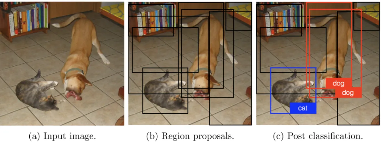
(a) Input image. (b) Region proposals. (c) Post classification.
Figure 2.1: Region proposal based object detection.
object classification datasets, we need to adopt it to the object detection datasets. As opposed to R-CNN (Girshick et al., 2014) which uses AlexNet (Krizhevsky et al., 2012), we use a much deeper and powerful network. We will describe the details of the network architecture later.
Given an object detection dataset where accurate bounding boxes for all objects in an image are provided, we first generate object proposals as described in Sec. 2.3.1. During training time, we treat all proposals with ≥0.5 IoU overlap with a ground truth box as a positive sample for that box’s class and the rest negatives. At each SGD iteration, we sample 32 positive proposals and randomly select 96 negative proposals and crop/warp them to a fixed size (e.g. 227× 227) to form a mini-batch to update the network’s parameters to recognize proposals better.
detection performance.
2.3.3 Post classification
After the fine-tuning, we need to extract features for all proposals within an image. We follow the same procedure as proposed in R-CNN (Girshick et al., 2014). In specific, we crop and warp each proposal region to a fixed image size (e.g. 227×227). Then we forward the warped proposal to the fine-tuned network to extract the final feature layer (before the 1000-way classification layer) and save it as the feature representation for each proposal. Then we train a binary linear SVM classifier for each object category independently using the extracted features. We use the ground truth boxes as positive samples and use hard negative mining methods (Felzenszwalb et al., 2008) to select hard negative samples during training.
2.3.4 Network architecture
The major contribution of this work is that we use a much deeper and powerful network, which results in better feature and improve the object detection performance significantly. We now describe the motivation and details of the network.
The most straightforward way of improving the performance of deep neural networks is by increasing their size. This includes both increasing the depth – the number of network levels – as well as its width: the number of units at each level. This is an easy and safe way of training higher quality models, especially given the availability of a large amount of labeled training data. However, this simple solution comes with two major drawbacks.
Bigger size typically means a larger number of parameters, which makes the enlarged network more prone to over-fitting. The other drawback of uniformly increased network size is the dramatically increased use of computational resources. For example, in a deep vision network, if two convolutional layers are chained, any uniform increase in the number of their filters results in a quadratic increase of computation.
Inception module
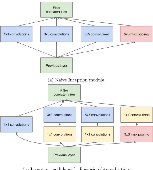
A fundamental way of solving both of these issues would be to introduce sparsity and replace the fully connected layers by the sparse ones, even inside the convolutions. The well known Hebbian principle – neurons that fire together, wire together – suggests that we could use convolution kernels to learn to associate similar patterns. Besides, consid-ering the natural of multiple scales of objects, we apply convolutional kernel of multiple sizes (e.g. 1, 3×3, and 5×5) on an input layer and concatenate the resulted feature maps, which becomes the input of the next stage. Additionally, since pooling operations have been essential for the success of current convolutional networks, it suggests that adding an alternative parallel pooling path in each such stage should have additional beneficial effect, too. Figure 2.2a shows an naive Inception module which embodies the idea.
1x1 convolutions 3x3 convolutions 5x5 convolutions Filter
concatenation
Previous layer
3x3 max pooling
(a) Inception module, na¨ıve version
1x1 convolutions
3x3 convolutions 5x5 convolutions Filter
concatenation
Previous layer
3x3 max pooling 1x1 convolutions 1x1 convolutions
1x1 convolutions
(b) Inception module with dimensionality reduction
Figure 2: Inception module
ber of filters in the previous stage. The merging of output
of the pooling layer with outputs of the convolutional
lay-ers would lead to an inevitable increase in the number of
outputs from stage to stage. While this architecture might
cover the optimal sparse structure, it would do it very
inef-ficiently, leading to a computational blow up within a few
stages.
This leads to the second idea of the Inception
architec-ture: judiciously reducing dimension wherever the
compu-tational requirements would increase too much otherwise.
This is based on the success of embeddings: even low
di-mensional embeddings might contain a lot of information
about a relatively large image patch. However,
embed-dings represent information in a dense, compressed form
and compressed information is harder to process. The
rep-resentation should be kept sparse at most places (as required
by the conditions of [2]) and compress the signals only
whenever they have to be aggregated en masse. That is,
1
⇥
1
convolutions are used to compute reductions before
the expensive
3
⇥
3
and
5
⇥
5
convolutions. Besides being
used as reductions, they also include the use of rectified
lin-ear activation making them dual-purpose. The final result is
depicted in Figure 2(b).
In general, an Inception network is a network
consist-ing of modules of the above type stacked upon each other,
with occasional max-pooling layers with stride 2 to halve
the resolution of the grid. For technical reasons (memory
efficiency during training), it seemed beneficial to start
us-ing Inception modules only at higher layers while keepus-ing
the lower layers in traditional convolutional fashion. This is
not strictly necessary, simply reflecting some infrastructural
inefficiencies in our current implementation.
A useful aspect of this architecture is that it allows for
increasing the number of units at each stage significantly
without an uncontrolled blow-up in computational
com-plexity at later stages. This is achieved by the ubiquitous
use of dimensionality reduction prior to expensive
convolu-tions with larger patch sizes. Furthermore, the design
fol-lows the practical intuition that visual information should
be processed at various scales and then aggregated so that
the next stage can abstract features from the different scales
simultaneously.
The improved use of computational resources allows for
increasing both the width of each stage as well as the
num-ber of stages without getting into computational difficulties.
One can utilize the Inception architecture to create slightly
inferior, but computationally cheaper versions of it. We
have found that all the available knobs and levers allow for
a controlled balancing of computational resources resulting
in networks that are
3
10
⇥
faster than similarly
perform-ing networks with non-Inception architecture, however this
requires careful manual design at this point.
5. GoogLeNet
By the“GoogLeNet” name we refer to the particular
in-carnation of the Inception architecture used in our
submis-sion for the ILSVRC 2014 competition. We also used one
deeper and wider Inception network with slightly superior
quality, but adding it to the ensemble seemed to improve the
results only marginally. We omit the details of that network,
as empirical evidence suggests that the influence of the
ex-act architectural parameters is relatively minor. Table 1
il-lustrates the most common instance of Inception used in the
competition. This network (trained with different
image-patch sampling methods) was used for 6 out of the 7 models
in our ensemble.
All the convolutions, including those inside the
Incep-tion modules, use rectified linear activaIncep-tion. The size of the
receptive field in our network is
224
⇥
224
in the RGB color
space with zero mean. “
#3
⇥
3
reduce” and “
#5
⇥
5
reduce”
stands for the number of
1
⇥
1
filters in the reduction layer
used before the
3
⇥
3
and
5
⇥
5
convolutions. One can see
the number of
1
⇥
1
filters in the projection layer after the
built-in max-pooling in the pool proj column. All these
re-duction/projection layers use rectified linear activation as
well.
The network was designed with computational efficiency
and practicality in mind, so that inference can be run on
in-dividual devices including even those with limited
compu-tational resources, especially with low-memory footprint.
(a) Naive Inception module.
1x1 convolutions 3x3 convolutions 5x5 convolutions
Filter concatenation
Previous layer
3x3 max pooling
(a) Inception module, na¨ıve version
1x1 convolutions
3x3 convolutions 5x5 convolutions
Filter concatenation
Previous layer
3x3 max pooling
1x1 convolutions 1x1 convolutions
1x1 convolutions
(b) Inception module with dimensionality reduction
Figure 2: Inception module
ber of filters in the previous stage. The merging of output
of the pooling layer with outputs of the convolutional
lay-ers would lead to an inevitable increase in the number of
outputs from stage to stage. While this architecture might
cover the optimal sparse structure, it would do it very
inef-ficiently, leading to a computational blow up within a few
stages.
This leads to the second idea of the Inception
architec-ture: judiciously reducing dimension wherever the
compu-tational requirements would increase too much otherwise.
This is based on the success of embeddings: even low
di-mensional embeddings might contain a lot of information
about a relatively large image patch. However,
embed-dings represent information in a dense, compressed form
and compressed information is harder to process. The
rep-resentation should be kept sparse at most places (as required
by the conditions of [2]) and compress the signals only
whenever they have to be aggregated en masse. That is,
1
⇥
1
convolutions are used to compute reductions before
the expensive
3
⇥
3
and
5
⇥
5
convolutions. Besides being
used as reductions, they also include the use of rectified
lin-ear activation making them dual-purpose. The final result is
depicted in Figure 2(b).
In general, an Inception network is a network
consist-ing of modules of the above type stacked upon each other,
with occasional max-pooling layers with stride 2 to halve
the resolution of the grid. For technical reasons (memory
efficiency during training), it seemed beneficial to start
us-ing Inception modules only at higher layers while keepus-ing
the lower layers in traditional convolutional fashion. This is
not strictly necessary, simply reflecting some infrastructural
inefficiencies in our current implementation.
A useful aspect of this architecture is that it allows for
increasing the number of units at each stage significantly
without an uncontrolled blow-up in computational
com-plexity at later stages. This is achieved by the ubiquitous
use of dimensionality reduction prior to expensive
convolu-tions with larger patch sizes. Furthermore, the design
fol-lows the practical intuition that visual information should
be processed at various scales and then aggregated so that
the next stage can abstract features from the different scales
simultaneously.
The improved use of computational resources allows for
increasing both the width of each stage as well as the
num-ber of stages without getting into computational difficulties.
One can utilize the Inception architecture to create slightly
inferior, but computationally cheaper versions of it. We
have found that all the available knobs and levers allow for
a controlled balancing of computational resources resulting
in networks that are
3
10
⇥
faster than similarly
perform-ing networks with non-Inception architecture, however this
requires careful manual design at this point.
5. GoogLeNet
By the“GoogLeNet” name we refer to the particular
in-carnation of the Inception architecture used in our
submis-sion for the ILSVRC 2014 competition. We also used one
deeper and wider Inception network with slightly superior
quality, but adding it to the ensemble seemed to improve the
results only marginally. We omit the details of that network,
as empirical evidence suggests that the influence of the
ex-act architectural parameters is relatively minor. Table 1
il-lustrates the most common instance of Inception used in the
competition. This network (trained with different
image-patch sampling methods) was used for 6 out of the 7 models
in our ensemble.
All the convolutions, including those inside the
Incep-tion modules, use rectified linear activaIncep-tion. The size of the
receptive field in our network is
224
⇥
224
in the RGB color
space with zero mean. “
#3
⇥
3
reduce” and “
#5
⇥
5
reduce”
stands for the number of
1
⇥
1
filters in the reduction layer
used before the
3
⇥
3
and
5
⇥
5
convolutions. One can see
the number of
1
⇥
1
filters in the projection layer after the
built-in max-pooling in the pool proj column. All these
re-duction/projection layers use rectified linear activation as
well.
The network was designed with computational efficiency
and practicality in mind, so that inference can be run on
in-dividual devices including even those with limited
compu-tational resources, especially with low-memory footprint.
(b) Inception module with dimensionality reduction.
Figure 2.2: Inception module.
outputs of the convolutional layers would lead to an inevitable increase in the number of outputs from stage to stage, leading to a computational blow up within a few stages.
This leads to the second idea of the Inception architecture: judiciously reducing dimension wherever the computational requirements would increase too much otherwise. In specific, 1×1 convolutions are used to compute reductions before the expensive 3×3 and 5 ×5 convolutions. The final result is depicted in Figure 2.2b. This allows for increasing both the width of each stage as well as the number of stages without getting into computational difficulties.
GoogLeNet
In general, an Inception network is a network consisting of modules of the above type stacked upon each other, with occasional max-pooling layers with stride 2 to halve the resolution of the grid. By the ”GoogLeNet” name we refer to the particular incarnation of the Inception architecture used in our submission for the ILSVRC 2014 competition.
Table 2.1 illustrates the most common instance of Inception used in the competition. All the convolutions, including those inside the Inception modules, use rectified linear activation (Nair and Hinton, 2010). The size of the receptive field in our network is 224×224 in the RGB color space with zero mean. ”#3×3 reduce” and ”#5×5 reduce” stands for the number of 1×1 filters in the reduction layer used before the 3×3 and 5×5 convolutions. One can see the number of 1×1 filters in the projection layer after the built-in max-pooling in the ”pool proj” column. All these reduction/projection layers use rectified linear activation as well.
type patch size/stride outputsize depth #1⇥1 #3⇥3
reduce #3⇥3 reduce#5⇥5 #5⇥5 poolproj params ops
convolution 7⇥7/2 112⇥112⇥64 1 2.7K 34M
max pool 3⇥3/2 56⇥56⇥64 0
convolution 3⇥3/1 56⇥56⇥192 2 64 192 112K 360M
max pool 3⇥3/2 28⇥28⇥192 0
inception (3a) 28⇥28⇥256 2 64 96 128 16 32 32 159K 128M
inception (3b) 28⇥28⇥480 2 128 128 192 32 96 64 380K 304M
max pool 3⇥3/2 14⇥14⇥480 0
inception (4a) 14⇥14⇥512 2 192 96 208 16 48 64 364K 73M
inception (4b) 14⇥14⇥512 2 160 112 224 24 64 64 437K 88M
inception (4c) 14⇥14⇥512 2 128 128 256 24 64 64 463K 100M
inception (4d) 14⇥14⇥528 2 112 144 288 32 64 64 580K 119M
inception (4e) 14⇥14⇥832 2 256 160 320 32 128 128 840K 170M
max pool 3⇥3/2 7⇥7⇥832 0
inception (5a) 7⇥7⇥832 2 256 160 320 32 128 128 1072K 54M
inception (5b) 7⇥7⇥1024 2 384 192 384 48 128 128 1388K 71M
avg pool 7⇥7/1 1⇥1⇥1024 0
dropout (40%) 1⇥1⇥1024 0
linear 1⇥1⇥1000 1 1000K 1M
softmax 1⇥1⇥1000 0
Table 1: GoogLeNet incarnation of the Inception architecture.
The network is 22 layers deep when counting only layers with parameters (or 27 layers if we also count pooling). The overall number of layers (independent building blocks) used for the construction of the network is about 100. The exact number depends on how layers are counted by the machine learning infrastructure. The use of average pooling before the classifier is based on [12], although our implementation has an additional linear layer. The linear layer enables us to easily adapt our networks to other label sets, however it is used mostly for convenience and we do not expect it to have a major effect. We found that a move from fully connected layers to average pooling improved the top-1 accuracy by about 0.6%, however the use of dropout remained essential even after removing the fully connected layers.
Given relatively large depth of the network, the ability to propagate gradients back through all the layers in an effective manner was a concern. The strong performance of shallower networks on this task suggests that the fea-tures produced by the layers in the middle of the network should be very discriminative. By adding auxiliary classi-fiers connected to these intermediate layers, discrimination in the lower stages in the classifier was expected. This was thought to combat the vanishing gradient problem while
providing regularization. These classifiers take the form of smaller convolutional networks put on top of the out-put of the Inception (4a) and (4d) modules. During train-ing, their loss gets added to the total loss of the network with a discount weight (the losses of the auxiliary classi-fiers were weighted by 0.3). At inference time, these auxil-iary networks are discarded. Later control experiments have shown that the effect of the auxiliary networks is relatively minor (around 0.5%) and that it required only one of them to achieve the same effect.
The exact structure of the extra network on the side, in-cluding the auxiliary classifier, is as follows:
• An average pooling layer with 5⇥5 filter size and
stride3, resulting in an4⇥4⇥512output for the (4a),
and4⇥4⇥528for the (4d) stage.
• A1⇥1convolution with 128 filters for dimension
re-duction and rectified linear activation.
• A fully connected layer with 1024 units and rectified linear activation.
• A dropout layer with 70% ratio of dropped outputs.
Table 2.1: GoogLeNet incarnation of the Inception architecture.
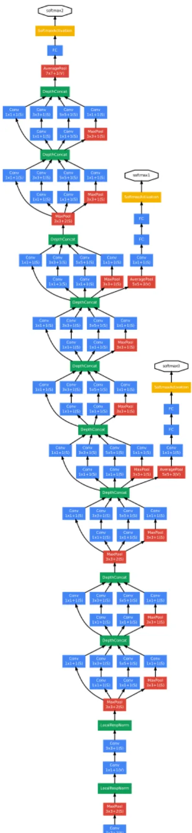
that inference can be run on individual devices including even those with limited compu-tational resources, especially with low-memory footprint. Figure 2.3 shows the resulting network architecture. For more details, please refer to the original paper (Szegedy et al., 2014a).
2.4 Experiments
2.4.1 ILSVRC 2014 Classification Challenge Setup and Results
The ILSVRC 2014 classification challenge involves the task of classifying the image into one of 1000 leaf-node categories in the ImageNet hierarchy. There are about 1.2 million images for training, 50,000 for validation and 100,000 images for testing. Each image is associated with one ground truth category, and performance is measured based
• A linear layer with softmax loss as the classifier (pre-dicting the same 1000 classes as the main classifier, but removed at inference time).
A schematic view of the resulting network is depicted in Figure 3.
6. Training Methodology
GoogLeNet networks were trained using the DistBe-lief [4] distributed machine learning system using mod-est amount of model and data-parallelism. Although we used a CPU based implementation only, a rough estimate suggests that the GoogLeNet network could be trained to convergence using few high-end GPUs within a week, the main limitation being the memory usage. Our training used asynchronous stochastic gradient descent with 0.9 momen-tum [17], fixed learning rate schedule (decreasing the learn-ing rate by 4% every 8 epochs). Polyak averaglearn-ing [13] was used to create the final model used at inference time.
Image sampling methods have changed substantially over the months leading to the competition, and already converged models were trained on with other options, some-times in conjunction with changed hyperparameters, such as dropout and the learning rate. Therefore, it is hard to give a definitive guidance to the most effective single way to train these networks. To complicate matters further, some of the models were mainly trained on smaller relative crops, others on larger ones, inspired by [8]. Still, one prescrip-tion that was verified to work very well after the competi-tion, includes sampling of various sized patches of the im-age whose size is distributed evenly between 8% and 100% of the image area with aspect ratio constrained to the inter-val[34,43]. Also, we found that the photometric distortions of Andrew Howard [8] were useful to combat overfitting to the imaging conditions of training data.
7. ILSVRC 2014 Classification Challenge Setup and Results
The ILSVRC 2014 classification challenge involves the task of classifying the image into one of 1000 leaf-node cat-egories in the Imagenet hierarchy. There are about 1.2 mil-lion images for training, 50,000 for validation and 100,000 images for testing. Each image is associated with one ground truth category, and performance is measured based on the highest scoring classifier predictions. Two num-bers are usually reported: the top-1 accuracy rate, which compares the ground truth against the first predicted class, and the top-5 error rate, which compares the ground truth against the first 5 predicted classes: an image is deemed correctly classified if the ground truth is among the top-5, regardless of its rank in them. The challenge uses the top-5 error rate for ranking purposes.
input Conv 7x7+2(S) MaxPool 3x3+2(S) LocalRespNorm Conv 1x1+1(V) Conv 3x3+1(S) LocalRespNorm MaxPool 3x3+2(S) Conv 1x1+1(S) Conv
1x1+1(S) 1x1+1(S)Conv 3x3+1(S)MaxPool DepthConcat Conv
3x3+1(S) 5x5+1(S)Conv 1x1+1(S)Conv Conv
1x1+1(S) Conv
1x1+1(S) 1x1+1(S)Conv 3x3+1(S)MaxPool DepthConcat Conv
3x3+1(S) 5x5+1(S)Conv 1x1+1(S)Conv MaxPool 3x3+2(S) Conv 1x1+1(S)
Conv
1x1+1(S) 1x1+1(S)Conv 3x3+1(S)MaxPool DepthConcat Conv
3x3+1(S) 5x5+1(S)Conv 1x1+1(S)Conv Conv
1x1+1(S) Conv
1x1+1(S) 1x1+1(S)Conv 3x3+1(S)MaxPool AveragePool5x5+3(V) DepthConcat
Conv
3x3+1(S) 5x5+1(S)Conv 1x1+1(S)Conv Conv
1x1+1(S) Conv
1x1+1(S) 1x1+1(S)Conv 3x3+1(S)MaxPool DepthConcat Conv 3x3+1(S) Conv 5x5+1(S) Conv 1x1+1(S) Conv 1x1+1(S) Conv
1x1+1(S) 1x1+1(S)Conv 3x3+1(S)MaxPool DepthConcat Conv
3x3+1(S) 5x5+1(S)Conv 1x1+1(S)Conv Conv
1x1+1(S) Conv
1x1+1(S) 1x1+1(S)Conv 3x3+1(S)MaxPool AveragePool5x5+3(V) DepthConcat
Conv
3x3+1(S) 5x5+1(S)Conv 1x1+1(S)Conv MaxPool
3x3+2(S) Conv
1x1+1(S) Conv
1x1+1(S) 1x1+1(S)Conv 3x3+1(S)MaxPool DepthConcat Conv
3x3+1(S) 5x5+1(S)Conv 1x1+1(S)Conv Conv
1x1+1(S) Conv
1x1+1(S) 1x1+1(S)Conv 3x3+1(S)MaxPool DepthConcat Conv
3x3+1(S) 5x5+1(S)Conv 1x1+1(S)Conv AveragePool 7x7+1(V) FC Conv 1x1+1(S) FC FC SoftmaxActivation softmax0 Conv 1x1+1(S) FC FC SoftmaxActivation softmax1 SoftmaxActivation softmax2
Figure 3: GoogLeNet network with all the bells and whistles.
on the highest scoring classifier predictions. Two numbers are usually reported: the top-1 accuracy rate, which compares the ground truth against the first predicted class, and the top-5 error rate, which compares the ground truth against the first 5 predicted classes: an image is deemed correctly classified if the ground truth is among the top-5, regardless of its rank in them. The challenge uses the top-5 error rate for ranking purposes.
We participated in the challenge with no external data used for training. We adopted a set of techniques during testing to obtain a higher performance, which we describe next.
• We independently trained 7 versions of the same GoogLeNet model (including one wider version), and performed ensemble prediction with them. These models were trained with the same initialization (even with the same initial weights, due to an oversight) and learning rate policies. They differed only in sampling methodologies and the randomized input image order.
• During testing, we adopted a more aggressive cropping approach than that of AlexNet (Krizhevsky et al., 2012). Specifically, we resized the image to 4 scales where the shorter dimension (height or width) is 256, 288, 320 and 352 respec-tively, take the left, center and right square of these resized images (in the case of portrait images, we take the top, center and bottom squares). For each square, we then take the 4 corners and the center 224×224 crop as well as the square resized to 224×224, and their mirrored versions. This leads to 4×3×6×2 = 144 crops per image. A similar approach was used by Andrew Howard (Howard, 2013) in the previous year’s entry, which we empirically verified to perform slightly worse
than the proposed scheme. We note that such aggressive cropping may not be necessary in real applications, as the benefit of more crops becomes marginal after a reasonable number of crops are present (as we will show later on).
• The softmax probabilities are averaged over multiple crops and over all the indi-vidual classifiers to obtain the final prediction. In our experiments we analyzed alternative approaches on the validation data, such as max pooling over crops and averaging over classifiers, but they lead to inferior performance than the simple averaging.
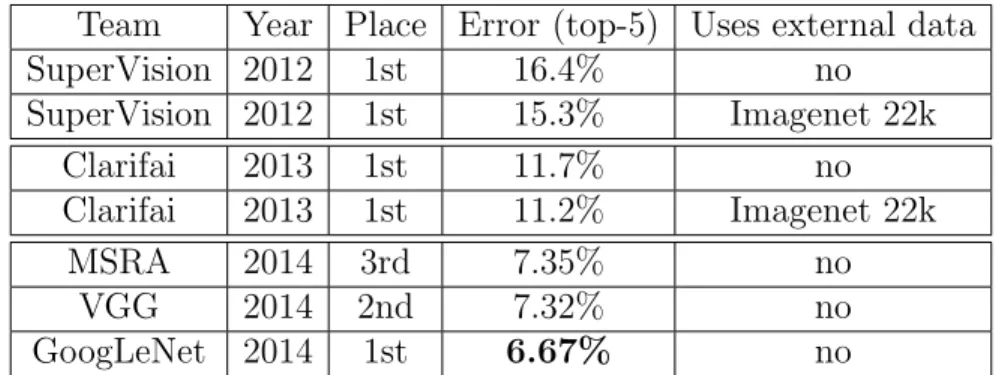
Our final submission to the challenge obtains a top-5 error of 6.67% on both the validation and testing data, ranking the first among other participants. This is a 56.5% relative reduction compared to the SuperVision approach in 2012, and about 40% relative reduction compared to the previous year’s best approach (Clarifai) (Zeiler and Fergus, 2014), both of which used external data for training the classifiers. Table 2.2 shows the statistics of some of the top-performing approaches over the past 3 years.
Team Year Place Error (top-5) Uses external data
SuperVision 2012 1st 16.4% no
SuperVision 2012 1st 15.3% Imagenet 22k
Clarifai 2013 1st 11.7% no
Clarifai 2013 1st 11.2% Imagenet 22k
MSRA 2014 3rd 7.35% no
VGG 2014 2nd 7.32% no
GoogLeNet 2014 1st 6.67% no
2.4.2 ILSVRC 2014 Detection Challenge Setup and Results
ILSVRC uses mean Average Precision (mAP) to measure the accuracy of object detection methods. A method produces arbitrary number of detection results for each object classes in each image. Each detection result has the format of (bij, sij) for image
Ii and object classCj, where bij is the bounding box and sij is the score. The detection
results are first sorted in descending order based on detection scores, and are then greedily matched to the ground truth boxes. A detection result is considered as a true positive if the intersection over union (IoU) overlap with a ground truth box is more than 50%; otherwise it is considered as a false positive.
Note that it also penalizes duplicate detections. In other words, if there are multiple detections for an object (e.g. IoU threshold>0.5), only the detection with highest score is a true positive and all others are false positives. Given this information, we can then compute precision as the fraction correct detections among all the detections reported, and recall as the fraction of detected ground truth objects, for each object class. We then compute average precision (AP) as the area under the precision/recall curve for each object class, and mAP as the average from all object classes.
The approach we take is similar to R-CNN by (Girshick et al., 2014), which first generates object proposals and then post-classify each proposal using deep convolutional network. Instead of using AlexNet (Krizhevsky et al., 2012) as the post-classifier, we replace it with the GoogLeNet (Szegedy et al., 2014a) which has many more layers and thus much larger capacity. Additionally, we augment the region proposals by combining the selective search boxes (Uijlings et al., 2013) with MultiBox predictions (Erhan et al.,
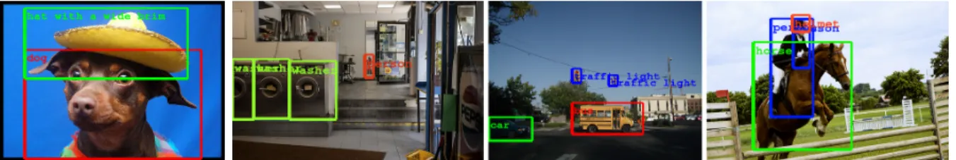
2014) for higher recall. In specific, we increase the proposal size by 2×, which halves the number of selective search object proposals. Besides, we add 200 region proposals generated by MultiBox (Erhan et al., 2014). As a result, we use about 60% of the proposals used in (Girshick et al., 2014), and increase the recall from 92% to 93%, which improve the mean average precision by 1% for a single model. Finally, we use an ensemble of 6 GoogLeNet models when classifying each region which improves accuracy from 38.0% to 43.9%. Note that we did not use bounding box regression as used in R-CNN. Figure 2.4 shows some high quality detection examples returned by the system.
Figure 2.4: High quality detection examples. We ranked 1st in the ILSVRC2014 DET track (Russakovsky et al., 2015).
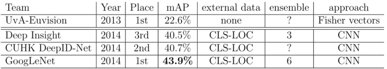
Team Year Place mAP external data ensemble approach
UvA-Euvision 2013 1st 22.6% none ? Fisher vectors
Deep Insight 2014 3rd 40.5% CLS-LOC 3 CNN
CUHK DeepID-Net 2014 2nd 40.7% CLS-LOC ? CNN
GoogLeNet 2014 1st 43.9% CLS-LOC 6 CNN
Table 2.3: Results on ILSVRC2014 object detection external track. Unreported values are noted with question marks.
In Table 2.4, we compare results using a single model only. All the methods fol-lowed the R-CNN framework (Girshick et al., 2014) with slightly different region pro-posals and different CNN models. Notably DeepID-Net proposed a new deformation layer which learns the deformable between object parts and the whole object as was done in DPM (Felzenszwalb et al., 2008), and was built on ZFNet (Zeiler and Fergus, 2014) – a network with same depth and accuracy as AlexNet. Our single model has similar accuracy even without this extra information because of the extraordinary power of GoogLeNet. The top performing model is by Deep Insight, which used context and bounding box regression as extra steps for their detector. Surprisingly it only improves by 0.3 points with an ensemble of 3 models while the GoogLeNet obtains significantly stronger results with the ensemble.
Team mAP Contextual model Bounding box regression
Trimps-Soushen 31.6% no ?
Berkeley Vision 34.5% no yes
UvA-Euvision 35.4% ? ?
CUHK DeepID-Net 37.7% no ?
GoogLeNet 38.0% no no
Deep Insight 40.2% yes yes
Table 2.4: Single model performance for ILSVRC2014 object detection exter-nal track.
2.5 Conclusion
CHAPTER 3: Fast Object Detection from Static Images
Everything should be made as simple as possible, but not simpler.
– Albert Einstein
3.1 Introduction
Current state-of-the-art object detection systems are variants of the following proach: hypothesize bounding boxes, resample pixels or features for each box, and ap-ply a high-quality classifier. This pipeline has prevailed on detection benchmarks since the Selective Search work (Uijlings et al., 2013) through the current leading results on PASCAL VOC, COCO, and ILSVRC detection all based on Faster R-CNN(Ren et al., 2015) albeit with deeper features such as (He et al., 2016). While accurate, these ap-proaches have been too computationally intensive for embedded systems and, even with high-end hardware, too slow for real-time applications. Often detection speed for these approaches is measured in seconds per frame (SPF), and even the fastest high-accuracy detector, Faster R-CNN, operates at only 7 frames per second (FPS). There have been many attempts to build faster detectors by attacking each stage of the detection pipeline (see related work in Sec. 4.4), but so far, significantly increased speed comes only at the cost of significantly decreased detection accuracy.
do. This results in a significant improvement in speed for high-accuracy detection (59 FPS with mAP 74.3% on VOC2007 test, vs. Faster R-CNN 7 FPS with mAP 73.2% or YOLO 45 FPS with mAP 63.4%). The fundamental improvement in speed comes from eliminating bounding box proposals and the subsequent pixel or feature resampling stage. We are not the first to do this (cf (Sermanet et al., 2013; Redmon et al., 2015)), but by adding a series of improvements, we manage to increase the accuracy significantly over previous attempts. Our improvements include using a small convolutional filter to predict object categories and offsets in bounding box locations, using separate predictors (filters) for different aspect ratio detections, and applying these filters to multiple fea-ture maps from the later stages of a network in order to perform detection at multiple scales. With these modifications—especially using multiple layers for prediction at dif-ferent scales—we can achieve high-accuracy using relatively low resolution input, further increasing detection speed. While these contributions may seem small independently, we note that the resulting system improves accuracy on real-time detection for PASCAL VOC from 63.4% mAP for YOLO to 74.3% mAP for our SSD. This is a larger relative improvement in detection accuracy than that from the recent, very high-profile work on residual networks (He et al., 2016). Furthermore, significantly improving the speed of high-quality detection can broaden the range of settings where computer vision is useful.
We summarize our contributions as follows:
proposals and pooling (including Faster R-CNN).
• The core of SSD is predicting category scores and box offsets for a fixed set of default bounding boxes using small convolutional filters applied to feature maps.
• To achieve high detection accuracy we produce predictions of different scales from feature maps of different scales, and explicitly separate predictions by aspect ratio.
• These design features lead to simple end-to-end training and high accuracy, even on low resolution input images, further improving the speed vs accuracy trade-off.
• Experiments include timing and accuracy analysis on models with varying input size evaluated on PASCAL VOC, COCO, and ILSVRC and are compared to a range of recent state-of-the-art approaches.
3.2 The Single Shot Detector (SSD)
This section describes our proposed SSD framework for detection (Sec. 3.2.1) and the associated training methodology (Sec. 3.2.2). Afterwards, Sec. 3.3 presents dataset-specific model details and experimental results.
3.2.1 Model
The SSD approach is based on a feed-forward convolutional network that produces a fixed-size collection of bounding boxes and scores for the presence of object class in-stances in those boxes, followed by a non-maximum suppression step to produce the final detections. The early network layers are based on a standard architecture used for high
(a) Image with GT boxes
(b) 8
×
8 feature map (c) 4
×
4 feature map
loc
:
∆(
cx, cy, w, h
)
conf
:
(
c
1, c
2,
· · ·
, c
p)
Figure 3.1: SSD framework. (a) SSD only needs an input image and ground truth boxes for each object during training. In a convolutional fashion, we evaluate a small set (e.g. 4) of default boxes of different aspect ratios at each location in several feature maps with different scales (e.g. 8×8 and 4×4 in (b) and (c)). For each default box, we predict both the shape offsets and the confidences for all object categories ((c1, c2,· · · , cp)). At
training time, we first match these default boxes to the ground truth boxes. For example, we have matched two default boxes with the cat and one with the dog, which are treated as positives and the rest as negatives. The model loss is a weighted sum between localization loss (e.g. Smooth L1 (Girshick, 2015)) and confidence loss (e.g. Softmax).
quality image classification (truncated before any classification layers), which we will call the base network1. We then add auxiliary structure to the network to produce detections with the following key features:
Multi-scale feature maps for detection
We add convolutional feature layers to the end of the truncated base network. These layers decrease in size progressively and allow predictions of detections at multiple scales. The convolutional model for predicting detections is different for each feature layer (cf
Overfeat(Sermanet et al., 2013) and YOLO(Redmon et al., 2015) that operate on a single scale feature map).
300 300
3
VGG-16
through Conv5_3 layer
19 19 Conv7 (FC7) 1024 10 10 Conv8_2 512 5 5 Conv9_2 256 3 Conv10_2 256 256 38 38 Conv4_3 3 1 Image
Conv: 1x1x1024 Conv: 1x1x256 Conv: 3x3x512-s2
Conv: 1x1x128 Conv: 3x3x256-s2
Conv: 1x1x128 Conv: 3x3x256-s1
Detections:8732 per Class
Classifier : Conv: 3x3x(4x(Classes+4))
512 448 448 3 Image 7 7 1024 7 7 30 Fully Connected
YOLO Customized Architecture
Non-Maximum Suppression
Fully Connected
Non-Maximum Suppression
Detections: 98 per class
Conv11_2
74.3mAP 59FPS
63.4mAP 45FPS
Classifier : Conv: 3x3x(6x(Classes+4))
19 19 Conv6 (FC6) 1024 Conv: 3x3x1024 SSD YOLO
Extra Feature Layers
Conv: 1x1x128 Conv: 3x3x256-s1 Conv: 3x3x(4x(Classes+4))
Figure 3.2: A comparison between two single shot detection models: SSD and YOLO(Redmon et al., 2015). Our SSD model adds several feature layers to the end of a base network, which predict the offsets to default boxes of different scales and aspect ratios and their associated confidences. SSD with a 300×300 input size significantly outperforms its 448×448 YOLO counterpart in accuracy on VOC2007 test while also improving the speed.
Convolutional predictors for detection
Each added feature layer (or optionally an existing feature layer from the base net-work) can produce a fixed set of detection predictions using a set of convolutional filters. These are indicated on top of the SSD network architecture in Fig. 3.2. For a feature layer of size m×n with p channels, the basic element for predicting parameters of a potential detection is a 3×3×psmall kernel that produces either a score for a category, or a shape offset relative to the default box coordinates. At each of the m×n locations where the kernel is applied, it produces an output value. The bounding box offset out-put values are measured relative to a default box position relative to each feature map location (cf the architecture of YOLO(Redmon et al., 2015) that uses an intermediate fully connected layer instead of a convolutional filter for this step).
Default boxes and aspect ratios
We associate a set of default bounding boxes with each feature map cell, for multiple feature maps at the top of the network. The default boxes tile the feature map in a convolutional manner, so that the position of each box relative to its corresponding cell is fixed. At each feature map cell, we predict the offsets relative to the default box shapes in the cell, as well as the per-class scores that indicate the presence of a class instance in each of those boxes. Specifically, for each box out of k at a given location, we compute
boxes, please refer to Fig. 3.1. Our default boxes are similar to the anchor boxes used in Faster R-CNN (Ren et al., 2015), however we apply them to several feature maps of different resolutions. Allowing different default box shapes in several feature maps let us efficiently discretize the space of possible output box shapes.
3.2.2 Training
The key difference between training SSD and training a typical detector that uses region proposals, is that ground truth information needs to be assigned to specific outputs in the fixed set of detector outputs. Some version of this is also required for training in YOLO(Redmon et al., 2015) and for the region proposal stage of Faster R-CNN(Ren et al., 2015) and MultiBox(Erhan et al., 2014). Once this assignment is determined, the loss function and back propagation are applied end-to-end. Training also involves choosing the set of default boxes and scales for detection as well as the hard negative mining and data augmentation strategies.
Matching strategy
During training we need to determine which default boxes correspond to a ground truth detection and train the network accordingly. For each ground truth box we are selecting from default boxes that vary over location, aspect ratio, and scale. We begin by matching each ground truth box to the default box with the best jaccard overlap (as in MultiBox (Erhan et al., 2014)). Unlike MultiBox, we then match default boxes to any ground truth with jaccard overlap higher than a threshold (0.5). This simplifies the learning problem, allowing the network to predict high scores for multiple overlapping
default boxes rather than requiring it to pick only the one with maximum overlap.
Training objective
The SSD training objective is derived from the MultiBox objective (Erhan et al., 2014; Szegedy et al., 2014b) but is extended to handle multiple object categories. Let
xpij = {1,0} be an indicator for matching the i-th default box to the j-th ground truth box of category p. In the matching strategy above, we can have P
ix p
ij ≥1. The overall
objective loss function is a weighted sum of the localization loss (loc) and the confidence loss (conf):
L(x, c, l, g) = 1
N(Lconf(x, c) +αLloc(x, l, g)) (3.1)
where N is the number of matched default boxes. If N = 0, wet set the loss to 0. The localization loss is a Smooth L1 loss (Girshick, 2015) between the predicted box (l) and the ground truth box (g) parameters. Similar to Faster R-CNN (Ren et al., 2015), we regress to offsets for the center (cx, cy) of the default bounding box (d) and for its width (w) and height (h).
Lloc(x, l, g) =
N
X
i∈P os
X
m∈{cx,cy,w,h}
xkijsmoothL1(lmi −ˆg m j )
ˆ
gjcx= (gjcx−dcxi )/dwi gˆcyj = (gjcy−dcyi )/dhi
ˆ
gjw = logg
w j
dw
i
ˆ
ghj = logg
h j
dh
i