Synthesis of Optimization and Simulation for Multi-Period Supply Chain Planning with Consideration of Risks

(1)

University of Missouri, St. Louis

IRL @ UMSL

Dissertations UMSL Graduate Works

12-12-2016

Synthesis of Optimization and Simulation for

Multi-Period Supply Chain Planning with

Consideration of Risks

LIANG XU

University of Missouri-St. Louis

Follow this and additional works at:https://irl.umsl.edu/dissertation Part of theBusiness Commons

This Dissertation is brought to you for free and open access by the UMSL Graduate Works at IRL @ UMSL. It has been accepted for inclusion in Dissertations by an authorized administrator of IRL @ UMSL. For more information, please [email protected].

Recommended Citation

XU, LIANG, "Synthesis of Optimization and Simulation for Multi-Period Supply Chain Planning with Consideration of Risks" (2016).Dissertations. 10.

(2)

Synthesis of Optimization and Simulation for

Multi-Period Supply Chain Planning with

Consideration of Risks

Liang Xu

M.B.A., August, 2009, University of Missouri-St. Louis

B.S., Electrical Engineering, July, 2001, Nanjing Institute of Technology

A Dissertation Submitted to The Graduate School at the University of Missouri – St. Louis in partial fulfillment of the requirements for the degree

Doctor of Philosophy in Business Administration with an emphasis in Logistics and Supply Chain Management

December 2016

Advisory Committee L. Douglas Smith, Ph.D. (Chair) Donald C. Sweeney, Ph.D. Haitao Li, Ph.D. Lorena Bearzotti, Ph.D.

(3)

Revision December 6, 2016 Copyright, Liang Xu, 2016 II

TABLE OF FIGURES ... IV

TABLE OF TABLES ... V

ABSTRACT ... VIII

CHAPTER 1 INTRODUCTION ... 10

1.1 Overview ... 10 1.2 Research Methodology ... 14 1.3 Research Outline ... 16

CHAPTER 2 LITERATURE REVIEWS ... 18

2.1 Supply Chain Risk ... 18

2.2 Supply Chain Risk Management ... 20

2.3 Quantitative research in Supply Chain Risk Management... 23

2.3.1 Supply Chain Planning ... 23

2.3.2 Correlations among Supply Chain Risk Sources ... 27

2.4 Supply Chain Event Management ... 32

2.5 Summary ... 33

CHAPTER 3 ANALYTICAL MODEL ... 35

3.1 Model analysis framework ... 35

3.2 Model description ... 37

3.3 Model construction ... 48

CHAPTER 4 INVESTIGATING THE OPTIMIZING MODEL’S BEHAVIOR ... 66

4.1 Problem Description ... 66

4.2 Inventory Reorder Points ... 67

4.2 Scenario Analysis ... 72

4.3 Summary ... 87

CHAPTER 5 SUPPLY CHAIN OPTIMIZATION ON A ROLLING HORIZON ... 93

5.1 Problem Descriptions ... 93

5.2 Analytical Model Description ... 96

5.3 Simulation Verification ... 99

(4)

5.3.2 Raw Material Inventory Verification ... 101

5.3.3 Production Facilities Finished Product Inventory Verification ... 106

5.3.4 Warehouse Product Inventory Verification ... 109

5.4 Scenario One Analysis ... 115

5.4 Analytical model with the Value-added Complement ... 127

5.5 Summary ... 140

CHAPTER 6 SUPPLY CHAIN RISK MANAGEMENT ... 144

6.1 Problem Description ... 144

6.2 Experiments under the Supply Chain Risk Environment ... 146

6.3 Summary ... 157

CHAPTER 7 SUMMARY ... 165

7.1 Overall Research Summary ... 165

7.2 Limitations and Future Research ... 167

APPENDIX A SUPPLY CHAIN RISK SOURCES DERIVED FROM THE LITERATURE

... 170

APPENDIX B ROP CALCULATION STEPS ... 175

APPENDIX C CHARACTERISTIC BEHAVIOR OF THE OPTIMIZATION MODEL 177

C.1 Model Verification ... 177

C.2 Model Verification Case Analysis ... 178

C.2.1 Model Verification Case 1 ... 178

C.3 Summary ... 190

(5)

Revision December 6, 2016 Copyright, Liang Xu, 2016 IV

Table of Figures

Figure 1-1 Interaction Between Simulation and Optimization ... 16

Figure 2-1 Major Sources of SC Risk ... 19

Figure 2-2 Key Factors to Describe SC Risk ... 20

Figure 3-1 Research Supply Chain Structure... 36

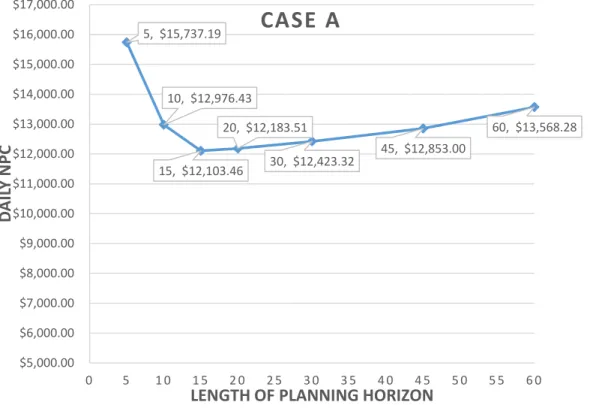
Figure 4-1 Case A Daily NPC Outcomes ... 73

Figure 4-2 Case B Daily NPC Outcomes ... 78

Figure 4-3 Case C Daily NPC outcomes ... 85

Figure 4-4 Comparison of Daily NPC Outcomes ... 88

(6)

Table of Tables

Table 2-1 Primary Research Clusters in SCRM ... 23

Table 3-1 Optimization Model Parameters and coinciding description ... 38

Table 3-2 Set Notation Employed ... 42

Table 3-3 Product Demand Characteristics ... 43

Table 3-4 Average Lead Time from Supplier to Production Facility ... 44

Table 3-5 Raw Material Utilization Summary for Production ... 45

Table 3-6 Summary of Production Rate across Production Facilities ... 45

Table 3-7 Average Lead Time from Production Facility to Warehouse ... 46

Table 3-8 Warehouse Aggregated Product Demand ... 47

Table 3-9 Standard Deviation of Product Demand ... 47

Table 3-10 Product Demand Coefficient of Variation ... 48

Table 3-11 Optimization Model Decision Variables ... 49

Table 4-1 Warehouse Minimum Product Inventories in Days of Expected Demand ... 68

Table 4-2 Minimum Raw Material Inventories in Days of Expected Production ... 69

Table 4-3 Product Inventory Limits at Plant ... 70

Table 4-4 Production System-wide Product Inventory Limits ... 71

Table 4-5 Case A Procurement of Raw Materials ... 75

Table 4-6 Case A Allocation of Production Capacity ... 76

Table 4-7 Case A Distribution Plans ... 77

Table 4-8 Case B Facility Production Set up ... 81

Table 4-9 Case B Procurement of Raw Materials ... 82

Table 4-10 Case B Warehouse Activities ... 83

Table 4-11 Case C Warehouse Activities ... 86

Table 4-12 Allocations of Production Capacity in Production Schedules ... 90

Table 5-1 Shortened Upstream Lead Time with CV ... 94

Table 5-2 Shortened Downstream Lead Time with CV ... 94

Table 5-3 Period One Initial Raw Materials in Transit (Day 1 to Day 20) ... 101

Table 5-4 Period One Beginning Raw Material Inventories (Day 1 to Day 20) ... 102

Table 5-5 Simulated Day One Production Summary ... 102

Table 5-6 Period Two Beginning Raw Material Inventories (Day 2 to Day 21)... 103

(7)

Revision December 6, 2016 Copyright, Liang Xu, 2016 VI

Table 5-9 Period Two Initial Raw Materials in Transit (Day 2 to Day 21) ... 105

Table 5-10 Period One Initial Finished Product Inventory at Facilities ... 106

Table 5-11 Period One Plant to Warehouse Shipment Summary ... 107

Table 5-12 Period Two Initial Finished Product Inventory at Facilities ... 108

Table 5-13 Period One Initial Finished Products in Transit... 109

Table 5-14 Period One Warehouse Product Inventory and Demand Status ... 111

Table 5-15 Period Two Warehouse Product Inventory and Demand Status ... 113

Table 5-16 Replication Two Random Seeds Illustration ... 113

Table 5-17 Period Two Finished Products in Transit (Day 2 to Day 21) ... 114

Table 5-18 Average Daily Product Gross Profit Contribution (H10) ... 116

Table 5-19 Average Daily Product Inventory Costs (H10) ... 117

Table 5-20 Average Daily Raw Material Inventory Costs (H10) ... 117

Table 5-21 Average Daily Plant Idle Costs and Setup Costs (H10) ... 117

Table 5-22 Daily Net Profit Contribution Statement (H10) ... 118

Table 5-23 Daily Net Profit Contribution Statement (H20) ... 119

Table 5-24 Summary of Supply Chain Performance Metrics ... 122

Table 5-25 Scenario One Summary Statistics for Quarterly Product-level SC Metrics in 25 Replications ... 123

Table 5-26 Product Service Level Influential Characteristics ... 125

Table 5-27 Scenario One Drivers of Product Service Level ... 126

Table 5-28 Scenario One Cross Comparison of SC Financial Performance ... 131

Table 5-29 Scenario One Product Level SC Metrics Cross Comparison ... 132

Table 5-30 Scenario One Overall SC Level Duncan Test Results Part I ... 134

Table 5-31 Scenario One Overall SC Level Duncan Test Results Part II ... 135

Table 5-32 Scenario One Overall SC Level Duncan Test Results Part III ... 136

Table 5-33 Scenario One Product Level Duncan Test Results Part I ... 137

Table 5-34 Scenario One Product Level Duncan Test Results Part II ... 138

Table 5-35 Scenario One Product Level Duncan Test Results Part III ... 139

Table 6-1 Scenario Two Cross Comparison of SC Financial Performance with STDOBJ 147 Table 6-2 Scenario Two Summary Statistics for Quarterly Product-level SC Metrics in 25 Replications ... 148

Table 6-3 Scenario Two Cross Comparison of SC Financial Performance ... 150

Table 6-4 Scenario Two Product Level SC Metrics Cross Comparison ... 151

(8)

Table 6-6 Scenario Two Overall SC Level Duncan Test Part II... 154

Table 6-7 Scenario Two Overall SC Level Duncan Test Part III... 155

Table 6-8 Scenario Two Product Level Duncan Test Part I ... 158

Table 6-9 Scenario Two Product Level Duncan Test Part II ... 159

Table 6-10 Scenario Two Product Level Duncan Test Part III ... 160

Table 6-11 Scenario Two Drivers of Product Service Level ... 163

Table B-0-1 Warehouse One Product ROP Results ... 176

Table C-0-1 Case 1 Parameters Value (in days of expected demand) ... 179

Table C-0-2 Case 1 Idles Times, Idle Costs and Setup Indicators ... 180

Table C-0-3 Case 1 Sample of Warehouse Activities ... 180

Table C-0-4 Case 2 Parameters Value ... 181

Table C-0-5 Case 2 Total Product Inventories across Plants ... 183

Table C-0-6 Case 2 Sample of Production and Plant Inventories Summary ... 184

Table C-0-7 Case 2 Sample of Warehouse Activities ... 185

Table C-0-8 Case 3 Parameters Value ... 186

Table C-0-9 Case 3 Total Product Inventories across Plants ... 187

Table C-0-10 Case 3 Sample of Production and Plant Inventories Summary ... 188

Table C-0-11 Case 3 Idles Times, Idle Costs and Setup Indicators ... 189

Table C-0-12 Case 3 Sample of Production and Capacity Utilization ... 189

(9)

Revision December 6, 2016 Copyright, Liang Xu, 2016 VIII

Abstract

Solutions to deterministic optimizing models for supply chains can be very sensitive to the formulation of the objective function and the choice of planning horizon. We illustrate how multi-period optimizing models may be counterproductive if traditional accounting of revenue and costs is performed and planning occurs with too short a planning horizon. We propose a “value added” complement to traditional financial accounting that allows planning to occur with shorter horizons than previously thought necessary.

This dissertation presents a simulation model with an embedded optimizer that can help organizations develop strategies that minimize expected costs or maximize expected contributions to profit while maintaining a designated level of service. Plans are developed with a deterministic optimizing model and each of the decisions for the first period in the planning horizon are implemented within the simulator. Random deviations in demands and in upstream and downstream shipping times are imposed and the state of the system is updated at the end of each simulated period of activity. This process continues iteratively for a chosen number of periods (90 days for this research). Multiple replications are performed using unique random number seeds for each replication. The simulation model generates detailed event logs for each period of simulated activity that are used to analyze supply-chain performance and supply-chain risk. Supply-chain performance is measured with eleven key

(10)

performance indicators that reveal system behavior at the overall supply-chain level, as well as performance related to individual plants, warehouses, and products.

There are three key findings from this research. First, a value-added complement in an optimization model’s objective function can allow planning to occur effectively with a significantly shorter horizon than required when traditional accounting of costs and revenues is employed. Second, solutions with the value-added complement are robust for situations where supply-chain disruptions cause unexpected depletions in inventories at production facilities and warehouses. Third, ceteris paribus, the hybrid multi-period planning approach generates solutions with higher service levels for products with greater revenue per average production-minute, shorter average upstream lead times, and lower coefficients of variation for daily demand.

(11)

Revision December 6, 2016 Copyright, Liang Xu, 2016 10

Chapter 1 Introduction

1.1 Overview

Competition, globalization, shortened product lives and lean production systems have led managers to focus on efficiency and cost reduction in the design and management of supply chains (Ghadge et al., 2012; Tang et al., 2012; Wagner and Bode, 2006; Blackhurst et al., 2005). Greater efficiency, however, does not guarantee greater effectiveness (Heckmann et al. 2015). Implementing various cost effective strategies such as outsourcing, global sourcing, lean production, etc. can reduce safety stocks and time buffers. This exposes enterprises to a higher level of supply chain (SC) risk and acquires even greater significance for organizations involved in multi-mode transportation across international boundaries.

Empirical studies conducted by Hendricks and Singhal (2003, 2005a, b) revealed that SC disruptions can have a significant impact on both shareholder value and operating performance. The Wall Street Journal reported that a Hong Kong port strike in 2013 cost Hongkong International Terminals $644,000 per day (Chiu 2013). Disruption of production for a few days, caused by a custom employees strike, resulted in a million dollar lost for a consumer packaged goods firm located in South America (Schmitt and Singh, 2012). The National Retail Federation (NRF) and National Association of Manufacturers (NAM) revealed that the 10-day stoppage at the West Coast ports in 2002 cost the U.S. economy

(12)

about $1 billion a day and months to recover. Moreover, the NRF-NAM study estimates that a 5-day stoppage at U.S. West Coast ports will cause a daily reduction of GDP by $1.9 billion and affect 73,000 jobs, while a 20-day stoppage will result in a daily loss of $2.5 billion and disrupt 405,000 jobs (Elenstar, 2014).

As the likelihood, frequency and magnitude of SC disruptions increase (Blackhurst et al., 2005; Coleman, 2006; Okubo et al., 2013;Cardoso et al., 2015), supply chain risk management (SCRM) attracts the attention of both researchers and practitioners. Adding to the complexity of supply chain risk management is the fact that strategies needed to mitigate one type of risks may simultaneously increase other risks (Chopra and Sodhi, 2004). Deep relationships with a single supplier, for example, may reduce the risks of receiving incompatible parts but increase the risk of shutdowns due to major disruptions at the supplier’s facilities. Thus, a holistic approach is advocated and organizations should adopt SCRM practices at strategic, tactical, and operational levels. At the tactical and operational levels, SCRM (Hsieh and Wu, 2008; Kara and Kayis, 2004; Pitty et al., 2008; etc.) emphasizes reactive actions to diminish negative impacts once disruptions occur. At the strategic level, SCRM focuses on dealing with risks in a proactive way, thereby reducing or preventing the negative impacts caused by anticipated disruptions (Muckstadt et al., 2003; Rice and Caniato, 2003a; Norrman et al., 2004; Herroelen and Leus, 2005; Kleindorfer and Saad, 2005; Hendricks and Singhal, 2005a; Hendricks et al, 2008; Ji and Zhu, 2008; etc.). When supply chain disruptions or unusual events occur, managerial short-term

(13)

interests may shift, depending on delays in flows of the supply chain. Reactions may cause abnormal patterns in production, distribution and procurement, leading to a dilemma where decisions to optimize performance in a normal time frame may become counterproductive (to be illustrated in Chapter 3 of this dissertation).

Organizations plan based on expectations, often with a rolling horizon whereby they implement decisions according to plan early in the planning horizon, experience events that cause the state of the system to differ from expectations, and revise the plan as new information becomes available. When planning with a rolling horizon, organizations confront the question of how long the horizon should be. This question has been ignored in most supply chain management (SCM) studies that employ optimization models for tactical and operational decisions (e.g., Ciarallo et al., 1994; Wang and Gerchak, 1996; You et al., 2009; Cardoso et al., 2015 etc.). The first question we address in this dissertation is therefore:

Q1: What rolling horizon length should be adopted in order to achieve higher SC performance for a given objective function and performance metrics?

At face, it seems that to consider the consequences of decisions connected with activities in the supply chain, the planning horizon would need to encompass the longest lead time for procurement of materials, the production

(14)

cycle times at the manufacturing facilities, and the longest lead time downstream for goods to reach consumers. This seems necessary to avoid decisions from short-term optimization that could harm long-term performance. A planning horizon that encompasses the longest lead times upstream and downstream plus the production cycle time may not be practicable, however, especially for organizations managing international logistics and supply chains. We therefore experiment with a value-added planning objective that enables an organization to recognize the effects of decisions for which the benefits and costs will accrue beyond the planning horizon. We explore the use of such value-added planning objective in a stochastic environment with discrete-event simulation. We apply the research model on a rolling horizon over 90 days, generate 11 key performance measures, impose normal SC variations (product demand, upstream and downstream lead time), and analyze resulting SC performance via different combination of the length of the planning horizon and the approach in the objective function to address our second research question:

Q2: Can a “value-added” complement to the SCM objective function mitigate the sub-optimization that occurs when the planning horizon is shorter than the time required to capture the effects of all relevant events (procurement, production and deliveries) upstream and downstream?

(15)

After addressing Q2, we next consider the effects of uncertainty by imposing random disruptions that result in inventory shortages, apply the same multi-period SC planning settings (a rolling horizon over 90 days and different combination of the planning horizon and the approach in the objective function), and evaluate the resulting SC performance on the same 11 key metrics to address our third research question:

Q3: Does any advantage derived from the value-added complement to the objective function persist when SC disruptions occur?

After recognizing the benefits of the value-added complement to the objective function, we compare results derived from addressing Q2 and Q3 to address our fourth and fifth research question:

Q4: How sensitive is SC performance to the choice of planning horizon and addition of the value-added complement to the objective function?

Q5: What product characteristics are associated with the differential service levels that result from application of the SC optimization model on a rolling horizon?

1.2 Research Methodology

Analytical modeling is employed by researchers and practitioners to support managerial decision making while recognizing interdependencies of

(16)

activities in a supply chain. These models can be even more beneficial when probabilistic and/or random variations are incorporated. To capture the stochastic elements in the SC, this research presents a simulation model with an embedded optimizer to address the research questions. This hybrid model is constructed on the Statistical Analysis System (SAS) 9.4 platform.

The hybrid model presented in the research is aimed at solving multi-period SC planning problems. Each replication consists 90 days of activity with a rolling optimization horizon. Solutions for the chosen planning horizon at the end of each revision period are extracted and saved in a dataset that stores in a specified SAS library. The simulation model reads the extracted solutions from the SAS library and updates the dataset with stochastic demands and stochastic transit times for flows in the supply chain network during the revision period. It schedules arrivals of goods and materials accordingly and imposes the results as boundary conditions for re-solution of the planning model. Then the optimization model reads the information from the updated dataset as the new initial conditions and solves the problem for the chosen planning horizon. This iterative process continues until it reaches the last day in the experimental period and last replication. Figure 1-1 illustrates the interactive process of the hybrid model.

(17)

Revision December 6, 2016 Copyright, Liang Xu, 2016 16 Figure 1-1 Interaction Between Simulation and Optimization

Statistical analysis is performed at the end to generate insights and provide foundations for research findings.

1.3 Research Outline

The remainder of this dissertation is presented in five chapters. Chapter 2 contains a review of the relevant literature and identifies the literature gaps which motivate the purposes of this research. Chapter 3 presents the design and methodological underpinnings of the deterministic optimization model. Chapter 4 illustrates characteristic behaviors of the analytical model. Chapter 5 addresses Q1 and Q2. Q1: What rolling horizon length should be adopted in order to achieve higher SC performance for the given objective function and performance metrics? Q2: Can a “value-added” complement to the SCM objective function

(18)

mitigate the sub-optimization that occurs when the planning horizon is shorter than the time required to capture the effects of all relevant events (procurement, production and deliveries) upstream and downstream? This is investigated through scenario one under the circumstances that there are no major disruptions in the supply chain. In Chapter 6, section 6.2 addresses question Q3: Does any advantage derived from the value-added complement to the objective function persist when supply chain disruptions occur? This is investigated via scenario two where outages occur randomly with 20% of product-warehouse combination which represent disruptions or unusual events that deplete product inventories at the warehouse. In section 6.3, SC performance from scenario one and scenario two are compared to address Q4: How sensitive is SC performance to the choice of planning horizon and addition of the value-added complement to the objective function? Product service level derived from scenario one and scenario two are evaluated to address Q5: What product characteristics are associated with the differential service levels that result from application of the SC optimization model on a rolling horizon? Chapter 7 summarizes the research findings, provides managerial insights, discusses the limitations of the research, and identifies areas for future research.

(19)

Chapter 2 Literature Reviews

2.1 Supply Chain Risk

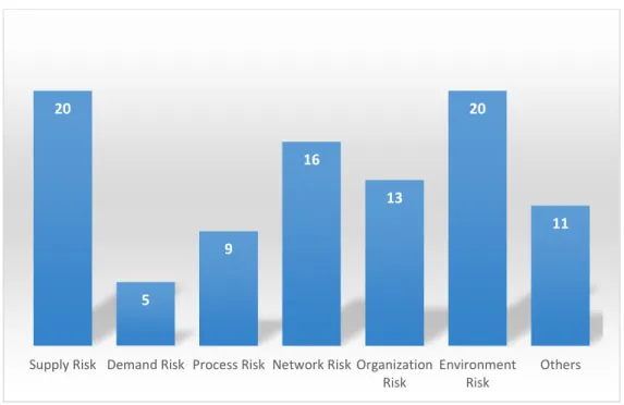
General sources of SC risk that have been discussed in the academic literature are summarized in Figure 2-1. They can be classified as Supply Risk, Demand Risk, Process Risk, Network Risk, Organizational Risk, and Environmental Risk. The numbers in Figure 2-1 indicate the number of subtopics identified in each category in this research. Details for each of the subtopics are provided in Appendix A. Particular sources of SC risk include market capacity (Zsidisin, 2003), uncertain variable cost (Tang, 2006 b; Bilsel and Ravindran, 2011), resources (talent, technology, and capital) risk (Ghoshal, 1987), product variety (Thun and Hoenig, 2011), and general SC risk caused by single sourcing, globalization, Just-In-Time production, centralized distribution and production (Juttner, 2005; Thun and Hoenig, 2011).

(20)

Figure 2-1 Major Sources of SC Risk

Depending on the magnitude of negative impact, SC risk may be described as “disruption”, “disturbance”, “crisis”, “vulnerability”, “uncertainty”, “adverse events”, “disaster”, “peril”, “glitch”, “hazard”, and “perturbations” (Harland et al., 2003; Christopher and Peck, 2004; Christopher and Lee, 2004; Blackhurst et al., 2005; Hendricks and Singhal, 2005a; Tang, 2006a, b; Wagner and Bode, 2006; Ghadge et al., 2012; Wu et al., 2007; and Azevedo et al., 2008). Most of the literature discusses SC risk in two dimensions: probability and severity (March and Shapira, 1987; Mitchell, 1995; Harland et al., 2003; Kleindorfer and Saad, 2005; Wagner and Bode, 2008; Manuj and Mentzer, 2008; Thun and Hoenig, 2011; Wang, 2014; etc.). More recent works argue that the duration of SC risk should also be considered (Klibi and Martel, 2012; Schmitt &

20 5 9 16 13 20 11

Supply Risk Demand Risk Process Risk Network Risk Organization Risk

Environment Risk

(21)

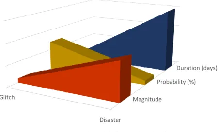
Singh, 2012) as an important dimension. On one hand, minor disruptions in production due to machine breakdowns may be considered as a glitch and probably ignored due to small magnitude associated. Major disruptions, on the other hand, such as those caused by a tsunami can be classified as a “disaster” because they may affect an entire industry or economy. Although SC risk has a multifaceted and multidimensional construct (Wagner and Bode, 2006), in this research, probability, magnitude and duration are used to capture key characteristics of a SC risk. Using these three dimensions, Figure 2-2 illustrates the differences between aforementioned SC risks.

Figure 2-2 Key Factors to Describe SC Risk

2.2 Supply Chain Risk Management

If achieving greater SC efficiency through various cost reduction strategies is important for organizations to increase competitiveness and

Magnitude

Probability (%) Duration (days)

Glitch

Disaster

(22)

improve performance, then ensuring the continuous flows of goods, services, and related information, which is the effectiveness of a SC, is equally important. However, assuring the effectiveness of a SC is a challenging task, and even more so for a global supply chain (GSC). As an organization spans national boundaries to further exploit opportunities and reduce costs, the SC becomes longer and more complex. Managing a GSC requires the assistance of advanced information technology. Decision makers face challenges in collaborating with SC partners that have different cultural backgrounds, speak different languages, and reside in different time zones. Companies experience changes in governmental regulations, customs delays, varying exchange rates, strikes, and political instability.

Unexpected disruptions can result in stockouts and the inability to meet customer demand, decrease the efficiency of SCs (Blackhurst et al., 2005), and have negative effects on stock prices (Hendricks and Singhal, 2005a). Despite all these challenges, there is evidence that a GSC presents opportunities that can be explored with good risk management. Hauser (2003) posits that risk adjusted supply chain management (SCM) leads to improved financial performance and competitive advantage. An empirical study conducted by Thun and Hoenig (2011) in the German automotive industry revealed that integrated SCRM tends to improve the performance of a SC, as companies with the lowest degree of SCRM, on average, had the lowest values for all performance criteria.

(23)

Narasimhan and Talluri (2009) view SCRM as “a strategic management activity in firms given that it can affect operational, market and financial performance of firms” and argue that the essence of SCRM is to optimally align organizational processes with decisions to exploit opportunities while simultaneously minimizing risk (Miles et al., 1978; Venkatraman and Camillus, 1984). However, this perspective on SCRM focuses on individual organizations while omitting the collaboration with SC partners to cope with SC risks. Tang (2006 b) defined SCRM as “the management of SC risks through coordination or collaboration among the supply chain partners so as to ensure profitability and continuity”. The importance of coordination and collaboration in SCRM is also stressed by Juttner et al. (2003), Norrman and Lindroth (2004), and Olson and Swenseth (2014).

Although SCRM is a growing research area, Sodhi et al. (2012) stated that SCRM can be very subjective with varying definitions and interpretations among researchers. Focusing on quantitative approaches in SCRM, this research believes that SCRM should be integrated into modern SCM with the primary responsibility to assure the continuous flows of goods, services, and related

(24)

2.3 Quantitative research in Supply Chain Risk Management

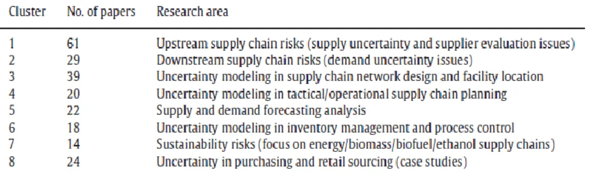
Various methodologies have been applied in managing SC risks. Fahimnia et al. (2015) identified eight primary research clusters (Table 2-1) in SCRM.

Table 2-1 Primary Research Clusters in SCRM

(Source: Fahimnia et al., 2015)

Among these clusters, “uncertainty modeling in tactical/operational supply chain planning” is the most relevant one to this research. Lead papers in cluster 4, plus additional quantitative approaches in SCRM have been reviewed in this research.

2.3.1 Supply Chain Planning

Deleris and Erhun (2005) developed a Monte Carlo simulation model to assess the impact of SC disruptions on network flow. With an interest in system downtime and recovery time, Schmitt and Singh (2012) used Arena to simulate a multi-echelon consumer packaged goods SC to examine how risk flows in the SC

(25)

and how disruptions affect each node in the SC network. This research, using customer fulfillment as a performance metric, illustrates that SC risk assessment at the network level can best reveal the true level of risk exposure. They further show how flexibility through redundancy can increase SC resilience and reduce the risk of failure. Redundancy is realized through buffer inventories and backup capacities. The cost structure (holding costs of raw materials, work-in-process, and finished goods) determines where buffer inventories should be positioned and the source of disruptions in the SC network affects the selection of appropriate mitigation strategies. Importantly, the research demonstrates that the magnitude of SC disruptions varies through time and the impacts can be amplified and outlast the disruptions themselves as events propagate through the SC.

You et al. (2009) proposed a stochastic model that incorporates demand and freight rate uncertainty to examine the tradeoffs between cost and risk in multi-period planning. The research revealed that for different risk management methods (managing the variance, the variability index, the probabilistic financial risk, and the downside risk), total expected cost will increase after risk management. Bode et al. (2011) confirmed that buffering (building safeguards such as inventory) and bridging (collaborating with SC partners) are two generic strategies adopted by firms to cope with SC risk. Their empirical study revealed that organizations regard these two strategies as equally effective alternatives. Cardoso et al. (2015) developed a MILP model for SC design and planning to

(26)

investigate system resilience associated with different SC structures when considering demand uncertainty in a fixed time period (t=3). Their research concluded that, depending on the existing SC network structure, adding redundancy does not always lead to a more resilient SC.

Lee and Kim (2002) adopted a hybrid approach, iterating between a deterministic optimization model and a discrete-event simulation model, to address the integrated production-distribution problems with consideration of production and distribution uncertainty. Operation time uncertainties, including machine and vehicle breakdown, queuing, and transportation delays, were captured by the simulation model. To hedge against variations in demand, Lin and Chen (2009) developed a stochastic model to explore the benefit of flexibility in coordinated replenishment and shipment policies for a fixed planning horizon (30 days). Sabri and Beamon (2000) developed sets of model to simultaneously address strategic and operational SC planning problems. A deterministic model (MILP) was constructed for strategic planning. To incorporate uncertainties in production, delivery, and demand, a stochastic model was developed at the operational level. The research adopted an iterative approach between deterministic and stochastic models to assist in strategic and operational planning. Sodhi (2005) presented a deterministic model and a stochastic model to solve the replenishment schedule for an electronics company. He used information from these two models as a guide for managers to reallocate capacity among different products to mitigate inventory and

(27)

demand risk. A stochastic model was developed by Leung et al., (2006) to address the production planning problem with consideration of uncertain demand for a given 3-month planning horizon. Variation in demand is not directly incorporated into the model. Instead, uncertain demand is realized through changes in probability distributions of economic scenarios.

In order to achieve desired customer service level in all demand regions, Jung et al., (2004) developed sets of models to investigate safety stocks needed to cope with demand uncertainty for a given planning period (3 months). A stochastic planning and scheduling model incorporates buffer inventories to deal with demand uncertainty, while simulation with an embedded optimization model was used to address safety stock levels needed in order to achieve desired customer service level. The planning and scheduling problem was employed with a rolling horizon (increase one period at a time until the end of planning period), however, the length of the rolling planning horizon is not clarified in their research. Instead, their assumption pertains to the length of the rolling planning horizon considers downstream longest lead time (delivery from each production facility to each customer takes less time than the chosen horizon). Although the model proposed in this research is robust, it is almost impossible to allow any tactical analysis to react to SC disruptions because of the computation time required (100 hours).

Wang and Gerchak (1996) developed a stochastic model to investigate the production planning problem with consideration of uncertain production

(28)

processes and uncertain demand. The research revealed (not surprisingly) that for a multi-period production planning problem, the optimal policy depends upon the initial inventory level at each period. Schmitt and Singh (2009) presented a simulation model (Monte Carlo with Arena) to investigate the impact of disruptions on SC and assess strategies for coping with SC risk in pursuit of a targeted service level. Their research showed how customer service depends on inventory levels in the system at the beginning of a disruption and the nature of uncertainty in demand and production operation. They assert that it is important to monitor and evaluate SC risk through time.

2.3.2 Correlations among Supply Chain Risk Sources

Monte Carlo simulation was applied to investigate outsourcing risks in the SC by Lee et al. (2012). The research revealed that although total average lead time and total average SC costs were both reduced after outsourcing, the variation of cost was increased due to exposure to risk or uncertainty. Bode and Wagner (2015) did an empirical study to investigate the relationship between conceptualized upstream SC complexity and the frequency of disruptions experienced by buying firms. These conceptualized structures are horizontal complexity (number of direct suppliers), vertical complexity (number of ties), and spatial complexity (global sourcing). Their findings suggested that each of aforementioned dimensions of upstream SC complexity is a source of disruption risk.

(29)

Wu and Olson (2008) proposed three different models to assist in vendor selection with consideration of risks: chance constrained programming, data envelopment analysis, and multi-objective programming. Risks were incorporated with probability distributions and risk profiles were generated through Monte Carlo simulation, then embedded into the aforementioned models. Kull and Closs (2008) developed a discrete-event simulation model to investigate the disruption impacts associated with second-tier supply failure. Multi-regression analysis was used to assess the impact of inventory level and ordering policy on supply risk. The researchers concluded that ordering policies can have significant impact on firm’s exposure to supply risk, and that inventory in the system is not an adequate indicator of SC resilience. Empirical studies conducted by Wagner et al., (2009, 2011) focused on investigating default dependence between suppliers and concluded that such interdependencies can have significant detrimental impacts on the buying firm. Costantino and Pellegrino (2010) developed a Monte Carlo simulation model to explore the tradeoffs between single sourcing and dual sourcing and indicated that the additional costs of using than one supplier may be offset by reduction in supply risk. More importantly, their research stated that if the default probability of all suppliers is correlated, managers should consider having an additional supplier in a foreign country or carrying more buffer inventory. Guertler and Spinler (2015) used Monte Carlo simulation to investigate the interrelationships among various supply risks mentioned in the literature and concluded that such

(30)

interdependencies can significantly affect the total risk originated from SC upstream.

Tsiakis et al. (2001) developed a mixed integer linear programming (MILP) to assist in designing a multiproduct, multi-echelon SC network with consideration of demand uncertainty. Vaagen and Wallace (2008) developed a multidimensional stochastic optimization model to assess the impact of uncertainties and demand correlations on system performance for fashion SCs. The research concluded that ignoring demand correlations of fashion products can lead to inferior trade-offs between risk and expected profit. Ciarallo et al. (1994) constructed a stochastic model to solve the production planning problem with consideration of uncertain demand and uncertain capacity. The variation in demand and uncertain production capacity were captured by random variables with a general distribution. The research indicated that an order-up-to inventory policy may be used effectively for multiple-period production planning problem but suggested that a more realistic production planning model should consider nonzero correlations between random demands in different periods. Focusing on SC design problems, Azaron et al. (2008) developed a stochastic model with consideration of uncertain costs in production. The objectives were to minimize the expected total costs, the variance of total cost, and the financial risk when configuring a SC. Sets of scenarios with given probabilities of occurrence were considered. Demands, supplies, processing costs, transportation costs, and shortage and capacity expansion costs were modeled as random variables. The

(31)

study illustrated correlations between the expected total SC cost and financial risk. Lim et al. (2005) adopted a hybrid approach, iterating between genetic algorithm (GA) and simulation, to solve a distribution planning problem. The GA is used to find near optimal solutions, while simulation captures uncertainty associated with machine and transportation vehicles. Moreover, research conducted by Lium et al. (2007) via stochastic programming revealed that the correlation structure of demand (positive, mixed, negative) affects the optimal truck routes (less-than-truckload).

Petrovic et al. (1998) developed fuzzy models and a simulation model, to investigate the tradeoffs between stock levels, order quantities, and total delivery costs. Uncertain demand and uncertain supply of raw materials were modeled using fuzzy sets. Simulation was used to assess the impact of decisions derived from fuzzy models on system performance. Petrovic (2001) constructed sets of models to analyze SC behavior and performance with consideration of uncertainties. Uncertain demand, uncertain raw materials supply, and uncertain lead time were again modeled using fuzzy sets. Simulation was used to assess the impact of decisions derived from fuzzy models on system performance. However, correlations among demands were not considered in Petrovic et al., 1998 and Petrovic, 2001.

Giannakis and Louis (2011) proposed a conceptual multi-agent based framework to facilitate SCRM. Okubo et al. (2013) used scenario-based simulation to investigate the impact of disruptions on a given SC and evaluate

(32)

the effectiveness associated with different restoration plans (considering time to restore full capacity versus time to restart production). Talluri et al. (2013) used discrete-event simulation to test the appropriateness and effectiveness of conceptual SCRM framework proposed by Chopra and Sodhi (2004). The study revealed that the appropriateness and effectiveness of risk mitigation strategies are contingent on the internal and external environments. Their research suggested that SCRM needs to consider risk category, risk source, and SC configuration and there is no one-size-fits-all strategy. Their research does not consider the correlations of SC risk sources and does not allow multiple risks or strategies to interact simultaneously. Tomlin (2009) developed a stochastic model to investigate various supply chain risk mitigation strategies (SCRMS) to cope with the supply disruption with considerations of uncertainties derived from upstream and downstream activities. The research concluded that a supply diversification strategy is preferred to contingent sourcing if demand risk is high, while contingent sourcing becomes more effective than supply diversification if supply failure probability increases. Furthermore, the study revealed that demand switching tactics can be used to cope with variations in demand. However, if products are sourced from the same set of suppliers, demand switching is not an effective antidote to supply risk.

With various perspectives on SCRM, researchers have recognized that correlations among sources of risk impinge on sourcing strategies (Wagner et al., 2009, 2011; Costantino and Pellegrino, 2010), vehicle routing solutions (Lium et

(33)

al., 2007), and financial performance (Vaagen and Wallace, 2008). However, analytical models (such as stochastic programming) that incorporate risk, generally assume that supply chain risk components, such as variation of demand in different markets, transportation delays, etc. are independent of each other (Ciarallo et al., 1994; Wang and Gerchak, 1996; Sodhi, 2005; Wu and Olson, 2008; Lin and Chen, 2009; Schmitt and Singh, 2012; Cardoso et al., 2015 etc.). This may cause a significant underestimation of the impact of adverse events (Zhang and Li, 2010; Liberatore et al, 2012).

2.4 Supply Chain Event Management

An important aspect of risk mitigation involves dealing with adverse events when they occur. Following Bearzotti et al, 2012; Giannakis and Louis, 2011; Bodendorf and Zimmermann, 2005; and Otto 2003, we call this supply chain risk event management (SCEM). It is the combination of supply chain risk mitigation strategies and supply chain risk event management that determines the ultimate performances of the system. Examples of actions which might be taken in response to adverse events occurred in the SC are the use of overtime or alternative supplies of raw materials and components when production must be intensified. Such reactive actions may include the use of faster (usually more expensive) modes of transportation when there is an urgent need for supplies at manufacturing facility, goods at warehouse, or final delivery to a customer.

(34)

Taking reactive actions in a timely manner is crucial for organizations to recover and, most importantly, to survive (Simchi-Levi, 2015).

2.5 Summary

Because the initial state of the system directs the optimal policy, it is essential to capture changes in the state of the system at the beginning of each period when dealing with multi-period SC planning. The importance of adopting rolling planning horizon and adequately updating the initial conditions to capture changes in the state of the system can never be overstressed. However, regardless the consideration of uncertainties, there has been limited research employing a rolling planning horizon and capturing changes in the state of the system to solve multi-period SC planning problems. Meanwhile, it is generally recognized that short term optimization can actually hurt long term performance. But, when disruptions or unusual events occur, depending on the magnitude and the duration of the risk events, SC may experience abnormal patterns in procurement, production and distribution etc., and managerial short-term interests may also shift. The same SC planning toolbox or analytical model utilized before the risk events may be counterproductive and unable to reveal the true SC performance. A robust analytical toolbox requires excessive time to generate results (100 hours in Jung et al., 2004) and is likely unable to satisfy managerial short-term needs to cope with risk events occurred, especially when

(35)

reaction in a timely manner is the essence to mitigate risk effects. However, rarely discussed in the literature is the different approach in the objective function of the analytical models to deal with such a dilemma. Last but not least, in the field of SCM, sporadic studies utilize multi-criteria to assess the overall SC performance and assist managerial decision making by providing the “whole picture” (upstream and downstream) of the SC.

This dissertation investigates the effects of using a combination of strategies for SCRM and SCEM by employing a discrete-event simulation model with an embedded optimizer. A rolling horizon planning with consideration of the initial conditions for each period is adopted to solve multi-period SC planning problems. The hybrid model produces 11 key SC performance measures to assist managers in making procurement, production and distribution decisions and assessing the effects of different risk-mitigation strategies such as redundancy and flexibility. We propose a value-added complement to traditional deterministic objective functions to improve SCRM and assess its robustness with the hybrid model. We investigate how changes in the length of rolling planning horizons and the approach in analytical model’s objective function for developing and implementing production schedules may affect system performance. Meanwhile, the hybrid approach proposed in this research is intended to meld the strengths of mathematical optimization (pursuit of a goal while adhering to constraints) and simulation (incorporating uncertainty) in an analytically tractable manner.

(36)

Chapter 3 Analytical Model

In the supply chain management field, hybrid approaches which combine simulation and optimization are gaining more attention. Simulated decisions can be formed with help from optimizing models and constraints imposed in the optimization process can be guided by simulation results. Beginning with an integrated simulation and optimization model constructed on the Statistical Analysis System (SAS) platform by Smith et al. (2016), this research incorporates additional elements of upstream activities, sets production system-wide inventory level for each product across all plants, and experiments with different methods of establishing production priorities (Note that the terms “plant”, “facility”, and “production facility” will be used interchangeably in the remaining of this research).

3.1 Model analysis framework

This research studies a three-echelon supply chain for bulk products that are distributed through warehouses in several different regions. The supply chain under investigation is predefined and has m suppliers, n production facilities, p products, and w warehouses. Customers’ demands are aggregated and allocated to the warehouses. The locations of suppliers, production facilities, and warehouses are hypothetically given and the transportation of raw materials and finished goods is assumed to be done by third-party logistics (3PL) providers

(37)

(thus avoiding the issues of consolidating shipments and related delay due the shipment consolidation process). Research data were adapted from the literature (Tsiakis et al., 2001) with amendments made to accommodate the purposes of this research. Figure 3-1 illustrates the supply chain structure examined by this research.

Figure 3-1 Research Supply Chain Structure

With an interest in maximizing net profit contribution, major decisions resulted from the optimization model in each planning period include procurement, production, and distribution plans. Buffer inventories (raw materials, finished goods at plants and products at warehouses) are built into supply chain as part of the risk mitigation strategies. Supply chain risk event management is represented by allowing finished goods to be shipped directly to customers when shortages occur at customer service centers (warehouses) or by

(38)

adding additional shifts when production must be intensified (possibly due to disruptions that have occurred in the supply chain).

3.2 Model description

The analytical model is developed with the following assumptions: 1) The managerial goal is to maximize net contribution to profit.

2) The profit contribution net of shipping costs is realized when customer demand is satisfied from the warehouses or directly from the plant.

3) Inventory replenishment is recognized at the end of each business day. 4) Aggregate customer demands for products are registered at the beginning of

each day at the warehouses.

5) Suppliers who provide the same raw material are geographically separated (and therefore subject to different disruption risks).

6) Each production facility can produce all products, ship products to all warehouses, and perform alternative delivery of finished goods via expedited shipping to satisfy customer demand as alternatives to deliveries from warehouses.

7) Customer demand of products is aggregated and assigned to designated warehouse every day. Alternative deliveries from other warehouses are not considered in this research.

(39)

Description of the notation used in this research is presented in the following table.

Table 3-1 Optimization Model Parameters and coinciding description

Parameter Description

mrRrPp

Units of raw material r required to produce one unit of product p

mininvPpFf

Minimum inventory of product p desired at production facility f

maxinvPpFf

Maximum inventory of product p desired at production facility f

mininvRrFf

Minimum inventory of raw material r desired at production facility f

maxinvRrFf

Maximum inventory of raw material r desired at production facility f

ShtPenaltyRrFf

Daily penalty ($ per unit) for shortage of raw material r inventory at production facility f

ShtPenaltyPpFf

Daily penalty ($ per unit) for shortage of product p inventory at production facility f

ShtPenaltyPpWw

Daily penalty ($ per unit) for shortage of product p inventory at warehouse w

(40)

OvrPenaltyRrFf

Daily penalty ($ per unit) for excess raw material r inventory at production facility f

OvrPenaltyPpFf

Daily penalty ($ per unit) for excess of product p inventory at production facility f

OvrPenaltyPpWw

Daily penalty ($ per unit) for excess of product p inventory at warehouse w

mininvPpWw

Minimum inventory of product p desired at warehouse w (including outstanding orders)

maxinvPpWw

Maximum inventory of product p desired at warehouse w (including outstanding orders)

dempwhsew

Assigned aggregated average daily demand for product p at warehouse w

shiptimeFfWw

δ (f, w)

Shipping time (days) from production facility f to warehouse w

shiptimeSsFf

θ (s, f)

Shipping time (days) from supplier s to production facility f

spcFf

Production setup costs at production facility f incurred each day that production occurs (including idle cost associated with set up time)

pcPpWw

Unit profit contribution of product p delivered from warehouse w

(41)

scPpFfWw

Supply cost per unit of product p from production facility f to warehouse w (including variable production cost at

production facility f and shipping cost from production facility f to warehouse w, but excluding raw material and goods in transit costs)

scRrSsFf

Supply cost per unit of raw material r from supplier s to production facility f (including ordering and shipping costs, but excluding raw material in transit costs)

scPpWw

Shipping cost per unit of product p from warehouse w to customer

icPpFf

Inventory carrying cost for finished product p at production facility f

icRrFf

Inventory carrying cost of raw material r at production facility f

itcPpFfWw

Unit cost of carrying product p in transit from production facility f to warehouse w

itcRrSsFf

Unit cost of raw material r in transit from supplier s to production facility f

acPpFfWw

Unit cost of alternative supply from production facility f for product p at warehouse w

(42)

opcostPpWw

Unit opportunity cost of lost sales for product p at warehouse w

DemPpWwDd Demand for product p (units) at warehouse w on day d

sutimePpFf Product p production setup time at production facility f

idlePenFf Idle penalty cost per hour at production facility f

MXprodFf Maximum daily throughput (units) at production facility f

minsysinvPp

Desired minimum system inventory of product p (across all production facilities)

maxsysinvPp

Desired maximum system inventory of product p (across all production facilities)

(43)

Revision December 6, 2016 Copyright, Liang Xu, 2016 42 Table 3-2 Set Notation Employed

Set Description

R{r} Set of raw materials

S{s} Set of suppliers

F{f} Set of production facilities

P{p} Set of products

W{w} Set of warehouses

D{d} Set of days in planning horizon

SR{r} Set of suppliers for raw material r

RP{p} Set of raw materials used in producing product p

PF{f} Set of products produced in production facility f

PR{r} Set of products require raw material r for production

RF{f}

Set of raw materials used in producing products at production facility f

PW{w} Set of products distributed through warehouse w

WP{p} Set of warehouses to which product p is delivered

DRMS {r, s, f}

Set of days on which raw material r from supplier s is scheduled to arrive at production facility f

DFGS {p, f, w}

Set of days on which product p from production facility f is scheduled to arrive at warehouse w

(44)

Parameters are set for individual products to allow experiments from which conclusions may be generalized according to product type (where product type is characterized by product value, level of demand, and variability of demand). As Fisher (1997) indicated that the supply chain strategy of a product must be aligned with the demand characteristics of that product and Talluri et al. (2013) stated that more realistic supply chain risk mitigation strategies should consider demand variations. Among all six products produced across production facilities, product 1 (P1) and product 2 (P2) have high demand, product 3 (P3) and product 4 (P4) have medium demand, while product 5 (P5) and product 6 (P6) share low demand. However, the variability in demand differs among products. Table3-3 summarizes demand characteristics of all six products considered in this research and presents unit profit contribution associated with each product.

Table 3-3 Product Demand Characteristics

Product Demand Demand

Variation Unit Profit Contribution P1 High High $9.15 P2 High Low $8.26 P3 Medium High $11.44 P4 Medium Low $10.48 P5 Low High $28.85 P6 Low Low $26.78

(45)

Three different raw materials are consumed at production facilities to produce all products. Each raw material has two suppliers with one supplier offering a shorter lead time at a higher cost than the other. Supplier 1 (S1) and supplier 2 (S2) provide raw material 1 (R1), supplier 3 (S3) and supplier 4 (S4) supply raw material 2 (R2), and supplier 5 (S5) and supplier 6 (S6) sell raw material 3 (R3). Table 3-4 presents information about average lead time and standard deviation of lead time from supplier to production facility (F1 to F3 denotes production facility 1 to production facility 3 correspondingly).

Table 3-4 Average Lead Time from Supplier to Production Facility

Supplier Average Lead Time

Standard Deviation of Lead Time F1 F2 F3 F1 F2 F3 S1 10 12 15 1 2 2 S2 16 17 20 2 3 5 S3 9 7 15 1 1 2 S4 13 11 20 2 2 5 S5 10 13 10 1 2 1 S6 16 17 15 2 3 3

P1 and P2 require R1, P3 and P4 require R2, and P5 and P6 require R3. However, units of raw materials required to produce each unit of product can be different. Material requirements for production of all products are given in Table 3-5.

(46)

Table 3-5 Raw Material Utilization Summary for Production

Product Raw Material

Consumption Material Requirements

P1 R1 1.6 P2 R1 1.5 P3 R2 2.5 P4 R2 2 P5 R3 3 P6 R3 3

Table 3-6 Summary of Production Rate across Production Facilities

Product Production Rate (unit/hour)

F1 F2 F3 P1 138 126 145 P2 161 146 168 P3 70 81 77 P4 80 92 88 P5 52 50 45 P6 58 55 50

Although products can be produced at different plants, production capacity differs among products and plants. Production facilities can ship products to all warehouses with varying costs and lead time. Table 3-6 illustrates the production rate (unit per hour) across production facilities and Table 3-7 provides information about average lead time and standard deviation of lead time from production facility to warehouse (WH1 to WH6 denotes warehouse 1

(47)

Information presented in Table 3-6 and Table 3-7 indirectly indicates that the unit supply cost of products from production facility to warehouse are set to depend on the combination of profit contribution of individual products, lead time from plant to warehouse, and the level of economies of scale at each individual plant.

Table 3-7 Average Lead Time from Production Facility to Warehouse

Average Lead Time

Standard Deviation of Lead Time F1 F2 F3 F1 F2 F3 WH1 7 9 15 2 2 3 WH2 7 10 17 2 3 4 WH3 8 7 17 2 2 5 WH4 9 7 19 3 2 6 WH5 13 15 7 5 5 2 WH6 15 15 8 5 6 2

The supply chain is generally demand driven. Information of product demands collected from warehouses dictates the quantity that the production scheduling model should produce, units of products to ship, and the amount of raw materials to purchase. Meanwhile, production of products, delivery of products, and procurement of raw materials take into consideration the minimum inventories of raw materials to maintain at plants, minimum inventories of finished products to maintain at plants, minimum system-wide

(48)

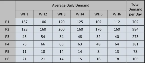
inventories of finished products, and minimum inventories of finished goods at warehouses. Table 3-8 and table 3-9 summarize the aggregated demand information through warehouses in this research. Table 3-10 presents coefficients of variation for demands of products at warehouses. As some products exhibit high coefficients of variation, these product demands are being truncated in the simulation model to avoid any negative values.

Table 3-8 Warehouse Aggregated Product Demand

Average Daily Demand

Total Demand per Day WH1 WH2 WH3 WH4 WH5 WH6 P1 137 106 120 125 102 112 702 P2 128 160 200 160 176 160 984 P3 45 54 54 48 32 40 273 P4 75 66 65 63 48 64 381 P5 11 18 14 14 8 13 78 P6 21 21 14 15 16 18 105

Table 3-9 Standard Deviation of Product Demand

Standard Deviation of Daily Demand

WH1 WH2 WH3 WH4 WH5 WH6 P1 21 16 18 19 15 17 P2 6 8 10 8 9 8 P3 16 19 19 17 12 14 P4 19 17 17 16 12 16 P5 6 9 7 7 4 7 P6 9 9 6 6 7 8

(49)

Revision December 6, 2016 Copyright, Liang Xu, 2016 48 Table 3-10 Product Demand Coefficient of Variation

Product Demand Coefficient of Variation

WH1 WH2 WH3 WH4 WH5 WH6 P1 0.15 0.15 0.15 0.15 0.15 0.15 P2 0.05 0.05 0.05 0.05 0.05 0.05 P3 0.36 0.35 0.35 0.35 0.38 0.35 P4 0.25 0.26 0.26 0.25 0.25 0.25 P5 0.55 0.50 0.50 0.50 0.50 0.54 P6 0.43 0.43 0.43 0.40 0.44 0.44 3.3 Model construction

Daily production at plants, shipments to warehouses, and deliveries to customers are planned with consideration of production capacities across plants, lower and upper inventory limits at plants and in warehouses, transit times to warehouses, and the possibility of expedited shipping from production facilities directly to the customer (at higher cost) or accepting lost sales in the event of stockouts at the warehouses. A mixed-integer mathematical programming model (with options of planning over different horizons considering current system status, expected future demands, shipping times etc.) is employed to determine “optimal” allocations of production capacity each day and shipments to warehouses from which customer demand is satisfied. Decision variables are presented in table 3-10, followed with optimization model’s objective and constraints.

(50)

Table 3-11 Optimization Model Decision Variables

Decision Variables

Description

ProdPpFfDd Units of product p produced at production facility f at the end

of day d

USPpFfDd Units short of safety stock of product p at production facility f

at the end of day d

OSPpFfDd Units over max desired inventory of product p at production

facility f at the end of day d

ShpPpFfWWDd Units of product p shipped out of production facility f to

warehouse w at the end of day d

ItsPpFfWWDd Units of product p in transit and scheduled to arrive at

warehouse w from production facility f at the end of day d

USRrFfDd Under-stock (shortage from reorder point) of raw material r at

production facility f at the end of day d

OSRrFfDd Over-stock (above max desired inventory) of raw material r at

production facility f at the end of day d

ShpRrSsFfDd Units of raw material r shipped out of supplier s to production

facility f at the end of day d

ItsRrSsFfDd Units of raw material r in transit and scheduled to arrive at

(51)

USPpWwDd Under-stock (shortage from reorder point) of product p at

OSPpWwDd Over-stock (above max desired inventory) of product p at

DelPpWWDd Units of product p delivered from warehouse w to customers

by the end of day d

AltPpFfWWDd Units of product p shipped directly from production facility f at

the end of day d to satisfy demand

LSPpWWDd Lost sales (in units) of product p at warehouse w at the end of

day d

InvPpFfDd Inventory of product p in production facility f at beginning of

day d

InvPpWwDd Inventory of product p in warehouse w at beginning of day d

TrPpFfWwDd Units of Product p in transit from production facility f to

warehouse w at beginning of day d

TrRrSsFfDd Units of Raw material r in transit from supplier s to production

facility f at beginning of day d

SUFfDd 1 if production facility f is activated for production on day d; 0

otherwise

SUPpFfDd Extend to which setup time at production facility f on day d is

(52)

IdleFfDd Total idle hours at production facility f during day d

ORrSsFfDd Units of raw material r ordered at supplier s for delivery to

production facility f at beginning of day d

OORrSsFfDd Outstanding orders of raw material r for delivery from supplier

s to production facility f at beginning of day d

OPpFfWwDd Units of product p ordered at production facility f for delivery

to warehouse w at beginning of day d

OOPpFfWwDd Outstanding orders of product p at production facility f for

delivery to warehouse w at beginning of day d

The objective of the optimization model is to maximize net contribution to profit from meeting customer demand with supplies of finished products from warehouses and alternative supplies from production facilities.

Net Profit Contribution = (Profit contribution from warehouse deliveries + Profit contribution from alternative deliveries – Costs of lost sales – Product inventory holding costs at plants and warehouses – Raw material inventory holding costs at plants – Product inventory shortage costs at plants and warehouses – Raw material inventory shortage costs at plants – Product inventory overstocking costs at plants and warehouses – Raw material inventory overstocking costs at plants – Product shipping costs – Product in transit costs – Raw material shipping costs – Raw material in transit costs – Plant setup costs – Plant idle costs)