A 3-D SPHERICAL CHAOTIC ATTRACTOR Zenghui Wanga, Yanxia Suna,b,c, Shijian Cangd
aCollege of Science, Engineering and Technology, University of South Africa Florida 1710, South Africa
bF’SATIE, Department of Electrical Engineering Tshwane University of Technology, Pretoria 0001, South Africa cLaboratoire Images, Signaux et Systèmes Intelligents, LiSSi, E.A. 3956
Université Paris-Est, Paris 94010, France
dDepartment of Industry Design, Tianjin University of Science and Technology Tianjin 300222, PR China
(Received November 9, 2010; revised version received November 24, 2010; final version received December 16, 2010)
A simple smooth chaotic system, which showed a 3-layer sphere chaotic attractor, is investigated. It is found that this chaotic attractor is a limit cycle instead of chaotic attractor. This situation was caused by the simu-lation time which is too short to reach its real status. It also shows that it is not reliable to construct chaotic system based only on the Šhilnikov cri-terion without finding the exact homoclinic orbits. Then a chaotic system with the real sphere shape is proposed. This proposed system is inves-tigated through numerical simulations and analyses including time phase portraits, Lyapunov exponents, bifurcation diagrams and Poincaré section.
DOI:10.5506/APhysPolB.42.235 PACS numbers: 05.45.–a
1. Introduction
Recently, it has been found that chaos is useful in many application fields [1,2,3,4], and so on. Creating a chaotic system with a more complicated topological structure such as a multi-scroll becomes, therefore, a desirable task and sometimes a key issue for many engineering applications. Today it has become easier to purposefully construct a new chaotic system, based on many mature ideas and successful techniques [5]. For the discrete case, for example, Chen et al. have developed an explicit analytical approach to chaotify an originally non-chaotic system via feedback anti-control [6,11].
Zenghui Wang, Yanxia Sun, Shijian Cang
For the continuous case, however, intentionally constructing a new chaot-ic system, in a simple form reincarnating the well-known Lorenz and Rössler systems [12,13] with only one or two simple quadratic terms in a three-dimensional smooth polynomial system, is still a challenging task [5]. For a generic three-dimensional smooth quadratic autonomous system, Sprott [14] found, by exhaustive computer searching, about 20 simple chaotic systems with no more than three equilibrium points [5]. For the continuous systems, most of them reach chaos through the way of period-doubling bifurcation such as those systems in [14] the Lorenz system, Rössler system, Chen sys-tem [7], and so on. Zhou and Chen constructed several chaotic systems which were based on the Šhilnikov criterion [5,15,8]. Among these chaotic systems, Zhou and Chen constructed a lower-dimensional chaotic system [5], which has a simple algebraic structure with a complex attractor structure. The appearance of this chaotic attractor, which shows sphere form, is differ-ent from the other existing chaotic systems which show one scroll [15], two scrolls [7,12,10] or multiple scrolls [9,16,17]. However, the chaotic system in [5] is a transient chaotic system and it is indeed a limit cycle.
In this paper, we firstly analyze the “chaotic system” with a 3-layer at-tractor [5] and find it is in fact limit cycle. Secondly, a real chaotic system with sphere shape is proposed and analyzed. It is analyzed through phase portraits, Lyapunov exponents, bifurcation diagrams and Poincaré sections.
2. “Chaotic system” with 3-layer attractor
Zhou and Chen constructed a lower-dimensional chaotic system in [5] which was based on the Šhilnikov criterion [5,8]. This system has four unstable equilibrium points and can display a 3-layer attractor [5]. The system is described as ˙ x = a1x−a2y+a3z , ˙ y = −dxz+b , ˙ z = c1xy+c2yz+c3z+c , (1)
where ai 6= 0, ci 6= 0 (1 ≤ i ≤ 3), d 6= 0, b 6= 0, c 6= 0 are all real
parameters. When the parameters make the system meet the Šhilnikov criterion, system (1) has four equilibrium points [5]. In references [5,8] it is shown that the system displays a typical 3 scrolls (or layers) chaotic attractor when a1 = −4.1, a2 = 1.2, a3 = 13.45, c1 = 2.76, c2 = 0.6,
c3 = 13.13, d = 1.6, b = 0.161 and c = 3.5031. If the simulation time
t= 130s and the initial condition is(x0, y0, z0) = (−0.04,−15.8,−1.4), the
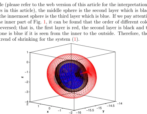
3-D phase portrait is shown in Fig.1. There are three layers in this diagram. The outermost sphere is the first layer which is red on the web version of this
article (please refer to the web version of this article for the interpretation of colors in this article), the middle sphere is the second layer which is black, and the innermost sphere is the third layer which is blue. If we pay attention to the inner part of Fig.1, it can be found that the order of different colors are reversed; that is, the first layer is red, the second layer is black and the last one is blue if it is seen from the inner to the outside. Therefore, there is a trend of shrinking for the system (1).
−2 −1 0 1 2 −16 −15.5 −15 −14.5 −14 −4 −3 −2 −1 0 1 y x z
Fig. 1. A typical 3-layer “chaotic attractor” of the system witha1=−4.1,a2= 1.2, a3= 13.45,c1= 2.76,c2= 0.6,c3= 13.13andd= 1.6.
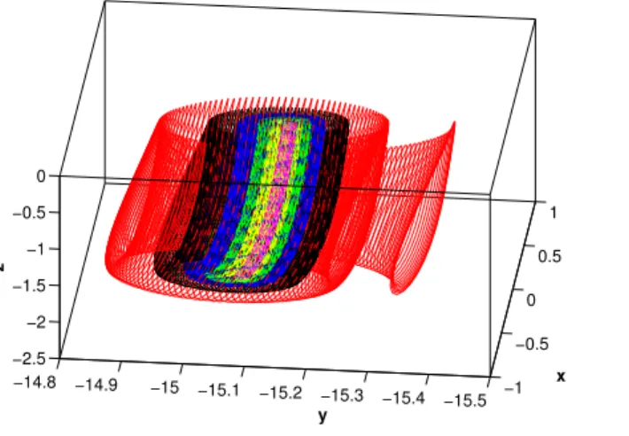
What will happen if the simulation time is longer than 130 s? If the simulation time is sett= 380s, the phase diagram is shown in Fig.2where the phase diagram is not drawn from 0 s to 130 s. As can be seen from Fig.2, there are six layers. The colors of them are red, black, blue, green, yellow and magenta, respectively, from the outside to the inner one which means there is a trend of shrinking. According to the analysis, the diagram maybe shrink to a curve if the simulation time is long enough. This hypothesis is easy to be proved using the portrait diagram without transient states if the simulation time is set to be longer. If simulation time t = 1500 s, the solutions of system (1) will reach a limit cycle as shown in Fig.3.
These numerical evidences reveal that system (1) does not show chaotic dynamics, which is different from the result in [5], when with a1 = −4.1,
a2 = 1.2,a3= 13.45,c1 = 2.76,c2 = 0.6,c3= 13.13and d= 1.6.
Lyapunov exponents are another important numerical method to prove whether one nonlinear system is chaotic or not. If the Wolf algorithm [18] is used to calculate the Lyapunov exponents, the simulation time is set as 15000 s and the sampling time-step is 0.0001 s, the Lyapunov exponents of system (1) are λ1 = 0, λ2 = −0.0138 and λ3 = −0.0141, which mean
the final states are periodic orbit, when a1 = −4.1, a2 = 1.2, a3 = 13.45,
Zenghui Wang, Yanxia Sun, Shijian Cang −1 −0.5 0 0.5 1 −15.5 −15.4 −15.3 −15.2 −15.1 −15 −14.9 −14.8 −2.5 −2 −1.5 −1 −0.5 0 x y z
Fig. 2. Phase portrait of the system (1) with a1 =−4.1, a2 = 1.2, a3 = 13.45, c1= 2.76, c2= 0.6, c3= 13.13andd= 1.6if the simulation time is from 130 s to 380 s. −1 −0.5 0 0.5 −15.14 −15.12 −15.1 −15.08 −15.06 −15.04 −2.5 −2 −1.5 −1 −0.5 x y z
Fig. 3. Final states of the system (1) with a1 = −4.1, a2 = 1.2, a3 = 13.45, c1= 2.76,c2= 0.6,c3= 13.13andd= 1.6.
the similar results can be obtained which are different from the results in [5] such as some phase portraits in Fig. 2 of Ref. [5]. The numerical evidences show that it is not reliable to construct chaotic system only based on the Šhilnikov criterion. Other numerical methods should also be used together to prove the nonlinear systems show chaotic dynamics.
There is a logical question about how to construct a chaotic attractor which can show sphere shape. According to the analysis of phase portrait of system (1), breaking the trend of shrinking and keeping the chaotic dynamics can make the system (1) show sphere shape. Using this idea, a new system is proposed in the following section.
3. A 3-D spherical chaotic attractor
A simple method to break the trend of shrinking is adding small pertur-bance to the first or the third equation of system (1). Here, a sign function is added to the first equation of system (1), that is
˙ x = a1x−a2y+a3z+ 2sign(sin y), ˙ y = −dxz+b , ˙ z = c1xy+c2yz+c3z+c . (2)
Heresign(·) is the sign function. The sign functions have been used in [19]
to produce sphere chaotic attractors. However, the spherical attractors were proposed in the polar coordinate and then they were transferred to the space
(x, y, z). Moreover, two sign functions were used in [19] and one sign function is used in the proposed system. The analytical methods of [19] cannot be directly used in the proposed system as the spherical attractors of [19] were proposed and analyzed using the polar coordinate.
When a1 =−4.1,a2 = 1.2,a3= 13.45,c1= 2.76,c2= 0.6,c3= 13.13,
b= 0.161, c= 3.5031, d= 1.6, we can get one equilibrium for system (2), that is, (xe, ye, ze) = (0.7217,−2.5698,0.1394).The Jacobian matrix
corre-sponding to(xe, ye, ze)is X = a1 −a2 a3 −dze 0 −dxe c1ye c1xe+c2ze c2ye+c3 . (3)
It can be found that the Jacobian system evaluated at the only one equi-librium point has three roots, one negative real root and a conjugate pair of complex roots with positive real parts when a1 = −4.1, a2 = 1.2, a3 =
13.45, c1 = 2.76, c2 = 0.6, c3 = 13.13, b = 0.161, c = 3.5031 and d = 1.6,
which means it is possible that there is a homoclinic orbit. It would be better to use other numerical methods to prove this nonlinear system shows chaotic dynamics as it is difficult to find the sensitive homoclinic orbit.
When a1 =−4.1,a2 = 1.2,a3 = 13.45, c1 = 2.76,c2 = 0.6,c3 = 13.13,
b = 0.161, c = 3.5031, d = 1.6, the initial condition is (0.1,0.1,0.1), the simulation time is 1500 s and only the data of the last 100 s is used, the 3-D phase portrait is shown in Fig.4. As can be seen from Fig.4, this attractor shows sphere shape. However, the sign function is not a smooth function.
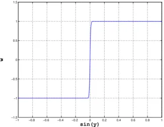
If the sign function is replaced by a hyperbolic tangent function, this system will be a smooth system and will show the similar dynamics. Fig.5 shows the phase portrait ofw=w(sin y) = 1−e−200 siny/1+e−200 sinywhen −1≤sin y≤y. As can be seen from Fig.5,wfunction can closely approach the sign function. In this paper, the 64-bit double-precision floating-point
Zenghui Wang, Yanxia Sun, Shijian Cang −2 −1 0 1 2 −17 −16 −15 −14 −13 −6 −4 −2 0 2 x y z
Fig. 4. Phase portrait of the system (2) with a1 =−4.1, a2 = 1.2, a3 = 13.45, c1= 2.76,c2= 0.6,c3= 13.13, b= 0.161,c= 3.5031andd= 1.6.
number is used in Matlab and Visual C++ to do numerical computation. It should be noted that 1−e−200 siny/1 +e−200 siny will be 1 (or−1) when
sin y approaches 1 (or −1). For example, the numerator is 1−e−200 when
sin y is 1. However, e−200 is approximately equal to 10−85 and the whole numerator is 1−10−85, that is 0.99999. . . (85 times “9” followed by “0”). The mantysa must contain 85 decimal digits to be distinguished from the value one. The similar is true for the denominator. Hence, the effect ofsiny terms will not be visible and w function is equal to the sign function when
sin yapproaches 1 (or −1), as the mantysa accuracy of the compiler is only 16 decimal digits (53 bits).
−1 −0.8 −0.6 −0.4 −0.2 0 0.2 0.4 0.6 0.8 1 −1.5 −1 −0.5 0 0.5 1 1.5 sin(y) w
To analyze the complicated dynamics of the new system, a linear term exis added to the second equation of the system (2). Then, the new system is proposed as ˙ x = a1x−a2y+a3z+ 2 1−e−200 siny 1 +e−200 siny , ˙ y = −dxz+b+ex, ˙ z = c1xy+c2yz+c3z+c . (4) When a1 =−4.1,a2 = 1.2,a3 = 13.45, c1 = 2.76,c2 = 0.6,c3 = 13.13,
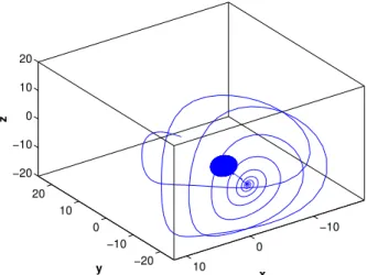
b = 0.161, c = 3.5031, d = 1.6; the initial condition is (0.1,0.1,0.1), the simulation time is 600 s, the 3-D phase portrait is shown in Fig. 6. In this paper, the initial conditions are(0.1,0.1,0.1)if they are not specifically given. With these parameters, system (4) is chaotic and the corresponding Lyapunov exponents are(0.041,0,−0.117). As can be seen from Fig.6, the orbit starts from the initial conditions and then reaches the sphere chaotic attractor. −10 0 10 −20 −10 0 10 20 −20 −10 0 10 20 x y z
Fig. 6. Sphere chaotic attractor with the transient part, witha1=−4.1,a2= 1.2, a3 = 13.45, c1 = 2.76, c2 = 0.6, c3 = 13.13, b = 0.161, c = 3.5031, d= 1.6 and e= 0.
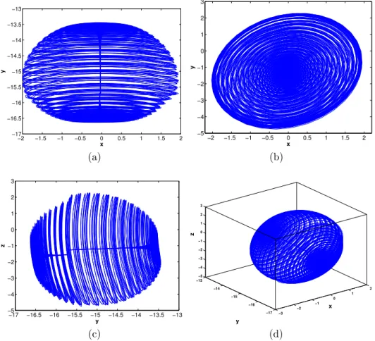
When discarding the transient part of the phase diagram, it would be clear to find the sphere shape of the chaotic attractor of the system (4). The projections of phase portrait on x–y, x–z, and y–z plane are shown in Fig. 7(a), Fig. 7(b) and Fig. 7(c), respectively, and the 3-D chaotic attractor is shown in Fig.7(d). If the simulation time is long enough, the chaotic attractor will form a close sphere.
Zenghui Wang, Yanxia Sun, Shijian Cang −2 −1.5 −1 −0.5 0 0.5 1 1.5 2 −17 −16.5 −16 −15.5 −15 −14.5 −14 −13.5 −13 x y −2 −1.5 −1 −0.5 0 0.5 1 1.5 2 −5 −4 −3 −2 −1 0 1 2 3 x y (a) (b) −17 −16.5 −16 −15.5 −15 −14.5 −14 −13.5 −13 −5 −4 −3 −2 −1 0 1 2 3 y z −3 −2 −1 0 1 2 −17 −16 −15 −14 −13 −5 −4 −3 −2 −1 0 1 2 3 x y z (c) (d)
Fig. 7. Sphere chaotic attractor without the transient part, with a1=−4.1, a2=
1.2, a3 = 13.45, c1 = 2.76, c2 = 0.6, c3 = 13.13, b = 0.161, c = 3.5031, d= 1.6
and e = 0. (a) Projection on the x–y plane; (b) Projection on the x–z plane; (c) Projection on they–z plane; (d) 3-D view in thex–y–z space.
3.1. Bifurcation analysis with respect to parameter e
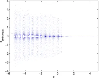
Fig.8 shows the bifurcation diagram of the state variable x. In Fig. 8, the variable parameter ise, varied from −6 to 5. Generally, there exist two divisions in the parameter region of e, that is, sink and chaotic regions.
Fig.9shows the Lyapunov exponent spectra, which directly corresponds to the bifurcation diagram shown in Fig.8. The Lyapunov exponent spectra also prove that there exist two divisions in the parameter region of e, that is, sink and chaotic regions. It can be observed that the system is chaotic in the region of−5.6≤e≤0.3.
−6 −4 −2 0 2 4 −4 −3 −2 −1 0 1 2 3 4 e x (min/max)
Fig. 8. The bifurcation diagram of the system (4) with respect to e, and with
a1 = −4.1, a2 = 1.2, a3 = 13.45, c1 = 2.76, c2 = 0.6, c3 = 13.13, b = 0.161, c= 3.5031, andd= 1.6. −6 −4 −2 0 2 4 −0.8 −0.6 −0.4 −0.2 0 0.2 0.4 e Lyapunov Exponent
Fig. 9. The Lyapunov exponent spectra of the system (4) with respect to e, and witha1 =−4.1, a2= 1.2, a3= 13.45, c1 = 2.76, c2 = 0.6, c3 = 13.13, b = 0.161, c= 3.5031andd= 1.6.
As can be seen from Fig. 8 and Fig. 9, there is no region which shows cycle whena1=−4.1,a2= 1.2,a3 = 13.45,c1 = 2.76,c2 = 0.6,c3= 13.13,
b= 0.161, c = 3.5031 and d = 1.6. What will happen if other parameters are changed?
Zenghui Wang, Yanxia Sun, Shijian Cang
If the parametere is fixed as 0 and the parameter a2 is varied, Fig. 10
shows the bifurcation diagram of the state variablex with respect to a2.
−3 −2 −1 0 1 2 3 −2.5 −2 −1.5 −1 −0.5 0 0.5 1 1.5 2 2.5 a2 x(min/max)
Fig. 10. The bifurcation diagram of the system (4) with respect to a2, and with a1 = −4.1, a3 = 13.45, c1 = 2.76, c2 = 0.6, c3 = 13.13, b = 0.161, c = 3.5031, d= 1.6 ande= 0.
Fig.11shows the Lyapunov exponent spectra, which directly corresponds to the bifurcation diagram shown in Fig. 10.
−3 −2 −1 0 1 2 3 −4 −3.5 −3 −2.5 −2 −1.5 −1 −0.5 0 0.5 1 a 2 Lyapunov Exponent
Fig. 11. The Lyapunov exponent spectra of the system (4) with respect toa2, and witha1=−4.1,a3= 13.45,c1= 2.76,c2= 0.6,c3= 13.13,b= 0.161, c= 3.5031, d= 1.6 ande= 0.
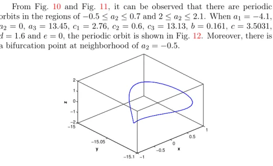
From Fig. 10 and Fig. 11, it can be observed that there are periodic orbits in the regions of−0.5≤a2 ≤0.7and2≤a2≤2.1. Whena1 =−4.1,
a2 = 0, a3 = 13.45, c1 = 2.76, c2 = 0.6, c3 = 13.13, b= 0.161, c= 3.5031,
d= 1.6ande= 0, the periodic orbit is shown in Fig.12. Moreover, there is a bifurcation point at neighborhood ofa2=−0.5.
−1 −0.5 0 0.5 1 −15.1 −15.05 −15 −2 −1 0 1 2 x y z
Fig. 12. Periodic orbit of system (4) whena1=−4.1,a2= 0,a3= 13.45,c1= 2.76, c2= 0.6,c3= 13.13,b= 0.161,c= 3.5031,d= 1.6 ande= 0.
3.2. Poincaré section of the spherical chaotic attractor
To show graphically what happens, the Poincaré section is used. When a1 =−4.1, a2 = 1.2,a3= 13.45, c1 = 2.76,c2 = 0.6,c3 = 13.13,b= 0.161,
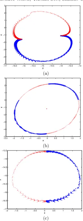
c= 3.5031, d= 1.6 and e= 0, one may take x = 0, y =−15 and z = 0 as crossing planes, respectively. Fig.13shows the Poincaré mapping on several sections with circle shape of the attractors visualized. Moreover, there is finite thickness for these circles. Symbols “·” (red on-line) are determined by positively crossing Poincaré sections and symbols “+” (blue) are deter-mined by negatively crossing Poincaré sections. As can be seen from Fig.13, the shape of the attractor of system (4) is a spherical surface and there is connection between two poles that is shown by a point (red) in the center of Fig. 13(b). If using different value of the system parameters, the point of Fig. 13(b) might be a circle and the chaotic attractor would be “fractal torus”. The “fractal torus” attractor is very interesting because it exhibits a structure entirely different from attractors such as the Rössler and Lorenz attractors. Rather than consisting of separate, “flat” sheets, this kind of at-tractor typically consists of a “slow” and a “fast” manifold, shaped like a fat doughnut, with the slow dynamics being confined to a very skinny tube on the inside of the doughnut and the fast, oscillatory dynamics taking place on the outside of the doughnut. Numerical experiments with Poincare sec-tion allow us to conclude that the system (7) shows a 3-D spherical chaotic attractor, which is also a “fractal torus”.
Zenghui Wang, Yanxia Sun, Shijian Cang −17 −16.5 −16 −15.5 −15 −14.5 −14 −13.5 −13 −5 −4 −3 −2 −1 0 1 2 3 y z (a) −2.5 −2 −1.5 −1 −0.5 0 0.5 1 1.5 2 −5 −4 −3 −2 −1 0 1 2 3 x z (b) −2 −1.5 −1 −0.5 0 0.5 1 1.5 2 −17 −16.5 −16 −15.5 −15 −14.5 −14 −13.5 x y (c)
Fig. 13. Four-wing chaotic attractor Poincaré sections: witha1 =−4.1, a2= 1.2, a3 = 13.45, c1 = 2.76, c2 = 0.6, c3 = 13.13, b = 0.161, c = 3.5031, d = 1.6 and e= 0. (a) Poincaré map on the crossing-sectionx= 0; (b) Poincaré map on the crossing-sectiony=−15; (c) Poincaré map on the crossing-sectionz= 0.
4. Conclusion
A 3-layer sphere chaotic attractor was analyzed. It was found that it is limit a cycle instead of chaotic attractor and that is caused by the simu-lation time. Moreover, it is shown that the exact homoclinic orbits should also be found when we construct a chaotic system based on the Šhilnikov criterion. Otherwise, other numerical methods should be used together to prove a nonlinear system shows chaotic dynamics. With the analysis, a chaotic system with the real sphere shape was proposed. This system was investigated through numerical simulations and analyses, which showed the proposed system is a real smooth sphere chaotic system.
REFERENCES
[1] M. Bharathwaj,Int. J. Bifur. Chaos 20, 1335 (2010). [2] R.K. Sheline, P. Alexa,Acta Phys. Pol. B 39, 711 (2008). [3] C.Y. Ho, B.W. Ling,Int. J. Bifur. Chaos 20, 1279 (2010). [4] A.Z. Gorski, T. Srokowski,Acta Phys. Pol. B 37, 9 (2006). [5] T.S. Zhou, G. Chen,Int. J. Bifur. Chaos 14, 1795 (2004).
[6] G. Chen, in Chaos Control: Theory and Applications, eds. G. Chen, X. Yu, Springer-Verlag, Berlin 2003, pp. 159–178.
[7] G. Chen, T. Ueta, Int. J. Bifur. Chaos 9, 1465 (1999). [8] T.S. Zhou, G. Chen,Int. J. Bifur. Chaos 16, 2459 (2006).
[9] M.E. Yalcin, J.A.K. Suykens, J. Vandewalle, S. Ozoguz,Int. J. Bifur. Chaos
12, 23 (2002).
[10] L.O. Chua, M. Komuro, T. Matsumoto,IEEE Trans. Circuits Systems-I 33, 1072 (1986).
[11] Y.G. Zheng, G. Chen,Int. J. Bifur. Chaos 14, 279 (2004). [12] E.N. Lorenz,J. Atmos. Sci. 20, 130 (1963).
[13] O.E. Rössler,Phys. Lett. A 57, 397 (1976). [14] J.C. Sprott,Phys. Rev. E 50, 647 (1994).
[15] T.S. Zhou, G. Chen, Q.G. Yang,Chaos Solitons Fractals 19, 985 (2004). [16] Z. Wang, G. Qi, B.J. van Wyk, M.A. van Wyk,Int. J. Bifur. Chaos19, 3841
(2009).
[17] Y. Sun, G. Qi, Z. Wang, B.J. van Wyk,Acta Phys. Pol. B 41, 767 (2010). [18] A. Wolf, J.B. Swift, H.L. Swinney, J.A. Vastano,Physica D 16, 285 (1985). [19] Q. Chen, Y. Hong, G. Chen,Physica A 371, 293 (2006).