Time Series Prediction Using Radial Basis Function Neural Network

ISSN: 2088-8708  765

Time Series Prediction Using Radial Basis Function Neural

Network

Haviluddin*, Imam Tahyudin**

* Dept. of Computer Science, Faculty of Mathematic and Natural Science, Mulawarman University, Indonesia ** Dept. of Information System, STMIK AMIKOM Purwokerto, Indonesia

Article Info ABSTRACT

Article history: Received Dec 18, 2014 Revised Apr 23, 2015 Accepted May 16, 2015

This paper presents an approach for predicting daily network traffic using artificial neural networks (ANN), namely radial basis function neural network (RBFNN) method. The data is gained from 21-24 June 2013 (192 samples series data) in ICT Unit of Mulawarman University, East Kalimantan, Indonesia. The results of measurement are using statistical analysis, e.g. sum of square error (SSE), mean of square error (MSE), mean of absolute percentage error (MAPE), and mean of absolute deviation (MAD). The results show that values are the same, with different goals that have been set are 0.001, 0.002, and 0.003, and spread 200. The smallest MSE value indicates a good method for accuracy. Therefore, the RBFNN model illustrates the proposed best model to predict daily network traffic.

Keyword: MAD MAPE MSE Network traffic RBFNN

SSE Copyright © 2015 Institute of Advanced Engineering and Science. All rights reserved. Corresponding Author:

Haviluddin,

Dept. of Computer Science,

Faculty of Mathematics and Natural Science,

Mulawarman University, East Kalimantan, Indonesia. Email: [email protected]

1. INTRODUCTION

The management of traffic quota is an important part, especially for the organizations that use information technology. Subsequently, for the leadership, management traffic quota will help in making decisions that will benefit the efficiency and effective for organizations including universities.

The predicting activities are a part of organization management. Subsequently, the daily network traffic prediction is also a process of analyzing and determining the quota of bandwidth in a network in the future, in which a technical analysis approach usage data traffic. Furthermore, the predicting techniques used in the literature can be classified into two categories: statistical and soft-computing models. The statistical models includes simple regression linear (SRL), exponential smoothing, the autoregressive moving average (ARMA), autoregressive integrated moving average (ARIMA) and generalized autoregressive conditional heteroskedasticity (GARCH) models. Nevertheless, these models are focused around the supposition that the several of time series data linearly correlate and provide poor prediction performance [1-5].

Meanwhile, the daily network traffic data are nonlinear and non-stationary in nature. To overcome this limitation, the second model is soft-computing methods have been suggested. Furthermore, modeling using the artificial neural network (ANN) model can provide better analytical results, and it is effective for forecasting, in which this method is able to work well on the non-linear time-series data [3, 6-8].

Therefore, this paper will study one of the ANN models, namely the Radial Basis Function Neural Network (RBFNN), in order to address the issue of network traffic time series data that has non-linear characteristics. This paper consists of four sections. Introduction section is the motivation to do the writing of

the article. Next, the methodology is describes of model. Third section is the analysis and discussion results, and finally conclusion section is research summaries.

2. RESEARCH METHOD

The RBFNN is the abbreviation of radial basis function neural network which is based on the function approximation theory or supervised and unsupervised manner were used together. Subsequently, it has a unique training algorithm called hybrid method that emerged as a variant of NN in late 80’s. This model is a kind of feed-forward neural network (FFNN) in which includes an input layer, a hidden layer, and an output layer [9, 10] as seen in Figure 1.

Figure 1. RBF neural network structure [11]

In general, RBFNN process the first phase is unsupervised learning between input layer and hidden layer that non-linear radial-based activation functions, commonly Gaussian function. Second phase is supervised learning between hidden layer and output layer with a linear.

‖ 1 ‖ 1

where

‖ 1 ‖ is the Euclidean distance, c is the center of Gaussian function 1, 2, … , , … , is the qth input data.

Hence, in this this study the architecture of RBFNN as shown in Figure 2, and the equation is

.

where:

Y = output value; φ = hidden value; W = weights (0-1)

The algorithm of RBFNN to analyze within time series data characteristics is: 1. Initialization of the network.

2. Determining the input signal to hidden layer, and find is a distance data to where , 1,2, … ,

3. Find 1 is a result activation from distance data multiply bias.

1 ∗

4. Find weight and bias layers, 2 and 2 , in each 1,2, … , Determining training samples and test samples

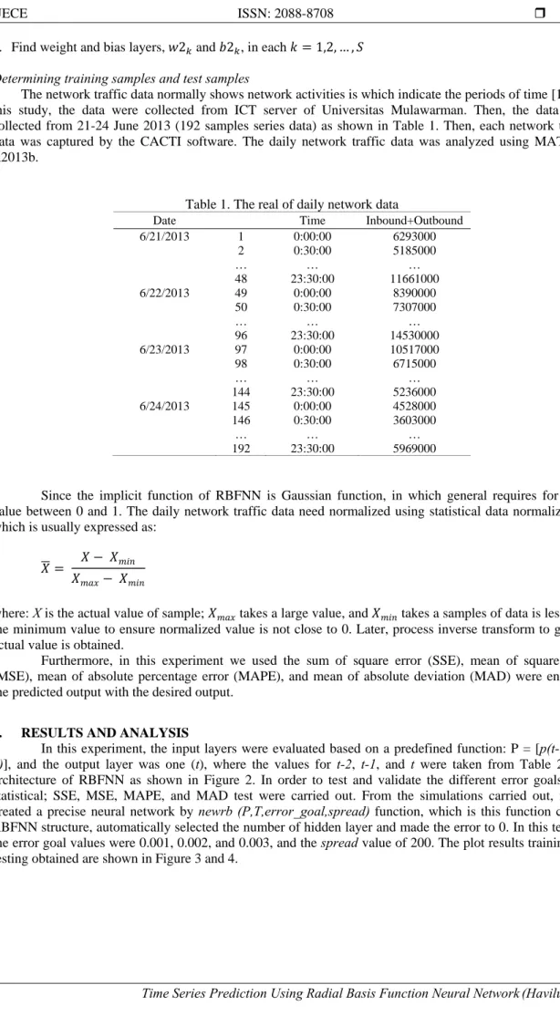
The network traffic data normally shows network activities is which indicate the periods of time [12]. In this study, the data were collected from ICT server of Universitas Mulawarman. Then, the data were collected from 21-24 June 2013 (192 samples series data) as shown in Table 1. Then, each network traffic data was captured by the CACTI software. The daily network traffic data was analyzed using MATLAB R2013b.

Table 1. The real of daily network data

Date Time Inbound+Outbound 6/21/2013 1 0:00:00 6293000 2 0:30:00 5185000 … … … 48 23:30:00 11661000 6/22/2013 49 0:00:00 8390000 50 0:30:00 7307000 … … … 96 23:30:00 14530000 6/23/2013 97 0:00:00 10517000 98 0:30:00 6715000 … … … 144 23:30:00 5236000 6/24/2013 145 0:00:00 4528000 146 0:30:00 3603000 … … … 192 23:30:00 5969000

Since the implicit function of RBFNN is Gaussian function, in which general requires for input value between 0 and 1. The daily network traffic data need normalized using statistical data normalization, which is usually expressed as:

where: X is the actual value of sample; takes a large value, and takes a samples of data is less than the minimum value to ensure normalized value is not close to 0. Later, process inverse transform to get the actual value is obtained.

Furthermore, in this experiment we used the sum of square error (SSE), mean of square error (MSE), mean of absolute percentage error (MAPE), and mean of absolute deviation (MAD) were engaged the predicted output with the desired output.

3. RESULTS AND ANALYSIS

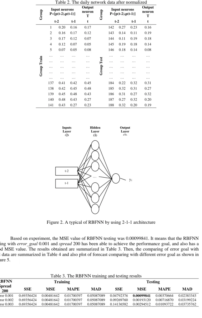
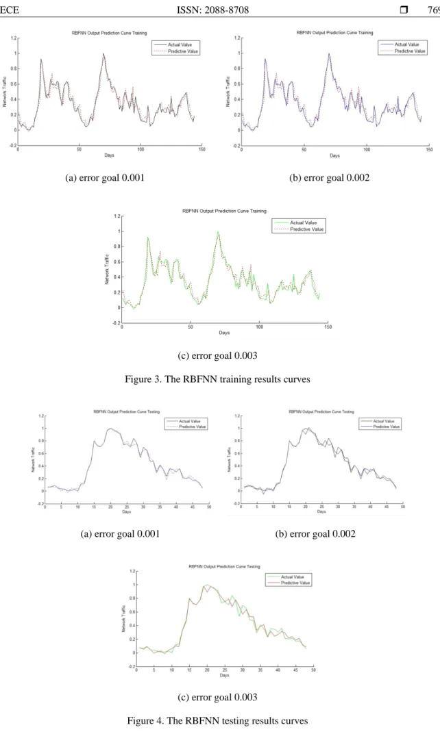
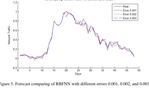
In this experiment, the input layers were evaluated based on a predefined function: P = [ p(t-2),p(t-1)], and the output layer was one (t), where the values for t-2, t-1, and t were taken from Table 2. The architecture of RBFNN as shown in Figure 2. In order to test and validate the different error goals, four statistical; SSE, MSE, MAPE, and MAD test were carried out. From the simulations carried out, it was created a precise neural network by newrb (P,T,error_goal,spread) function, which is this function creates RBFNN structure, automatically selected the number of hidden layer and made the error to 0. In this test, for the error goal values were 0.001, 0.002, and 0.003, and the spread value of 200. The plot results training and testing obtained are shown in Figure 3 and 4.

Table 2. The daily network data after normalized Gro u p Input neurons P=[p(t-2),p(t-1)] Output neuron T Gro u p Input neurons P=[p(t-2),p(t-1)] Output neuron T t-2 t-1 t t-2 t-1 t Group Train 1 0.20 0.16 0.17 Group Tes t 142 0.27 0.23 0.16 2 0.16 0.17 0.12 143 0.14 0.11 0.19 3 0.17 0.12 0.07 144 0.11 0.19 0.18 4 0.12 0.07 0.05 145 0.19 0.18 0.14 5 0.07 0.05 0.08 146 0.18 0.14 0.08 … … … … … … … … … … … … … … … … … … … … … … … … … … … … … … … … … … … … … … … … 137 0.41 0.42 0.45 184 0.22 0.32 0.31 138 0.42 0.45 0.48 185 0.32 0.31 0.27 139 0.45 0.48 0.43 186 0.31 0.27 0.32 140 0.48 0.43 0.27 187 0.27 0.32 0.20 141 0.43 0.27 0.23 188 0.32 0.20 0.19

Figure 2. A typical of RBFNN by using 2-1-1 architecture

Based on experiment, the MSE value of RBFNN testing was 0.00099841. It means that the RBFNN setting with error_goal 0.001 and spread 200 has been able to achieve the performance goal, and also has a good MSE value. The results obtained are summarized in Table 3. Then, the comparing of error goal with real data are summarized in Table 4 and also plot of forecast comparing with different error goal as shown in Figure 5.

Table 3. The RBFNN training and testing results

RBFNN Spread

200

Training Testing

SSE MSE MAPE MAD SSE MSE MAPE MAD

Error 0.001 0.69356424 0.00481642 0.01700397 0.05087089 0.04792376 0.00099841 0.00370664 0.02383343 Error 0.002 0.69356424 0.00481642 0.01700397 0.05087089 0.09269760 0.00193120 0.00716870 0.03199224 Error 0.003 0.69356424 0.00481642 0.01700397 0.05087089 0.14136582 0.00294512 0.01093722 0.03735762 t-2 Inputs Layer (2) Hidden Layer (1) Output Layer (1) … t-1 y1

(a) error goal 0.001 (b) error goal 0.002

(c) error goal 0.003

Figure 3. The RBFNN training results curves

(a) error goal 0.001 (b) error goal 0.002

Figure 5. Forecast comparing of RBFNN with different errors 0.001, 0.002, and 0.003

Table 4. Comparing RBFNN with error goal 0.001, 0.002, and 0.003

Real Error Goal Real Error Goal

0.001 0.002 0.003 0.001 0.002 0.003 0.06648 0.00576 0.02339 -0.01052 0.75081 -0.04932 0.02717 0.00237 0.06821 -0.00802 -0.02441 0.01375 0.70386 -0.01774 -0.10069 -0.09002 0.09296 0.02926 0.02474 0.00339 0.84143 0.10252 0.11271 0.16598 0.04712 -0.02022 -0.01998 0.00321 0.76235 0.01517 0.01138 -0.01479 0.03522 0.03830 0.02005 0.03814 0.53622 -0.03948 -0.08967 -0.14309 0.02830 -0.01737 -0.03236 0.00922 0.69768 0.04575 0.10624 0.13175 0.00881 0.03641 0.05861 -0.01996 0.65155 -0.00928 -0.01080 0.01840 0.01293 -0.03549 -0.03112 0.02804 0.48350 -0.04717 -0.04191 -0.04722 0.02628 -0.00942 -0.00502 -0.01180 0.47197 -0.01007 -0.05560 -0.06083 0.00000 -0.03957 -0.02515 -0.06509 0.29280 -0.02275 -0.03760 -0.04238 0.11825 0.02740 0.02379 0.01762 0.41143 -0.01146 0.00263 0.02369 0.13118 0.02091 0.00641 0.03629 0.35088 0.00024 -0.00034 -0.06424 0.32411 -0.00742 -0.00781 0.00047 0.23926 0.06008 0.05066 0.00546 0.45097 -0.00468 0.00031 -0.02004 0.35747 0.00394 0.01209 0.04141 0.80065 0.00281 0.00073 0.00875 0.34882 0.07321 0.08476 0.10722 0.72075 -0.00024 -0.00223 -0.00458 0.30475 -0.04591 -0.04076 0.03432 0.70963 0.00052 0.00388 0.00295 0.35953 0.00986 0.02875 0.04318 0.77470 -0.00014 -0.00278 -0.00464 0.21002 -0.03086 -0.05778 -0.07835 0.96993 -0.00063 0.00352 -0.00526 0.20091 0.00888 0.01178 -0.01676 1.00000 -0.00723 0.09571 0.10845 0.21426 -0.03785 -0.03213 -0.02329 0.97941 0.02999 -0.03414 0.00787 0.16862 -0.04646 -0.02968 -0.01739 0.94151 -0.02249 -0.00014 -0.00534 0.17764 0.01979 -0.02188 -0.03695 0.91927 0.02723 0.03738 0.03110 0.12369 -0.01743 -0.00511 0.01358 0.74010 -0.01334 -0.05879 -0.07801 0.05445 0.01395 0.02108 -0.03606 4. CONCLUSION

In this paper, the analysis using RBFNN technique to achieve the model of daily network traffic activities have been conducted in the ICT Unit, Universitas Mulawarman. According to Figure 3 and 4, the results of RBFNN training shows that for error goal value is 0.001 then SSE value is 0.69356424, MSE value is 0.00481642, MAPE value is 0.01700397, and MAD value is 0.05087089. Afterward, the values of the RBFNN testing are SSE value is 0.04792376, MSE value is 0.00099841, MAPE value is 0.00370664, and MAD value is 0.02383343. Based on results, RBFNN with parameter error goal 0.001 and spread 200 has been able a good MSE value. In other words, the RBFNN are considered closer to the actual value.

According to indicator test result of data is the smallest error value, where value indicating an error testing is the best model [11]. Therefore, the determination of the best model is determined by selecting the smallest value of testing error. In other words, the RBFNN model with different error goal values illustrates the proposed best model to predict daily network traffic activities. Therefore, one of the planned future works is to combine the RBFNN method with a genetic algorithm (GA) in order to optimize the prediction accuracy.

ACKNOWLEDGEMENTS

This study has been completed thanks to the help and support from various parties that cannot be mentioned one by one. Especially thank you to our family, children and wife. Researchers say a big thank you to family of Mulawarman University and STMIK AMIKOM Purwokerto who has given support to complete this study. Hopefully this research can be useful.

REFERENCES

[1] Haviluddin, and R. Alfred, “Forecasting Network Activities Using ARIMA Method”, Journal of Advances in Computer Networks, vol. 2, no. 3, September 2014, pp. 173-179, 2014.

[2] B. Majhi, M. Rout, and V. Baghel, “On the development and performance evaluation of a multiobjective GA-based RBF adaptive model for the prediction of stock indices”, Journal of King Saud University-Computer and Information Sciences, no. 2014, 2014.

[3] Y. Birdi, T. Aurora, and P. Arora, “Study of Artificial Neural Networks and Neural Implants”, International Journal on Recent and Innovation Trends in Computing and Communication, vol. 1, no. 4, 2013.

[4] U. Yolcu, E. Egrioglu, and C.H. Aladag, “A new linear & nonlinear artificial neural network model for time series forecasting”, Decision Support Systems, vol. 54, no. 2013, pp. 1340–1347, 2013.

[5] L. Abdullah, “ARIMA Model for Gold Bullion Coin Selling Prices Forecasting”, International Journal of Advances in Applied Sciences (IJAAS), vol. 1, no. 4, December 2012, pp. 153-158, 2012.

[6] O. Claveria, and S. Torra, “Forecasting tourism demand to Catalonia: Neural networks vs. time series models”, Economic Modelling, vol. 36, no. 2014, pp. 220–228, 2014.

[7] J.Z. Wang, J.J. Wang, Z.G. Zhang et al., “Forecasting stock indices with back propagation neural network”, Expert Systems with Applications, vol. 38, no. 2011, pp. 14346–14355, 2011.

[8] G. Chen, K. Fu, Z. Liang et al., “The genetic algorithm based back propagation neural network for MMP prediction in CO2-EOR process”, Fuel, vol. 126, no. 2014, pp. 202–212, 2014.

[9] W. Jia, D. Zhao, T. Shen et al., “A New Optimized GA-RBF Neural Network Algorithm”, Computational Intelligence and Neuroscience, no. 2014, pp. 1-6, 2014.

[10]Y. Zhijun, “RBF Neural Networks Optimization Algorithm and Application on Tax Forecasting”, TELKOMNIKA, vol. 11, no. 7, July 2013, pp. 3491 - 3497, 2013.

[11]J. Wu-Yu, and J. Yu, “Rainfall time series forecasting based on Modular RBF Neural Network model coupled with SSA and PLS”, Journal of Theoretical and Applied Computer Science, vol. 6, no. 2, pp. 3-12, 2012.

[12]Haviluddin, and R. Alfred, “Comparison of ANN Back Propagation Techniques in Modelling Network Traffic Activities”. pp. 224-231.

BIOGRAPHIES OF AUTHORS

Haviluddin was born in Loa Tebu, East Kalimantan, Indonesia. He graduated from STMIK WCD Samarinda in the field of Management Information, and he completed a Master at Universitas Gadjah Mada, Yogyakarta in the field of Computer Science. He is also a Lecturer in the Department of Computer Science, Faculty of Mathematics and Natural Science, Universitas Mulawarman, East Kalimantan, Indonesia. Currently, he is pursuing his PhD in the field of Computer Science at the Faculty of Computing and Informatics, Universiti Malaysia Sabah, Malaysia. He is a member of the Institute of Electrical and Electronic Engineers (IEEE), Institute of Advanced Engineering and Science (IAES), and Indonesian Computer, Electronics, Instrumentation Support Society (IndoCEISS), and Association of Computing and Informatics Institutions Indonesia (APTIKOM) societies.

Imam Tahyudin was born in Indramayu, West Java, Indonesia. He graduated from Jenderal Soedirman University, Purwokerto in 2006 in the field of Mathematics, and he completed a Master at Jenderal Soedirman University in 2010 in the field of Management. Then, he graduated a master degree at STMIK AMIKOM Yogyakarta in 2013 in field of Information Technology. He is also a Lecturer in STMIK AMIKOM Purwokerto, Central Java, Indonesia. Currently, he is a Head of LPPM of STMIK AMIKOM Purwokerto. He is a member of Institute of Advanced Engineering and Science (IAES), Association of Computing and Informatics Institutions Indonesia (APTIKOM), Indonesian Computer, Electronics, Instrumentation Support Society (IndoCEISS), Association of Information System (AIS) and Association of Information System for Indonesia (AISINDO).