Fraser L. Greenroyd
1,2, Rebecca Hayward
2, Andrew Price
1, Peter Demian
1and Shrikant Sharma
2 1Centre for Innovative and Collaborative Construction Engineering, School of Civil and Building Engineering,Loughborough University, Loughborouogh, U.K.
2BuroHappold Engineering, Bath, U.K.
Keywords: Hospital Operations, Patient Scheduling, Discrete-event Simulation, Healthcare Delivery, Outpatient Operations.
Abstract: As the National Health Service (NHS) of England continues to face tighter cost saving and utilisation government set targets, finding the optimum between costs, patient waiting times, utilisation of resources, and user satisfaction is increasingly challenging. Patient scheduling is a subject which has been extensively covered in the literature, with many previous studies offering solutions to optimise the patient schedule for a given metric. However, few analyse a large range of metrics pertinent to the NHS. The tool presented in this paper provides a discrete-event simulation tool for analysing a range of patient schedules across nine metrics, including: patient waiting, clinic room utilisation, waiting room utilisation, staff hub utilisation, clinician utilisation, patient facing time, clinic over-run, post-clinic waiting, and post-clinic patients still being examined. This allows clinic managers to analyse a number of scheduling solutions to find the optimum schedule for their department by comparing the metrics and selecting their preferred schedule. Also provided is an analysis of the impact of variations in appointment durations and their impact on how a simulation tool provides results. This analysis highlights the need for multiple simulation runs to reduce the impact of non-representative results from the final schedule analysis.
1
INTRODUCTION
The National Health Service (NHS) of England, despite being viewed as one of the best health systems in the Western world (Davis et al., 2014), is facing some of the toughest challenges since its inception in 1948 (NHS England, 2013). Since 2009 these challenges have been focussed heavily on cost efficiencies and reducing overall operating costs (Nicholson, 2009; Carter, 2016). The Department of Health in England has taken steps towards making cost savings in NHS facilities by removing unwarranted variations, with a view that this will save the NHS £5bn per annum by 2020 (Carter, 2016). The report by Lord Carter of Coles (2016) estimates that £3bn of efficiency savings can come from a combined optimised use of clinical staff along with better estates and facilities’ management. A review of the healthcare estates of the NHS in England revealed that as much as 16% of occupied floor area (m2) is either unsuitable for use, under-utilised or not used at all (Health and Social Care Information Centre, 2015). Of the floor area
available, 4.4% is reported as being under-utilised or unused completely. It was recommended to the NHS that the amount of unoccupied or underused space should not exceed 2.5% (Carter, 2016) by April 2017.
However, the optimisation of space usage is not the only concern the NHS has to consider. The utilisation of clinical staff is highlighted as the biggest area (£2bn per annum) of potential cost savings through an optimised use of the clinical workforce (Carter, 2016). This is further combined with continued work towards improving patient satisfaction (Nicholson, 2009; NHS England, 2014) through a reduction in waiting times and crowding (Bernstein et al., 2009). Similarly, changing demographics gives rise to a changing NHS as the needs of the population put a varying amount of pressure upon the health service (Department of Health, 2013).
There is a fine balance between the metrics by which health providers are measured. Finding the optimum between waiting times, clinician utilisation, space utilisation and patient satisfaction is increasingly challenging. There has been much
204
Greenroyd, F., Hayward, R., Price, A., Demian, P. and Sharma, S. Maximising Patient Throughput using Discrete-event Simulation.
work in both academia and industry to analyse existing situations and provide solutions to improve the efficiency and effectiveness of care in healthcare facilities (Gunal and Pidd, 2006; Marcario, 2006; Maviglia et al., 2007; Hendrich et al., 2008; Bernstein et al., 2009; Dexter and Epstein, 2009; Reynolds et al., 2011; Greenroyd et al., 2016).
It can be argued that at the core of these concerns is the scheduling of patient appointments, with much research available on systems to aid appointment scheduling (Fetter and Thompson, 1965; Kuljis, Paul and Chen, 2001; Harper and Gamlin, 2003; Gunal and Pidd, 2010). It can be difficult to successfully balance utilisation and satisfaction if the patient scheduling is not optimised for the current clinic setup. There are many factors which can impact the effectiveness of the patient schedule including no-shows, arrival patterns (i.e. a patient arriving either early, on-time, or late for an appointment) and appointment duration variations. A study into operating theatre tardiness found that for every minute a surgery started late, the department’s staffing was increased by 1.1 minutes for an 8-hour surgery day (Dexter and Epstein, 2009), thus negatively affecting the department’s performance and efficiency.
The primary challenge with scheduling is the uncertainty in appointment durations, with high variations in appointment durations viewed as a key cause for clinical delays (Huang and Kammerdiner, 2013), increasing waiting times and clinic over-run. There have been attempts in the literature to tackle these concerns by accommodating variations into scheduling, with the implementation of decision trees (Huang and Kammerdiner, 2013), or by using discrete-event simulation to compare scheduling techniques (Lee et al., 2013).
2
RELATED WORK
The use of discrete-event simulation to model hospital departments is well documented in the literature (Jun, Jacobson and Swisher, 1999; Anderson and Merode, 2007; Gunal and Pidd, 2010). Studies include making strategic decisions for
various departments (Ballard and Kuhl, 2006; Denton et al., 2006; Vanberkel and Blake, 2007; Leskovar et al., 2011); estimating capacity levels and measuring waiting times (Werker et al., 2009); analysing patient flows (Brenner et al., 2010; Zeng
et al., 2012); measuring policy impact (Fletcher et al., 2007); and simulating patient scheduling and utilisations (Harper and Gamlin, 2003; Werker et al., 2009; Lee et al., 2013; Quevedo and Chapilliquén, 2014). It has been argued that the extensive use of process modelling is limited in healthcare compared with other industries (Harper and Pitt, 2004) due to the complexity of the processes and the vast amounts of data required to provide accurate models (Antonacci et al., 2016).
Those that have used discrete-event simulation to analyse patient scheduling do so in an attempt to resolve issues such as reducing waiting times (Harper and Gamlin, 2003), reduce planning time for schedules (Werker et al., 2009) or compare scheduling models (Lee et al., 2013). With the exception of Lee et al. (2013) there are few studies which measure the performance of scheduling models against a range of metrics. Typically, studies have focused on one key metric, while Lee et al. (2013) evaluated four metrics including clinic overtime, waiting times, unmet demand, and use of appointment slots, but did not measure such metrics as clinic room utilisation or clinician utilisation.
These tools are typically built to analyse and solve specific scenarios at specific facilities. However, there are some generic models produced using techniques such as Business Process Modelling and Notation (BPMN) to build accessible simulation models for optimising healthcare processes (Rolón et al., 2008; Antonacci et al., 2016). BPMN requires users to understand the notation used, which may make the approach prohibitive to healthcare estates managers or department managers.
This paper introduces a new tool with modifiable inputs offering a reusable simulation model for optimising patient scheduling. This tool gives the ability to balance performance for a range of metrics applicable to the NHS, including waiting times, clinic utilisation, waiting room utilisation, clinician utilisation, and clinic over-run.
3
METHODOLOGY
The tool presented in this paper was built in response to increased demand for outpatient services at a NHS hospital in the UK. The NHS Trust designed a new cancer treatment centre with specific space allocated for outpatient services. However, since the design and construction of this facility began, demand for the outpatient services at the existing facility has risen to a level higher than anticipated. The Trust wished to produce optimal patient schedules based on a variety of clinic scenarios, such as number of rooms or clinicians available while operating within a set of performance targets for key metrics, including: patient waiting times, clinician utilisation, clinic utilisation, waiting room utilisation, and clinic over-run. The purpose of the tool presented here was, therefore, to identify appropriate levels of activity (e.g. number of daily attendances) that the outpatient department could accommodate to maximise the utilisation of the clinic rooms and clinicians whilst maintaining a positive patient and clinician experience.
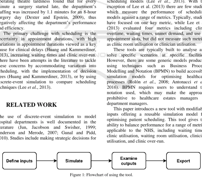
The Trust were operating two clinic models in the outpatient department; a dedicated clinic model where clinicians stay in one room for the clinical day; and a hub and spoke model where clinicians use a central hub to complete admin work (e.g. patient notes). These have a smaller number of clinic rooms to consult with patients (i.e. clinicians use any free clinic room). These clinic models can operate in parallel during a day with variable numbers of clinicians and rooms across two floors of the outpatient department. This paper details the development, inputs, simulation and outputs of the tool developed to aid clinic planning for the Trust. Figure 1 shows the process users take using the tool presented here.
3.1 Inputs
Two factors which negatively impact patient scheduling, and hospital performance, are variations in the appointment durations (i.e. the time a patient spends with a physician) and arrival times (i.e. whether a patient arrives early or late for their appointment). For appointment duration variation, an analysis of anonymised historical appointment data was performed to identify the variation. Historical data were provided for a five month period between July and November 2015 for a range of outpatient appointment types and included the arrival time of the patient, totalling 4,945 data
points. Of this, some appointments were excluded from analysis where the duration was less than five minutes or greater than 90 minutes (278), or where the appointment data were incomplete (919), for example, if it did not specify the activity undertaken. This was done to remove appointments which were logged after they occurred (i.e. typically resulting in very short appointment durations) and ones which could not be specifically linked to the outpatient services of this department. This gave a remaining total of 3,748 data points for analysis. An average (mean) appointment duration for low throughput (24mins) and high throughput (22mins) clinic models were extracted, along with the value representing one standard deviation from this mean appointment duration. Figure 2 shows the distribution of appointment durations for the low throughput model and Figure 3 shows the distribution for the high throughput model from the historical data.
The tool uses a number of inputs that define the clinic day to be analysed, ranging from the number of rooms and clinicians available, to the arrival profile of patients. The inputs are modifiable by the user at runtime, allowing them to simulate a variety of scenarios. For example, users can simulate and compare between 24 clinic rooms and 36 clinic rooms with ease. Previous academic discussion has noted that tools for this type of modelling are better understood by users if the inputs have sensible default values from the outset (Fletcher et al., 2007; Gunal and Pidd, 2010). In acknowledgement of this, the tool was developed with default values for each input derived from discussions with the Trust and analysis of the historical data. The inputs and their default values are given in Tables 1 through 4.
The inputs provide a comprehensive analysis model which evaluates the range of metrics defined by the Trust. Of these inputs, some are related to the clinician working practices and protocols. An example of this is the clinician write-up period after each appointment has been completed. This is the time in which clinicians enter details of the patient’s visit into their electronic records system, order follow-up tests, and organise referrals as necessary. For the dedicated clinic model, this occurs in the same room as the appointment undertaken by the clinician who does not leave, and so this time is taken into account in the room turnaround (the time taken for the room to be prepared for the next patient). However, for the Hub/Spoke model, this write-up time is conducted at the staff hub, allowing the room to be freed up quicker for the next patient to be seen by another clinician.
3.2 Queues
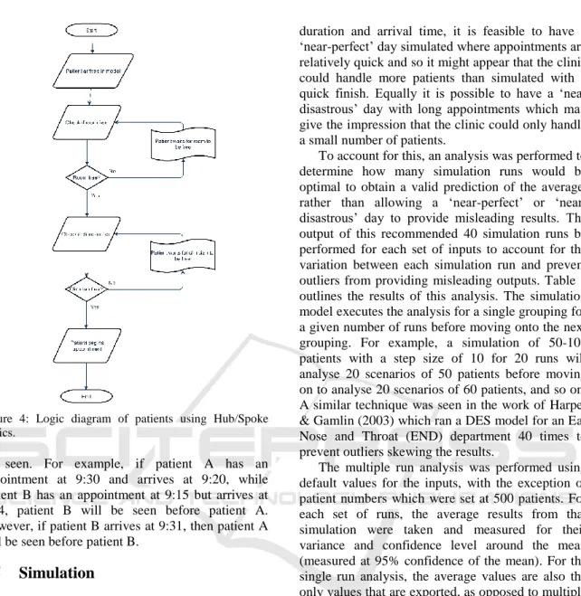
Queueing is relatively simple in the dedicated model, with patients arriving at the waiting area and then waiting for a room to be free following the room turnaround and the clinician write-up period. However, for the Hub/Spoke model queuing is slightly different, with there being a need for both a room to be empty, and a clinician to be free. The logic flow for this queue is presented in Figure 4.
Figure 2: Distribution of low throughput appointment durations.
3.3 Patient Numbers
The objective of the tool is to produce an optimal patient schedule that allows the department to examine as many patients as possible in a given day while keeping within the agreed target for a range of metrics. As such, the tool does not take in a single figure for the number of patients, but rather a range and step size. This range is analysed, increasing by the step size for each simulation run. This provides the users output for each metric for the range of patients, allowing them to compare schedules and choose the optimal with ease.
Figure 3: Distribution of high throughput appointment duration.
Table 1: Scenario inputs and default values.
Input Default value Description
Clinic hours 10 hours How many hours does the clinic wish to run for? Appointments per
day (min)
150 What is the smallest number of patients to simulate? Appointments per
day (max)
500 What is the largest number of patients to simulate? Setting the maximum to the same value as the minimum will result in a simulation run of just that number of patients, regardless of step size.
Appointment step size
50 What are the steps of patients to simulate? For the default values the patient numbers simulated are: 150, 200, 250, 300, 350, 400, 450, 500.
Booking interval 15 minutes What is the minimum amount of time between appointment slots. For example, if a clinic starts at 9am, patients are given appointments at 9am, 9:15, 9:30, 9:45, etc.
Arrival profile – percentage of early arrivals
70% How many patients will turn up early for their appointment.
Arrival profile – percentage of late arrivals
30% How many patients will turn up late for their appointment.
Arrival profile – minutes early
10 minutes How early will patients turn up for their appointment. E.G. for a 9:15 appointment a patient will arrive at 9:05.
Arrival profile – minutes late
9 minutes How late will patients turn up for their appointment. E.G. for a 9:15 appointment a patient will arrive at 9:24.
Arrival profile – for each clinic hour
Defaults as above for arrival profile
The user is given the option to define the arrival profile for each individual hour of clinic operation for greater control of the profile.
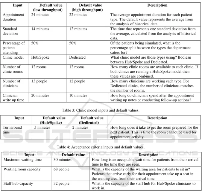
Table 2: Clinic inputs and default values. Input Default value
(low throughput) Default value (high throughput) Description Appointment duration
24 minutes 22 minutes The average appointment duration for each patient type. The default value represents the average from the analysis of historical data.
Standard deviation
14 minutes 12 minutes The time that represents one standard deviation from the average, calculated from the analysis of historical data.
Percentage of patients attending
50% 50% Of the patients being simulated, what is the percentage split between the types the department caters for?
Clinic model Hub/Spoke Dedicated What clinic model are those types using? Boolean between Hub/Spoke and Dedicated.
Number of clinic rooms
12 rooms 12 rooms How many clinic rooms are available to each clinic. If both clinics are running a Hub/Spoke model then these values are combined.
Number of clinicians
13 people 12 people How many clinicians are working each type. For Dedicated clinics, the number of clinicians matches the number of rooms.
Clinician write up time
20 minutes 10 minutes How long do clinicians spend after the appointment writing up notes or conducting follow-up actions? Table 3: Clinic model inputs and default values.
Input Default value (Hub/Spoke) Default value (Dedicated) Description Turnaround time
5 minutes 2 minutes How long does it take to get the room prepared for the next patient. This is time the room cannot be used for appointment activity.
Table 4: Acceptance criteria inputs and default values.
3.4 Arrival Profiles
Another variance which can impact on a clinic’s operational efficiency is the arrival times of patients with appointments. Patients rarely turn up for an appointment at the time of that appointment. Rather they turn up early, to ensure they make it, or are late for a variety of reasons. For this, the arrival profile can be defined by the user as a uniform profile, or define an arrival profile for each hour of the clinic’s operations. This means that if users spot a trend in patients arriving late in, for example, the afternoon, this can be built into the simulation model to analyse the impact of this.
Patients that arrive early will be registered in the model from their arrival time, and will be placed in
the queue to be seen based on their arrival. Patients that arrive ahead of their appointment timeslot earlier in the model may have the opportunity to begin their appointment prior to the scheduled appointment timeslot if a room and a clinician are free when they arrive and no other patients are in the queue ahead of them. If a room or clinician is not free however then they join the queue to be seen when the resources are available.
Patients that arrive late are processed depending on how late they arrive. For the Trust, the policy is for patients that arrive within 15 minutes of their appointment timeslot to be seen before patients with later appointments already in the queue. Effectively this allows late patients up to 15 minutes grace to jump the queue before enduring an unknown wait to
Input Default value Description
Maximum waiting time 30 minutes How long is an acceptable wait time for patients from their arrival time to the time they are seen.
Waiting room capacity 68 people What is the capacity of the waiting area for patients to sit in? Patients that arrive early for their appointment take up a seat in the waiting area from their arrival time.
Staff hub capacity 32 people What is the capacity of the staff hub for Hub/Spoke clinicians to work in.
Figure 4: Logic diagram of patients using Hub/Spoke clinics.
be seen. For example, if patient A has an appointment at 9:30 and arrives at 9:20, while patient B has an appointment at 9:15 but arrives at 9:24, patient B will be seen before patient A. However, if patient B arrives at 9:31, then patient A will be seen before patient B.
3.5 Simulation
The simulation is provided by the discrete-event simulation (DES) tool SmartProcessAnalyser, developed by BuroHappold, which builds a set of clinic rooms based on the inputs provided by the user and produces a simulation model for the first grouping of patients. This model is then executed and analysis results exported to a spreadsheet file before a new simulation model is generated for the next simulation run.
3.6 Multiple Analysis
The results of a single simulation can be misleading with the variance in appointment durations and arrival times providing a different result each simulation run. Though the tool uses a random function to generate the patient appointment
duration and arrival time, it is feasible to have a ‘near-perfect’ day simulated where appointments are relatively quick and so it might appear that the clinic could handle more patients than simulated with a quick finish. Equally it is possible to have a ‘near disastrous’ day with long appointments which may give the impression that the clinic could only handle a small number of patients.
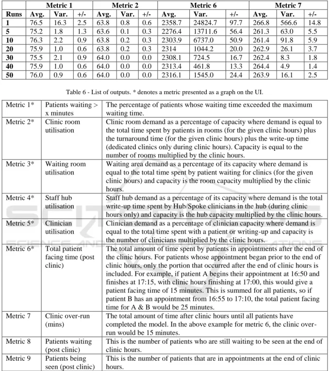
To account for this, an analysis was performed to determine how many simulation runs would be optimal to obtain a valid prediction of the average, rather than allowing a perfect’ or ‘near-disastrous’ day to provide misleading results. The output of this recommended 40 simulation runs be performed for each set of inputs to account for the variation between each simulation run and prevent outliers from providing misleading outputs. Table 5
outlines the results of this analysis. The simulation model executes the analysis for a single grouping for a given number of runs before moving onto the next grouping. For example, a simulation of 50-100 patients with a step size of 10 for 20 runs will analyse 20 scenarios of 50 patients before moving on to analyse 20 scenarios of 60 patients, and so on. A similar technique was seen in the work of Harper & Gamlin (2003) which ran a DES model for an Ear Nose and Throat (END) department 40 times to prevent outliers skewing the results.
The multiple run analysis was performed using default values for the inputs, with the exception of patient numbers which were set at 500 patients. For each set of runs, the average results from that simulation were taken and measured for their variance and confidence level around the mean (measured at 95% confidence of the mean). For the single run analysis, the average values are also the only values that are exported, as opposed to multiple runs where the average value is the average of all values in that simulation. For example, a five run simulation shows the average of each of the five results on the graph outputs. Each simulation was run 20 times, giving 20 samples for each ‘run’ being analysed, ranging from 20 simulation results (20 times 1 run) to 1000 simulation results (20 times 50 runs) in the analysis. The results shown in Table 5
show that the variance is reduced for each metric as the more simulation runs are performed, until 50 runs is reached. At this point, some metrics variance increases while others stay the same, suggesting that 40-50 runs per simulation is likely to provide a more reliable result than 1 run per simulation.
3.7 Analysis Results
The simulation exports the result of the analysis to a spreadsheet file that can be examined in full by the user and includes graphs that highlight the core results of the simulations. This includes the individual result for each simulation run for the user to inspect if they so wish. The metrics included in this tool are shown in Table 6. Each graph shows the number of simulated patients along the X-Axis, and for each patient grouping the average result after all of the simulation runs. Also given are error bars denoting the minimum result and maximum result of all runs. Figures 5 through 8 provide examples of the graph outputs following simulations using default values.
The spreadsheet of results allows users to explore the simulation results in detail. For each metric an overall value (average of both clinic models) is provided, as well as the result for each clinic model. This is given for each simulation run. For the room utilisation metrics, a detailed output of the utilisation for each clinic type (and average of overall) for each simulated minute is provided. This is broken into the three states the room may be in, idle (empty room ready for a patient), occupied (with a patient), and being turned around (prepared
for the next patient). This allows users to analyse periods of a simulated day when utilisations may be lower than anticipated.
3.8 Result Interpretation
The tool provides the graph outputs on the user interface (UI) for the user to work with as soon as all of the simulations runs are completed, with the detailed spreadsheet of data available to export. However, the tool does not interpret the results to make any recommendations of the best schedule to adopt for the clinic. Rather, this interpretation is left to the user, who can apply their experience and knowledge to weight between each metric and select the optimal patient schedule. For example, as government focus shifts towards maximising utilisation of space, it may become acceptable to have a percentage of patients waiting more than a given amount of time if the utilisation is increased. Such trade-off decisions are left to the users, with the tool providing no bias.
The error bars in the graphs shown in
Figures5 through 8 show the minimum and maximum
value of the results, with the columns denoting
the average result.
Figure 5: Percentage of patients waiting more than the acceptance criteria.
Figure 6: Clinic room utilisation.
Table 5: Analysis results for multiple runs comparison (confidence of the mean measured at 95%).
Metric 1 Metric 2 Metric 6 Metric 7
Runs Avg. Var. +/- Avg. Var. +/- Avg. Var. +/- Avg. Var. +/-
1 76.5 16.3 2.5 63.8 0.8 0.6 2358.7 24824.7 97.7 266.8 566.6 14.8 5 75.2 1.8 1.3 63.6 0.1 0.3 2276.4 13711.6 56.4 261.3 63.0 5.5 10 76.3 2.2 0.9 63.8 0.2 0.3 2303.9 6737.0 50.9 261.4 91.8 5.9 20 75.9 1.0 0.6 63.8 0.2 0.3 2314 1044.2 20.0 262.9 26.1 3.7 30 75.5 2.1 0.9 64.0 0.0 0.0 2308.1 724.5 16.7 262.4 8.3 1.8 40 75.9 1.0 0.6 64.0 0.0 0.0 2313.4 461.8 13.3 264.4 4.9 1.4 50 76.0 0.9 0.6 64.0 0.0 0.0 2316.1 1545.0 24.4 263.9 16.1 2.5
Table 6 - List of outputs. * denotes a metric presented as a graph on the UI. Metric 1* Patients waiting >
x minutes
The percentage of patients whose waiting time exceeded the maximum waiting time.
Metric 2* Clinic room utilisation
Clinic room demand as a percentage of capacity where demand is equal to the total time spent by patients in rooms (for the given clinic hours) plus the turnaround time (for the given clinic hours) plus the write-up time (dedicated clinics only during clinic hours). Capacity is equal to the number of rooms multiplied by the clinic hours.
Metric 3* Waiting room utilisation
Waiting area demand as a percentage of its capacity where demand is equal to the total time spent by patient waiting for clinics (for the given clinic hours) and capacity is the room capacity multiplied by the clinic hours.
Metric 4* Staff hub utilisation
Staff hub demand as a percentage of its capacity where demand is the total write-up time spent by Hub/Spoke clinicians in the hub (during clinic hours only) and capacity is the hub capacity multiplied by the clinic hours. Metric 5* Clinician
utilisation
Clinician demand as a percentage of clinician capacity where demand is equal to the total time spent with a patient or writing-up and capacity is the number of clinicians multiplied by the clinic hours.
Metric 6* Total patient facing time (post clinic)
The total amount of time spent by patients in appointments after the end of the clinic hours. For patients whose appointment began prior to the end of clinic hours, only the portion that occurred after the end of clinic hours is included. For example, if patient A begins their appointment at 16:50 and finishes at 17:15, with clinic hours finishing at 17:00, this would give a patient facing time of 15 minutes. This is summed for all patients, so if patient B has an appointment from 16:55 to 17:10, the total patient facing time for A & B would be 25 minutes.
Metric 7 Clinic over-run (mins)
The total amount of time after clinic hours until all patients have completed the model. In the above example for metric 6, the clinic over-run would be 15 minutes.
Metric 8 Patients waiting (post clinic)
This is the number of patients who are still waiting to be seen at the end of clinic hours.
Metric 9 Patients being seen (post clinic)
This is the number of patients that are in appointments at the end of clinic hours.
4
LIMITATIONS
Although the tool takes into account the variance in appointment durations and arrival patterns, it does not take into account other variances related to the clinicians and facility which may impact on an
appointment schedule. For example, there is only a fixed input for the length of time clinicians will spend ‘writing up’ following an appointment. However, this could be subject to variance depending on the appointment, as follow-up tests may need to be ordered, or subsequent appointments
scheduled. This variance was unable to be captured from the appointment history data used to calculate the variance in appointment durations, and so the default values for these inputs came from discussions with experienced clinicians. However, because the input is accessible to the user of the tool the write-up time can be modified if the write-up process or time changes.
Similarly, there is no variance accounted for in the room turnaround times for each clinic type. The clinic turnaround is the time it takes to prepare the room for the next patient, which may include changing bedsheets, replenishing equipment such as gloves and needles, and removing expended equipment. This variance was also unable to be captured from historical data, though it is also less likely to have as much variance as appointments and clinician work. Turning a room round for the next patient typically follows a given process for hygiene and sanitary reasons and has a fixed protocol to be followed. Thus, the impact of a variance in turnaround times is likely to be negligible. However, as with the clinician write-up input, this input is exposed to the user to be modified as they see fit.
As the tool has been built for the outpatient operations defined by the Trust, it follows a linear unchanging clinic pathway for patients from arrival to appointment to leaving the model. It does not take into account other potential activities such as blood work prior to or after the examination. However, the underlying simulation engine allows for easy adaptation at a later stage to include further activities, both clinical and non-clinical, should future scenarios warrant it. Full implementation could allow users to build their own clinic pathway for a patient, however, at present this is not a function of the tool presented here.
5
DISCUSSION
This paper has presented a clinic planning tool that is generalisable to any outpatient clinic wishing to run dedicated, Hub/Spoke, or a mixture of both clinic types, as well as incorporating variance in patient appointment durations and arrival times for a more accurate simulation. The variance for appointment durations and arrival times was calculated from 3,748 historical appointments. However, the generic inputs are open to users of the tool and thus allow for any Trust to adopt the tool to produce their own simulation results with ease. This allows the tool to be reused and prevents it being a solution for one specific problem. Rather, this tool
can be used to tackle a range of appointment scheduling problems provided sensible inputs are given, saving a Trust the time and development cost of developing their own tool.
With increasing budget restraints on the NHS, a reusable tool that can be utilised by any hospital or department is of benefit to the healthcare industry. Its generic modelling inputs, not constrained by spatial requirements, allow for reuse and easy adoption by other healthcare providers. However, its adaptability through the use of the extendable DES engine also ensures the tool can evolve with policy changes and continue to provide optimal patient schedules.
6
CONCLUSIONS
The variance in appointment durations plays a large part in the efficiency and operation of a clinic. Though there may be attempts to standardise appointment durations, variations will undoubtedly occur as individual health concerns cannot always be feasibly addressed in a strict appointment window. As such, it is better to accept the variance and plan with it, rather than to plan for no variance and wonder why clinics are over-running every day and clinicians are suffering from being overworked. This tool assists with this, taking the variance and randomness in appointment durations and building this into the simulation model from the start. The use of a generic input set-up to define the clinic model allows the tool to be applicable to any department utilising the given clinic models to find an optimal appointment schedule.
The variance in outputs generated by each individual simulation run has been highlighted as a danger of incorporating variance in appointment durations. This shows the need for multiple simulation runs to be performed on a DES model to reduce overall impact of outliers from producing non-representative results and improve the confidence in the outputs. The inclusion of clinician resources for the clinic also allows for future planning to be undertaken, by seeing the impact of clinician changes (holiday, sickness, etc.) on the system.
Finally, a range of metrics has been included in the tool, providing a comprehensive analysis to the user. The metrics offer output based on current targets and guidelines for the NHS. These can be easily adapted or added to as targets and guidelines change. The end result of using the tool is the user’s ability to produce an appointment schedule which
will allow for seeing the maximum number of patients possible in a day without negatively impacting clinic utilisation, clinician utilisation, clinic over-run, or patient waiting times.
ACKNOWLEDGEMENTS
We would like to thank the Engineering and Physical Sciences Research Council, and Centre for Innovative and Collaborative Construction Engineering at Loughborough University for provision of a grant (number EPG037272) to undertake this research project in collaboration with BuroHappold Engineering Ltd.
REFERENCES
Anderson, J. G. and Merode, G. G. (2007) ‘Special issue on health care simulation’, Health Care Management Science, 10(4), pp. 309–310. doi: 10.1007/s10729-007-9031-x.
Antonacci, G., Calabrese, A., D’Ambrogio, A., Giglio, A., Intrigila, B. and Ghiron, N. L. (2016) ‘A BPMN-based automated approach for the analysis of healthcare processes’, in Proceedings - 25th IEEE International Conference on Enabling Technologies: Infrastructure for Collaborative Enterprises, WETICE 2016, pp. 124–129. doi: 10.1109/WETICE.2016.35.
Ballard, S. M. and Kuhl, M. E. (2006) ‘The use of simulation to determine maximum capacity in the surgical suite operating room’, in Proceedings - Winter Simulation Conference, pp. 433–438. doi: 10.1109/WSC.2006.323112.
Bernstein, S., Aronsky, D., Duseja, R., Epstien, S., Handel, D., Hwang, U., McCarthy, M., McConnell, J., Pines, J., Rathlev, N., Schafermeyer, R., Zwemer, F., Schull, M. and Asplin, B. (2009) ‘The effect of emergency department crowding on clinically oriented outcomes’, Academic Emergency Medicine, 16(1), pp. 1–10. doi: 10.1111/j.1553-2712.2008.00295.x. Brenner, S., Zeng, Z., Liu, Y., Wang, J., Li, J. and
Howard, P. K. (2010) ‘Modeling and analysis of the emergency department at university of Kentucky Chandler Hospital using simulations’, Journal of
Emergency Nursing, 36(4), pp. 303–310. doi:
10.1016/j.jen.2009.07.018.
Carter, P. (2016) Operational productivity and performance in English NHS acute hospitals: Unwarranted variations. London.
Davis, K., Stremikis, K., Squires, D. and Schoen, C. (2014) ‘Mirror, mirror on the wall, 2014 update: how the US health care system compares internationally’,
New York (NY): Commonwealth Fund, 16.
Denton, B., Rahman, A., Nelson, H. and Bailey, A. (2006) ‘Simulation of a multiple operating room surgical
suite’, in Proceedings of the 38th conference on Winter simulation, pp. 414–424.
Department of Health (2013) The NHS Constitution. London.
Dexter, F. and Epstein, R. (2009) ‘Typical savings from each minute reduction in tardy first case of the day starts’, Anesthesia & Analgesia, 108(4), pp. 1262–7. doi: 10.1213/ane.0b013e31819775cd.
Fetter, R. B. and Thompson, J. D. (1965) ‘The Simulation of Hospital Systems’, Operations Research, 13(5), pp. 689–711. doi: 10.1287/opre.13.5.689.
Fletcher, A., Halsall, D., Huxham, S. and Worthington, D. (2007) ‘The DH Accident and Emergency Department model: a national generic model used locally’, Journal of the Operational Research Society, 58(12), pp. 1554–1562. doi: 10.1057/palgrave.jors.2602344. Greenroyd, F. L., Hayward, R., Price, A., Demian, P. and
Sharma, S. (2016) ‘Using Evidence-Based Design to Improve Pharmacy Department Efficiency’, HERD: Health Environments Research & Design Journal, 10(1), pp. 130–143. doi: 10.1177/1937586716628276. Gunal, M. and Pidd, M. (2006) ‘Understanding accident
and emergency department performance using simulation’, Simulation Conference, 2006. WSC 06. Proceedings of the Winter, pp. 446–452.
Gunal, M. and Pidd, M. (2010) ‘Discrete Event Simulation for Performance Modelling in Healthcare: A Review of the Literature.’, Journal of Simulation, 4(1), pp. 42– 51.
Harper, P. R. and Gamlin, H. M. (2003) ‘Reduced outpatient waiting times with improved appointment scheduling: A simulation modelling approach’, OR Spectrum, 25(2), pp. 207–222. doi: 10.1007/s00291-003-0122-x.
Harper, P. R. and Pitt, M. A. (2004) ‘On the challenges of healthcare modelling and a proposed project life cycle for successful implementation’, Journal of the Operational Research Society, 55(6), pp. 657–661. doi: 10.1057/palgrave.jors.2601719.
Health and Social Care Information Centre (2015) Estates Returns Information Collection: England 2014 to 2015. London.
Hendrich, A., Chow, M., Skierczynski, B. and Lu, Z. (2008) ‘A 36-hospital time and motion study: How do medical-surgical nurses spend their time?’, The Permanente Journal, 12(3), pp. 25–34.
Huang, Y.-L. and Kammerdiner, A. (2013) ‘Reduction of service time variation in patient visit groups using decision tree method for an effective scheduling’,
International Journal of Healthcare Technology and
Management, 14(1–2), pp. 3–21. doi:
10.1504/IJHTM.2013.055081.
Jun, J., Jacobson, S. and Swisher, J. (1999) ‘Application of discrete - event simulation in health care clinics: A survey’, Journal of the Operational Research Society,
50(2), pp. 109–123. doi:
10.1057/palgrave.jors.2600669.
Kuljis, J., Paul, R. J. and Chen, C. (2001) ‘Visualization and Simulation: Two Sides of the Same Coin?’,
Simulation, 77(3/4), pp. 141–152. doi: 10.1177/003754970107700306.
Lee, S., Min, D., Ryu, J. -h. and Yih, Y. (2013) ‘A simulation study of appointment scheduling in outpatient clinics: Open access and overbooking’,
Simulation, 89(12), pp. 1459–1473. doi:
10.1177/0037549713505332.
Leskovar, R., Accetto, R., Baggia, A., Lazarevič, Z., Vukovič, G. and Požun, P. (2011) ‘Discrete event simulation of administrative and medical processes’,
Zdravniski Vestnik, 80(5).
Marcario, A. (2006) ‘Are your hospital operating rooms “efficient”’, Anesthesiology, (2), pp. 233–243. Maviglia, S. M., Yoo, J. Y., Franz, C., Featherstone, E.,
Churchill, W., Bates, D. W., Gandhi, T. K. and Poon, E. G. (2007) ‘Cost-benefit analysis of a hospital pharmacy bar code solution.’, Archives of internal
medicine, 167, pp. 788–794. doi:
10.1001/archinte.167.8.788.
NHS England (2013) ‘The NHS belongs to the people: a call to action’, NHS England, London.
NHS England (2014) Five year forward view. London. Nicholson, D. (2009) ‘The Year: NHS chief executive’s
annual report 2008/09’, London: Department of Health, p. 47.
Quevedo, V. and Chapilliquén, J. (2014) ‘Modeling a Public Hospital Outpatient Clinic in Peru Using Discrete Simulation’.
Reynolds, M., Vasilakis, C., McLeod, M., Barber, N., Mounsey, A., Newton, S., Jacklin, A. and Franklin, B.
D. (2011) ‘Using discrete event simulation to design a more efficient hospital pharmacy for outpatients’,
Health Care Management Science, 14, pp. 223–236. doi: 10.1007/s10729-011-9151-1.
Rolón, E., García, F., Ruiz, F., Piattini, M., Calahorra, L., García, M. and Martin, R. (2008) ‘Process Modeling of the Health Sector Using BPMN: A Case Study’, in
Proceedings of the first international conference on health informatics (HEALTHINF), pp. 173–178. Vanberkel, P. T. and Blake, J. T. (2007) ‘A
comprehensive simulation for wait time reduction and capacity planning applied in general surgery’, Health Care Management Science, 10(4), pp. 373–385. doi: 10.1007/s10729-007-9035-6.
Werker, G., Sauré, A., French, J. and Shechter, S. (2009) ‘The use of discrete-event simulation modelling to improve radiation therapy planning processes’,
Radiotherapy and Oncology. Elsevier Ireland Ltd, 92(1), pp. 76–82. doi: 10.1016/j.radonc.2009.03.012. Zeng, Z., Ma, X., Hu, Y., Li, J. and Bryant, D. (2012) ‘A
Simulation Study to Improve Quality of Care in the Emergency Department of a Community Hospital’,
Journal of Emergency Nursing. Emergency Nurses Association, 38(4), pp. 322–328. doi: 10.1016/j.jen.2011.03.005.