Ideas and Tools for a Data Mining Style of Analysis

(1)

Ideas and Tools for a Data Mining Style of

Analysis

John Maindonald

July 2, 2009

Purpose and Range of Content

Data mining gathers up some of the ways in which a section of the computer scientist community has sought to respond to the impact of computer technology on the col-lection and use of data. The effects have spread across commerce, government and society, as well as across science. The same or similar technology may be used across these different areas of application.

Other responses, with much in common with data mining, have the names “machine learning”, and “analytics”. Machine learning has grown out of an engineering context, while the name “analytics” is widely used in a business context. Other such names are in use also, most of them with a focus on a specific area of application.

Data mining is sometimes presented as a collection of algorithms. Validation issues are, largely, left to one side. My intention is to widen the scope, to describe an enter-prise that builds on advances in data collection and data analysis technology in ways that pay serious regard to model validation issues. In this account, statistical consider-ations have a large role. Providing this is understood, the enterprise that is in mind can suitably be described as “data mining”.

These notes elaborate to some limited extent on points that I plan to cover in my talk, and extend into areas that will not be covered. Sections 1– 4 are important for the talk. Remaining sections are for follow-up study.

1 Resampling and Other Computer Intensive Methods

Both for the talk and for the practical sessions, there are several methodologies that will be important. These are:

Simulation: A model is proposed that generated the data. What are its statistical properties? One answer is repeated simulations. Simple uses of this idea are:

• Simulate repeated sampling of values that follow a normal distribution.

• Simulate repeated sampling of values that follow a non-normal distribution, per-haps an exponential distribution.

• Marks are placed on the circumference of a roulette wheel that divide it into three perhaps unequal parts. Labeling the outcomes A, B and C, one can simulate, eg, a result from 1000 spins.

In statistical learning contexts, theoretical accuracy assessments have limited use-fulness. It is frequently necessary to rely on empirical methods. This is especially true for classification models. Several important methods of this type will now be described.

Training/Test:

• Split data into training and test sets

• Train (NB: steps1 & 2); use test data for assessment.

This is the most widely applicable methodology. The test data can in principle be taken from the target population. If however data from the actual target is available when the model is fitted, one would want to use this for model fitting. Thus, in practice, testing on data from the actual target often has to be an “after-the-event” kind of check.

(3)

1 RESAMPLING AND OTHER COMPUTER INTENSIVE METHODS 3

TEST Training Training Training FOLD 1

TEST

Training Training Training FOLD 2

TEST

n1 n2 n3 n4

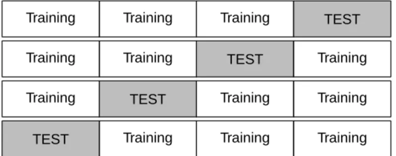
Figure 1: Schematic, designed to show how cross-validation works. For present il-lustrative purposes, data are split into four nearly equal parts, withn1,n2,n3, andn4

observations respectively. At the first iteration, then1observations in the first part are

set aside for testing, with remaining observations used for training, and so on. The split into a part that is used for testing, and the remaining observations that are used for testing, has the namefold. Once calculations for all 4 folds are complete, predicted values are available for all observations, in each case from a model that was trained independently of those observations.

When there is very adequate data, a training/test split of the data achieves all that is needed. It is not necessary to look for a method, such as will now be described, that makes better use of the data.

Cross-validation Simple version: Train on subset 1, test on subset 2 Then; Train on subset 2, test on subset 1

More generally, data are split intokparts (eg,k=10). Use each part in turn for testing, with other data used to train.

Cross-Validation Steps are:

• Split data intokparts (in Figure 1,k=4)

• At theith repeat orfold(i=1, . . .k) use:

theith part fortesting, the otherk-1 parts fortraining.

• Combine the performance estimates from thekfolds.

Bootstrap Sampling Bootstrap samples are with replacement samples, of the same size as the initial sample.

Here are two bootstrap samples from the numbers 1 . . . 10

1 3 6 6 6 6 6 8 9 10 (5 6’s; omits 2,4,5,7)

2 2 3 4 6 8 8 9 10 10 (2 2’s, 2 8’s, 2 10’s; omits 1,5,7) 1 1 1 1 3 3 4 6 7 8 (4 1’s, 2 3’s; omits 2,5,9,10)

Here is how bootstrap sampling can be used in practice:

• Take repeated (with replacement) random samples of the observations, of the same size as the initial sample.

(4)

2 KEY MOTIVATIONS 4

• Repeat analysis on each new sample (NB: In the example above, repeatboth

step 1 (selection) & 2 (analysis).

• Variability between samples indicates statistical variability.

• Combine separate analysis results into an an overall result.

2 Key Motivations

2.1 Computing Technology is Transforming Science

Computing technology is clearly transforming science. The following is a summary of the changes. All except the final item feature strongly in the data mining literature:

• Huge data sets1_{have become common. Often these hold new types of data – web}

pages, medical images, expression arrays, genomic data, NMR spectroscopy, sky maps, . . .

• Sheer size brings challenges. In the first place, these are challenges for data management. Challenges for data analysis are less simply described.

– A key question is whether there are many observations, or many variables, or both.

– Where the number of observations is large, there is often a structure (eg, changes in time) that requires attention.

• New algorithms; “algorithmic” models.

– Examples are trees, random forests, Support Vector Machines, . . .

– They are algorithmic in the sense that the motivation was algorithmic.

• Automation, especially for data collection

– There has been huge progress in automating many aspects of data analysis.

– Except however in limited areas of application, complete automation re-mains a pipe dream. In those areas where it has proved effective, automa-tion typically has a large setup and maintenance cost.

– Automation is most feasible in applications where mistakes can be toler-ated, where it is not necessary to be consistently correct.

• Synergy: computing power with new theory. Much of the new development in theoretical statistics is driven and facilitated by the demand to take advantage of new computational power.

All the above, except the final item, get strong emphasis in the data mining liter-ature. The literature emphasizes the synergy with new algorithmic development, but pretty much ignores the synergy with new developments in statistical theory.

1_{Issues of data set size have generated some modest smount cf hype, as the frequent reference to}_Big Datain Weiss and Indurkha (1997)

(5)

2 KEY MOTIVATIONS 5

2.2 Jargon – Mining, Learning and Training

Miningis used in two senses:

• Mining for data

• Mining to extract meaning is a scientific/statistical sense.

The pre-analysis data extraction & processing often relies heavily on computer technol-ogy. Additionally, there are design of data collection issues that demand more attention than has been common.

In mining to extract meaning, statistical considerations come to the fore. Computer power does however provide a major part of the “how”.

Learning & Training

• The (computing) machinelearnsfrom data.

• Usetrainingdata to train the machine or software.

Modeling (or a machine?) that learns from the data

The reference is to modeling in which the data have a substantial role in determining the form of model. The demand for such models arises, in part, from the size of the data sets (many observations) that are now commonly available. Deviations from the strict form of model that are described by theory are more readily detectable. Statisti-cal learning approaches are then used to accommodate deviations from the theoretiStatisti-cal model. The plot of residuals in Figure 2 suggests that, for the data displayed there, a statistical learning approach may be appropriate.

Time 10^−1 10^0 10^1 10^2 10^0 10^1 10^2 10^3 ●● ●●●●● ●●●● ● ● ● ● ● ●● ● ●● ●● ●● ●●● ●●● ●● ●●● ●● ● ● road ● track ● 100m 290km 9.6sec 24h Distance Resid ( lo ge scale) −0.10 −0.05 0.00 0.05 0.10 0.15 10^−1 10^0 10^1 10^2 ●●●● ●● ●● ●●●● ● ● ● ● ● ● ● ●● ●●●● ●●● ●● ● ●●●●● ●● ● ●

Figure 2: Record times versus dis-tances, both on logarithmic scales, for track and road athletic races. With a ratio of largest to smallest time that is

∼3000, differences from the line have to be large to be visually obvious. The plot of residuals shows that, for the longest race, the difference from the line is>15%. (Differences on a scale of natural logarithms, if small, are a little less than fractional differences.) There is a clear systematic pattern in the residuals.

For classification models, theory rarely gives much help in deciding on the form of model. A statistical learning approach is, to a greater or lesser extent, inherent in the nature of the modeling problem.

(6)

2 KEY MOTIVATIONS 6

In the applications of statistical learning that are prominent in the data mining lit-erature, the aim is usually prediction rather than the obtaining of interpretable model parameters. Hence the name “predictive modeling”. Interpretation of model parame-ters raises additional issues that will be the subject of brief comment in a later section.

2.3 Statistical Learning Example – Continuous Outcome

The first example (Figure 2) is for a continuous outcome variable. Data are world record times for athletic track and road races, as at October 2006. The range of dis-tances and times is huge, from 100m in 9.6sec to 292.2km in 24h.

We can fit a curve rather than a line, in what is a statistical learning approach. Here, a curve will be fitted to the residuals – this corrects for the biases in the line.

Questions are:

• Will the pattern be the same in 2030?

• Is it consistent across geographical regions?

• Does it partly reflect greater attention paid to some distances?

• So why/when the smooth, rather than the line?

Clearly the smooth curve (line, with ‘corrections’ from the line) would be useful to race organizers who wished to estimate the time at which a race winner could be expected to appear. resid(wr .lm) 10^−1 10^0 10^1 10^2 −0.10 −0.05 0.00 0.05 0.10 0.15 ●●●● ●● ● ●● ● ●●_● ● ● ● ● ● ● ●● ●●●● ●●●_●● ● ● ●●●_● ●● ● ● Distance Resid (2) −0.10 −0.05 0.00 0.05 0.10 0.15 10^−1 10^0 10^1 10^2 ● ● ● ●●● ● ●● ●●● ● ● ● ● ●●_{● ●●} ● ●●● ●●● ●● ● ● ●● ●● ●● ● ●

Figure 3: Here a smooth curve has been fitted to the residuals, using a routine that does the job pretty much automatically. It is assumed that resid-uals from the curve are independent. This assumption is especially crucial for the 95% pointwise confidence lim-its about the curve. The lower panel shows residuals from the smooth.

This is a very simple example of the use of the methodology. It generalizes, al-lowing the fitting of curves and surfaces, in principle in an arbitrary number of dimen-sions.2The ability to fit such curves and surfaces automatically is remarkable, relative to what was available a decade ago.

2.4 Statistical Learning Example – Categorical Outcome

The example relates to glass fragments that were collected in the course of forensic work. Glass was of the following types. Numbers of pieces of glass of each of the

(7)

3 PURPOSE AND SOURCE/TARGET ISSUES 7 Axis 1 Axis 2 −8 −6 −4 −2 0 2 4 −4 −2 0 2 4 6 WinF WinNF Veh Con Tabl Head

Figure 4: Visual representation of a classification rule, derived using

linear discriminant analysis, for the forensic glass data. A six-dimensional pattern of separation between the cate-gories has been collapsed down to two dimensions. Some categories may therefore be better distinguished than is evident from this figure.

different types are given:

Window float (70) Window non-float (76) Vehicle window (17) Containers (13) Tableware (9) Headlamps (29)

Variables are %’s ofNa,Mg, . . . , plus refractive index. In all there are 214 rows of data (observations)×10 columns (variables).

The aim is to find a rule that predicts the type of any new piece of glass. Figure 4 is a visual summary of the result from the use of a simple form of classification methodology, with the namelinear discriminant analysis.

Points to note are:

• The methodology is implemented within a Bayesian framework. By default, the prior probabilities for the various categories are taken to be the relative frequen-cies for those categories. The classification rule changes if the frequenfrequen-cies are changed from the default.

• For any given classification rule, the overall accuracy (proportion correctly clas-sified) changes if the prior probabilities are changed.

• For estimating the accuracy for a given target population, the prior probabilities should be the proportions in that population, not the proportions in the sample. Note that these data date from 1987. Changes since then in glass mamufacturing may well mean that they have limited relevance to current circumstances. It would be hazardous to use a prediction rule derived from these data for predictions for recently collected glass fragments.

3 Purpose and Source

/

Target Issues

A data mining style of analysis, if it is done properly, offers exactly the same range of challenges as data analysis more generally. As with any data analysis, key considera-tions are:

(8)

4 ANALYSIS TYPES AND TOOLS 8

A1: What is (are) the intended purpose(s) of the analysis?

A2: Is predictive accracy the main consideration? Or is the aim scientific of other insight, perhaps based on values of parameter estimates.

A3: How widely is it hoped that results will apply?

The answers may have strong implications for the any decision on how to handle the data. Data mining exercises typically are mainly interested in predictive accuracy. Questions of what interpretation can be placed on model parameters do however of-ten arise, ofof-ten as an afterthought to the main analysis. It is therefore important to understand the potential for misinterpretation.

Questions on which the analysis may help shed light are:

B1: Is a repeat of the analysis with a new set of data likely to turn up comparable results?

B2: How widely applicable is whatever can be learned from the data? (Will it apply to a city that is different from those that generated the sample data? Will it apply to a different time – next year, or two years’ time?)

Question B2 is the really crucial question. It asks those who analyze or use the data to think about how the target population may relate to the source population? At the extremes:

T1: Source and target may be quite different. The notion that the data can be used to make statements that apply to the target is, at the very least, hopeful!

T2: Source and target may be closely identical.

Experiments, if properly designed, should ensure that source is closely identical with a target. This is not a guarantee that source will be closely identical with the target that is of main interest. Experiments with one or other strain of mice may or may not give results that generalize to other strains. Results may or may not have relevance, or some limited relevance, to humans.

Source/target issues have particular pertinence for data mining type applications, where data are not commonly experimental.

4 Analysis Types and Tools

The favoured methodologies come, mostly, under the broad heading of “regression”. There is some use of regression methods with a continuous outcome variable. The data mining literature is however strongly focused on methodologies where the outcome is classification into one of two or more categories.

4.1 Methodologies

For work with classification data, there is some use of classical statistical tools. Such tools include logistic and multinomial logistic regression, and the closely related lin-ear and quadratic discriminant analysis approaches. Theoretical accuracy assesments, making the usual independence assumptions, are asymptotic, and may or may not be useful in practice. Commonly, accuracy is estimated using the same approaches as are used for the newer “data mining” methodologies.

(9)

4 ANALYSIS TYPES AND TOOLS 9

Prominent among the newer “data mining” methodologies that have found favour in the data mining and machine learning communities are:

• Classification trees and various extensions of trees:

– Random forests and related “bagging methods”;

– “Boosting” methods, notably Adaboost

• Support Vector Machines

• Neural networks (these turn out, however, to have close connections with logistic regression).

4.2 Accuracy assessment

Primarily, the accuracy assessment methods that are discussed here assume that the target population is essentially the same as the source population from which the data have been obtained. Even for this limited purpose, there is serious scope for getting answers that can be grossly optimistic.

Accuracy assessment is important for its own sake. It is helpful to know what the finally fitted model has been able to achieve. Unless however there is effective accuracy assessment, it will not be possible to fit a good model:

• Many methods work by starting with an initial model, which is successively refinement. Too much refinement (over-fitting) will lead to a model with reduced predictive power. It is necessary to know when to stop.

• Good accuracy assessments are required so that a model fitted using one method-ology can be compared with a model fitted using another methodmethod-ology.

4.2.1 Key Methodologies for Empirical Accuracy Assessment

In statistical learning contexts, theoretical accuracy assessments have limited useful-ness. It is frequently necessary to rely on empirical methods. This is especially true for classification models. Section 1 described the methods that will be important here.

Continuous outcome data: For regression with a continuous outcome, normal the-ory accuracy estimates can, if the independent normal error assumptions are not too badly wrong, work quite well. Note however that:

• If the model is selected from a wide class of models, or if there is extensive variable selection (e.g., select the best 3 explanatory variables out of 10), the accuracy estimates may be grossly optimistic.

• If observations are not independent, accuracy estimates may again be wrong, usually optimistic. Note however that that the situation can in special cases be rescued by choosing a more realistic model for the “error”. Some of the possi-bilities are:

– For data that are collected over time, models are available that can account for the likely sequential correlation.

(10)

5 CHALLENGES FROM SIZE OF DATASET 10

– Variation is often multi-layered – variation between different countries, variation between humans in an individual country, variation between clin-ical assessment made on the same human, and so on. Again modeling approaches are available that can account for such different sources of vari-ation.

– Spatial models are another possibility.

Empirical methods for accuracy assessment can in principal be adapted for use where there is a complex error structure. This does however require a clear understanding of the theoretical issues, and is not straightforward.

Categorical outcome data: Here, the theoretical accuracy estimates that are avail-able for certain of the methods rely on asymptotic approximations. For ‘algorithmic’ methods, including tree-based methods and random forests, theoretical results have limited relevance. Accuracy assessment almost inevitably relies on empirical methods. The empirical methods do if used correctly cope with the effects of model and variable selection.

4.2.2 Keeping Score

As has been pointed out, the source population from which data have been obtained will often not be exactly the same as the target population. There are two important issues here:

• Where predictive modeling of a comparable type is being carried out repeat-edly, the analyst should keep a record of the comparison between after-the-event model performance and predicted performance, e.g., from cross-validation on the original data.

• Often, predictions are successively made ahead in time. If a long enough data series is available, time series methods may be apprpropriate. In effect, past changes from one time to the next are used as a guide to likely future changes. The modeling of changes over time is in principle a good idea. Do not however put too much faith in the model. A lesson from the recent financial crisis is, surely, that it is unwise to put much faith in any financial model that does not allow for occasional “shocks”. The warnings in Taleb (2004) merit attention.

5 Challenges from Size of Dataset

Sheer size brings challenges. In the first place, these are challenges for data manage-ment. The analysis challenges that result from data set size are not, however, primarily those of scaling up regression and related models for use with large datasets.

The analysis challenges are most important for models with a complex error struc-ture – repeated measures and times series, spatial models, and so on. They are much less important for the use of regression models.

Some of the issues are:

• Additional structure often comes with increased size – data may be less homo-geneous, span larger regions of time or space, be from more countries

(11)

6 THE INTERPRETATION OF MODEL PARAMETERS 11

• Or there may extensive information about not much!

– e.g., temperatures, at second intervals, for a day.

– SEs from modeling that ignores this structure may be misleadingly small.

• In large homogeneous datasets, spurious effects are a risk

– Small SEs increase the risk of detecting spurious effects that arise, e.g., from sampling bias (likely in observational data) and/or from measurement error.

Where a straightforward use of a regression model really does seem appropriate, there can be advantages in structuring the analysis as a series of separate regressions:

• As an example, consider data that have been collected over a non-trivial interval of time. It is then sensible, as a check, to do separate analyses for separate times.

• Where there is no time or other such structure in the data, the analysis can use-fully be repeated for separate random samples of the data. Variation in model parameters and predictions under such repeated sampling provides a check on theoretically based estimates of standard errors. If the empirical standard errors are larger, it is those that should be believed.

6 The Interpretation of Model Parameters

Consider data3_{that gives record times for Northern Ireland mountain races.}

The “obvious” simple model has log(time) as a linear function of log(dist) and log(climb).

[

log(time)=−5.0+0.68 log(dist)+0.47 log(climb)

Note the coefficients 0.68 (for log(dist)) and 0.47 (for log(climb))! Do they make sense? Thus, the coefficient 0.68 for log(dist) implies that the relative rate of increase of time with distance is, if climb is held constant, 68% of the relative rate of increase of distance. If a second kilometer is added to a 1 kilometer race, the time per unit distance will be better than for the 1 kilometer race.

The clue is that the coefficient predicts what will happen if climb is held constant. The one kilometer race then involves much steeper climbing (and decent) than the two kilometer race.

More interpretable coefficients can be obtained by regressing on log(dist) and log(climb/dist). The comparison between different distances is then fair.

For a meaningful interpretation of model parameters, it is necessary to be sure that:

• All major variables or factors that affect the outcome have been accounted for.

• Those variables and factors operate, at least to a first order of approximation, independently.

Rosenbaum (2002) suggests approaches that are often useful in the attempt to give meaningful interpretations to coefficients that are derived from observational data.

(12)

7 NOTES ON METHODS FOR USE WITH CLASSIFICATION DATA 12 1st discriminant axis 2nd discr iminant axis −4 −2 0 2 −6 −4 −2 0 2 ● ● ● ● ● ● ● ● ● ● ● ● ● ● ● ● ● ● ● ● ● ● ● ● ● ● ● ● ● ● ● ● ● ● ● ● ● ● ● ● ● ● ● ● ● ● ● ● ● ● ● ● ● ●● ● ● ● ● ● ● ● ● ● ● ● ● ● ● ● ● ● ●● ● ● ● ● ● ● ● ● ● ● ● ● ● ● ● ● ● ● ● ● ● ●● ● ● ● ● ● ● ● ● ● ● ● ● ● ● ●● ● ● ●●_● ● ● ● ● ●● ● ● ● ●●_● ● ● ● ●_● ●● ● ● ●●● ● ● ●

overt ● chemical ● normal ●

Figure 5: This is a visual sum-mary of results from the use of linear discriminant analysis. Classification accuracy, estimated by leave-one-out cross-validation, was 89%.

7 Notes on Methods for Use with Classification Data

Many different methods are available. The data mining literature encourages wide experimentation. The stance taken here is that it is better to start with several well-understood methodologies, and get to understand those, before branching out more widely. Three methodologies will be described here – linear discriminant analysis (LDA), trees and random forests. Trees will be of interest mainly for understanding the random forest methodology.

Linear Discriminant Analysis: The implementation that will be used here islda()

in R’sMASSpackage. This methodology has the following attractions:

• It is simple, in the style of classical regression.

• It leads naturally to a 2-D plot.

• The plot may suggest trying methods that build in weaker assumptions. Details are in Section 8.

Random forests: The implementation that will be used here israndomForest()in R’srandomForestpackage. This methodology has the following attractions:

• It is clear why it works and does not overfit.

• No other method consistently outperforms it.

• It is simple, and highly automatic to use.

7.1 Example used to illustrate the methodologies

The three classes are from a clinical classification of Diabetes –overt(overt diabetic),

chemical(chemical diabetic), andnormal(normal). Can these be derived directly from five available clinical measures?

(13)

7 NOTES ON METHODS FOR USE WITH CLASSIFICATION DATA 13 | glucArea>=420.5 fpg>=117 overt chemical normal

Each tree is for a different random with replacement ('bootstrap') sample of the data, and sample of variables

Each tree has one vote; the majority wins

| fpg>=118.5 fpg>=100.5 relwt>=1.045 Insulin>=228.5 overt

chemical_chemical_normalnormal

| fpg>=117 Insulin>=294.5 overt chemical normal | fpg>=117 relwt>=1.045 fpg>=102.5 overt

chemicalchemicalnormal

| fpg>=117 SSPG>=192 overt chemical normal | glucArea>=419.5 glucArea>=656.5 overt chemical normal | fpg>=119 relwt>=1.01 overt chemical normal | glucArea>=420.5 glucArea>=596.5 overt chemical normal | glucArea>=420.5 fpg>=116 overt chemical normal | glucArea>=408 glucArea>=656.5 overt chemical normal | fpg>=117 SSPG>=150 overt chemical normal | glucArea>=422 fpg>=118.5 overt chemical normal | glucArea>=408 glucArea>=606 overt chemical normal

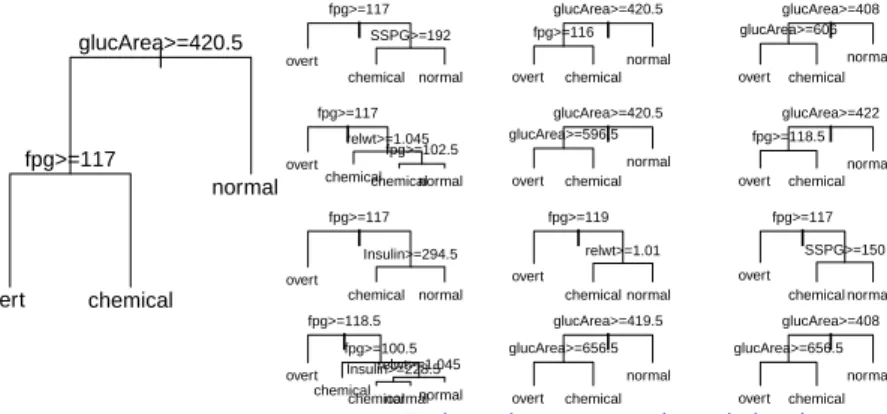
Figure 6: The left panel is a classification tree that was derived from tree-based classi-fication. Each tree in the right panel is for a different bootstrap sample of the diabetes data. Additionally, a different random sample of variables is used for each different tree. The final classification is determined by a random vote over all trees.

The clinical measures (explanatory variables) are relwt (relative weight), fpg

(fasting plasma glucose),glucArea(glucose area),Insulin(insulin area), andSSPG

(steady state plasma glucose).

Figure 5 is a visual summary of results from the use of linear discriminant analysis. The right panel shows the classification tree obtained from tree-based regression.

Tree-based classification proceeds by constructing a sequence of decision steps. At each node, the split is used that best separates the data into two groups. Here tree-based regression does unusually well (CV accuracy=97.2%), perhaps because it is well designed to reproduce a simple form of sequential decision rule that has been used by the clinicians.

How is ‘best’ defined? Splits are chosen so that the Gini index of “impurity” is minimized. Other criteria are possible, but this is howrandomForest()constructs its trees.

The random forest methodology will usually improve (but not here), sometimes quite dramatically, on tree-based classification. Figure 6 shows trees that have been fitted to different bootstrap samples of the diabetes data. Typically 500 or more trees are fitted, without a stopping rule. Individual trees are likely to overfit. As each tree is for a different random sample of the data, there is no overfitting overall.

(14)

8 LINEAR METHODS FOR CLASSIFICATION – THEORY 14 1st ordinate axis 2nd ordinate axis −0.4 −0.2 0.0 0.2 0.4 −0.4 −0.2 0.0 0.2 0.4 ● ● ● ● ● ● ●●●● ● ● ● ● ● ● ● ● ● ● ● ● ● ● ●●●●● ●●●● ● ● ● ● ● ● ● ●●● ● ● ●●●● ●● ● ● ● ● ● ● ● ●● ● ● ● ● ●● ● ● ● ● ●● ●●●●● ● ● ● ●● ● ● ●● ● ● ● ● ●●●●●●●● ● ● ● ●● ●●●●●●●●● ●●●● ●_●●●● ● ● ● ●●●● ● ● ● ● ● ● ● ●● ● ● ● ● ●● ● ●

overt ● chemical ● normal ●

Figure 7: The plot is an attempt to rep-resent, in two dimensions, the random forest result. This plot tries hard to reflect probabilities of group member-ship assigned by the analysis. It does not result from a ’scaling’ of the fea-ture space.

8 Linear Methods for Classification – Theory

See Ripley (1996); Venables and Ripley (2002); Maindonald & Braun (2007, Section 12.2).

8.1 Linear methods, vs strongly non-parametric methods

Linear methods may be contrasted with the strongly non-parametric random forest method that uses an ensemble of trees. See Maindonald & Braun (2007, Section 11.7). A good strategy for getting started on an analysis where predictive accuracy is of pri-mary importance is to fit a linear discriminant model with main effects only, comparing the accuracy from a random forest analysis. If the random forest analysis gives little or no improvement, the linear discriminant model may be hard to better. There is much more that can be said, but this may be a good starting strategy.

8.2 Notation and types of model

Observations are rows of a matrixXwithpcolumns. The vectorx, is a row ofX, but in column vector form. The outcome is categorical, one ofgclasses.

Methods discussed here will all work with monotone functions of the columns of

X. By allowing columns that are non-linear monotone functions of the initial variables, additive non-linear effects can be accommodated.

As before, observations are rows of a matrixXwithpcolumns. The vectorx, is a row ofX, but in column vector form.

The outcome is categorical, one ofg classes, where now g may be greater than 2. The matrixWestimates the within class variance-covariance matrix, whileB es-timates the between class variance-covariance matrix. Details of the estimators used are not immediately important. Note however that they may differ somewhat between computer programs.

8.3 lda()

and

qda()

The functions that will be used here arelda()andqda(), from theMASSpackage for R. The functionlda()implements linear discriminant analysis, whileqda()

(15)

imple-8 LINEAR METHODS FOR CLASSIFICATION – THEORY 15

ments quadratic discriminant analysis. Quadratic discriminant analysis is an adaptation of linear discriminant analysis to handle data where the variance-covariance matrices of the different classes are markedly different. Forg=2 the logistic regression model, fitted using R’sglm()function, is closely analagous to the linear discriminant model, fitted usinglda().

An attractive feature oflda() is that it yields “scores” that can be plotted. Let

r = min(g−1,p). Recall that pis the number of columns of a version of the model matrix that lacks an initial column of ones. Then assuming thatXhas no redundant columns, there will bersets of scores. Thersets of scores can be examined using a pairs plot. Often, most of the information is in the fist two or three dimensions. Such plots may be insightful even for data wherelda()is inadequate as a classification tool.

8.3.1 lda()andqda()– theory

The functionslda()andqda()in theMASSpackage implement a Bayesian decision theory approach.

• A prior probabilityπcis assigned to thecth class (i=1, . . .g).

• The densityp(x|c) ofx, conditional on the classc, is assumed multivariate nor-mal, i.e., rows ofXare sampled independently from a multivariate normal dis-tribution.

• For linear discrimination, classes are assumed to have a common covariance matrixΣ, or more generally a common p(x|c). For quadratic discrimination, differentp(x|c) are allowed for different classes.

• Use Bayes’ formula to derive p(c|x). The allocation rule that gives the largest expected accuracy chooses the class with maximalp(c|x); this is the Bayes’ rule.

• More generally, assign cost Li j to allocating a case of class i to class j, and

choosecto minimizeP

iLicp(i|x).

Note thatlda()andqda()use the prior weights, if specified, as weights in com-bining the within class variance-covariance matrices.

Using Bayes’ formula

p(c|x) = πcp(x|c)

p(x)

∝ πcp(x|c)

The Bayes’ rule maximizesp(c|x). For this it is sufficient, for any givenx, to maximize

πcp(x|c)

or, equivalently, to maximize

log(πc)+log(p(x|c))

Now assumep(x|c) is multivariate normal, i.e.,

p(x|c)=(2π)p2 _|Σ_c_|₎−12_exp₍₋1

(16)

8 LINEAR METHODS FOR CLASSIFICATION – THEORY 16

where

Qc=(x−µc)TΣ−c1(x−µc)

Then

log(πc)+log(p(x|c))=log(πc)−

1 2Qc+ p 2log(2π)− 1 2log(|Σc|)

Leaving offthe log(2π) and multiplying by -2, this is equivalent to minimization of

Qc+log(|Σc|)−2 log(πc)=(x−µc)TΣ−c1(x−µc)+log(|Σc|)−2 log(πc)

The observationxis assigned to the group for which

(x−µ_c)TΣ−c1(x−µc)+log(|Σc|)−2 log(πc)

is smallest.

Setµc=x¯c, and replace|Σc|by an estimateWc.

[Note that the usual estimate of the variance-covariance matrix (or matrices) is positive definite, providing that the same observations are used in calculating all elements in the variance-covariance matrix andXhas no redundant columns.]

Thenxis assigned to the group to which, after adjustments for possible differences inπcand|Σc|, the Mahalanobis distance

(x−x¯c)TWc−1(x−x¯c)

ofxfromxcis smallest.

If a common variance-covariance matrixWc=Wcan be assumed, a linear

trans-formation is available to a space in which the Mahalanobis distance becomes a Eucliean distance. Replacexby

z=(UT)−1x

and ¯xcby ¯zc =(UT)−1x¯cwhereU is an upper triangular matrix such thatUTU = Σ.

Then

(x−µ_c)TW−1(x−µ_c)=(z−¯zc)T(z−z¯c)

which in the new space is the squared Euclidean distance to fromzto ¯zc.

Note: For estimation of the posterior probabilities, the simplest approach is that de-scribed above. Thus, replace p(c|x;θ) by p(c|x; ˆθ) for calculation of posterior prob-abilities (the ‘plug-in’ rule). Here, θ is the vector of parameters that must be es-timated. The R functions predict.lda() andpredict.qda() offer the alterna-tive estimatemethod="predictive", which takes account of uncertainty inp(c|x; ˆθ). Note also method="debiased", which may be a reasonable compromise between

method="plugin"andmethod="predictive"

8.4 Canonical discriminant analysis

Here we assume a common variance-covariance matrix. As described above, replacex

by

z=UT−1x

(17)

The between classes variance-covariance matrix becomes ˜

B=UT−1BU−1

The ratio of between to within class variance of the linear combinationαT_z_{is then}

αT_B_˜_α

˜

αTα_˜

The matrix ˜Badmits the principal components decomposition ˜

B=λ1u1uT1 +λ2u2uT2 +. . .+λruruTr

The choiceα=u1maximizes the ratio of the between to the within group variance, a

fractionλ1of the total. The choiceα=u2accounts for the next largest proportionλ2,

and so on.

The vectorsu1, . . .urare known as “linear discriminants” or “canonical variates”.

Scores, which are conveniently centered about the mean over the data as a whole, are available on each observation for each discriminant. These locate the observations inr-dimensional space, whereris at most min(g−1,p). A simple rule is to assign observations to the group to which they are nearest, i..e., the distancedcis smallest in

a Euclidean distance sense.

For plotting in two dimensions, one takes the first two sets of discriminant scores. A pointzithat is represented as

ζi1u1+ζi2u2+...+ζirur

is plotted in two dimensions as (ζi1, ζi2), or in three dimensions as (ζi1, ζi2, ζi3). The

amounts by which the original columns ofxineed to be multiplied to giveζi1are given

by the first column of the list elementscalingin theldaobject. Forζi2, the elements

are those in the second column, and so on. See the example below.

As variables have been scaled so that within group variance-covariance matrix is the identity, the variance in the transformed space is the same in every direction. An equal scaled plot should therefore be used to plot the scores.

8.4.1 Linear Discriminant Analysis – Fisherian and other

Fisher’s linear disciminant analysis was a version of canonical discriminant analysis that used a single discriminant axis. The more general case, where there can be as many asr=min(g−1,p) discriminant functions, is described here.

The theory underlyinglda()assignsxto the class that maximizes the likelihood. This is equivalent to choosing the class cthat minimizesdc+log(πc), where if the

same estimates are used forWandB,dcis the distance as defined for Fisherian linear

discriminant analysis. Recall thatπcis the prior probability of classc.

The output fromlda()includes the list elementscaling, which is a matrix with one row for each column ofXand one column for each discriminant function that is calculated. This gives the discriminant(s) as functions of the values in the matrixX.

8.4.2 Example – analysis of the forensic glass data

The data framefglin theMASSgives 10 measured physical characteristics for each of 214 glass fragments that are classified into 6 different types.

(18)

library(MASS}

fgl.lda <- lda(type ˜ ., data=fgl)

scores <- predict(fgl.lda, dimen=5)$x # Default is dimen=2 ## Now calculate scores from other output information

checkscores <- model.matrix(fgl.lda)[, -1] %*% fgl.lda$scaling ## Center columns about mean

checkscores <- scale(checkscores, center=TRUE, scale=FALSE) plot(scores[,1], checkscores[,1]) # Repeat for remaining columns ## Check other output information

fgl.lda

93% of the information, as measured by the trace, is in the first two discriminants.

8.5 Two groups – comparison with logistic regression

Logistic regression, which can be handled using R’s functionglm(), is a special case of a Generalized Linear Model (GLM). The approach is to model p(c|x; ˆθ) using a parametric model that may be the same logistic model as for linear and quadratic dis-criminant analysis.

In this context it is convenient to change notation slightly, and giveXan initial column of ones. In the linear model and generalized linear model contexts,Xhas the name “model matrix”.

The vectorxis a row ofX, but in column vector form. Then ifπis the probability of membershipin the second group, the model assumes that

log(π/(1−π)=β0x

whereβis a constant.

Compare logistic regression with linear discriminant analysis:

• Inference is conditional on the observedx. A model for p(x|c) is not required. Results are therefore more robust against the distributionp(x|c).

• Parametric models with “links” other than the logit f(π) = log(π/(1−π) are available. Where there are sufficient data to check whether one of these other links may be more appropriate, this should be done. Or there may be previous experience with comparable data that suggests use of a link other than the logit.

• Observations can be given prior weights.

• There is no provision to adjust predictions to take account of prior probabilities, though this can be done as an add-on to the analysis.

• The fitting procedure minimizes the deviance, which is twice the difference be-tween the loglikelihood for the model that is fitted and the loglikelihood for a ‘saturated’ model in which predicted values from the model equal observed val-ues. This does not necessarily maximize predictive accuracy.

• Standard errors and Wald statistics (roughly comparable tot-statistics) are pro-vided for parameter estimates. These are based on approximations that may fail if predicted proportions are close to 0 or 1 and/or the sample size is small.

(19)

REFERENCES 19

8.6 Linear models vs highly non-parametric approaches

The linearity assumptions are restrictive, even allowing for the use of regression spline terms to model non-linear effects. It is not obvious how to choose the appropriate de-gree for each of a number of terms. The attempt to investigate and allow for interaction effects adds further complications. In order to make progress with the analysis, it may be expedient to rule out any but the most obvious interaction effects. These issues affect regression methods (including GLMs) as well as discriminant methods.

On a scale in which highly parametric methods lie at one end and highly non-parametric methods at the other, linear discriminant methods lie at the non-parametric end, and tree-based methods and random forests at the non-parametric extreme. An attrac-tion of tree-based methods and random forests is that model choice can be pretty much automated.

8.7 Low-dimensional Graphical Representation

In linear discriminant analysis, discriminant scores in as many dimensions as seem necessary are used to classify the points. These scores can be plotted. Each pair of dimensions gives a two-dimensional projection of the data. If there are three groups and at least two explanatory variables, the two-dimensional plot is a complete summary of the analysis. Even where higher numbers of dimensions are required, two dimensions may capture most of the information. This can be checked.

With most other methods, a low-dimensional representation does not arise so di-rectly from the analysis. The following approach, which can be used didi-rectly with random forests, can be adapted for use with other methods. The proportion of trees in which any pair of points appear together at the same node may be used as a measure of the “proximity” between that pair of points. Then, subtracting proximity from one to obtain a measure of distance, an ordination method can be used to find a representation of those points in a low-dimensional space.

References

Berk, R. 2008.Statistical Learning from a Regression Perspective.

[Berk’s insightful commentary injects needed reality checks into the discussion of data mining and statistical learning.]

Maindonald, J.H. 2006. Data Mining Methodological Weaknesses and Suggested Fixes. Proceedings of Australasian Data Mining Conference (Aus06)’4

Maindonald, J. H. and Braun, W. J. 2007.Data Analysis and Graphics Using R – An Example-Based Approach.2nd_{edn, Cambridge University Press.}5

[Statistics, with hints of data mining!]

Ripley, B. D. 1996. Pattern Recognition and Neural Networks. Cambridge University Press.

Venables, W. N. and Ripley, B. D. 2002. Modern Applied Statistics withS. Springer-Verlag, 4edn.

4_{http://www.maths.anu.edu.au/˜johnm/dm/ausdm06/ausdm06-jm.pdf}_and

http://wwwmaths.anu.edu.au/˜johnm/dm/ausdm06/ohp-ausdm06.pdf

5

(20)

REFERENCES 20

Rosenbaum, P. R., 2002. Observational Studies. Springer, 2ed. [Observational data from an experimental perspective.]

Taleb, Naseem, 2004. Fooled By Randomness: The Hidden Role Of Chance In Life And In The Markets.Random House, 2ed.

[Has many insightful comments about the over-interpretation of phenomena in which randomness is likely to have a large role.]

Wood, S. N., 2006. Generalized Additive Models. An Introduction with R. Chapman & Hall/CRC.

[This has an elegant treatment of linear models and generalized linear models, as a lead-in to methods for fitting curves and surfaces.]

Ideas and Tools for a Data Mining Style of Analysis