A COMPARATIVE STUDY OF NEURAL MODELS
FOR POLYPHONIC MUSIC SEQUENCE TRANSDUCTION
Adrien Ycart
∗Daniel Stoller
∗Emmanouil Benetos
Centre for Digital Music, Queen Mary University of London, UK
{a.ycart,d.stoller,emmanouil.benetos}@qmul.ac.uk
ABSTRACT
Automatic transcription of polyphonic music remains a challenging task in the field of Music Information Retrieval. One under-investigated point is the post-processing of time-pitch posteriograms into binary piano rolls. In this study, we investigate this task using a variety of neural network models and training procedures. We introduce an adversar-ial framework, that we compare against more traditional training losses. We also propose the use of binary neuron outputs and compare them to the usual real-valued outputs in both training frameworks. This allows us to train net-works directly using the F-measure as training objective. We evaluate these methods using two kinds of transduc-tion networks and two different multi-pitch detectransduc-tion sys-tems, and compare the results against baseline note-tracking methods on a dataset of classical piano music. Analysis of results indicates that (1) convolutional models improve re-sults over baseline models, but no improvement is reported for recurrent models; (2) supervised losses are superior to adversarial ones; (3) binary neurons do not improve results; (4) cross-entropy loss results in better or equal performance compared to the F-measure loss.
1. INTRODUCTION
Automatic music transcription (AMT) is a core MIR prob-lem [25]. Its aim is to extract what is played in a music signal into a human-readable score. Much of the literature has focused on the intermediate goal of detecting when and which notes were played, also called multi-pitch detection and note-tracking. It is a long-discussed topic, yet, unless it is constrained to a specific instrument and instrument model [17], it remains a challenging task, in particular in the case of polyphonic music [2].
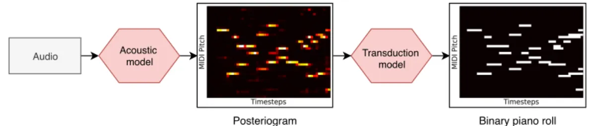
Many AMT systems use a two-step workflow [3, 13]. First an acoustic modelestimates the pitches present in each audio frame and produces a non-binary posteriogram representation over time and pitch. Then a post-processing step is applied to obtain a binary piano-roll representation,
∗Authors 1 and 2 contributed equally to this work.
c
Adrien Ycart, Daniel Stoller, Emmanouil Benetos. Li-censed under a Creative Commons Attribution 4.0 International License (CC BY 4.0). Attribution: Adrien Ycart, Daniel Stoller, Emmanouil Benetos. “A Comparative Study of Neural Models for Polyphonic Music Sequence Transduction”, 20th International Society for Music Information Retrieval Conference, Delft, The Netherlands, 2019.
or a MIDI-like note-based representation (we focus here on piano-roll representation). The former task has been extensively discussed in the literature, but the latter has received much less attention.
Recent transcription and transduction models are com-monly neural networks trained with a traditional maximum likelihood framework that assumes pitches to be indepen-dent [20, 23, 41]. Although this provides a simple and sta-ble training loss, it can lead to unrealistic estimates as the model tries to cover all the modes of the output probability distribution [35]. More recently, Generative Adversarial Networks (GANs) [18] were proposed to rectify this issue, as they do not rely on an explicit likelihood and tend to-wards realistic outputs with high likelihood under the true output distribution. In GANs, ageneratornetwork makes its outputs as realistic as possible while a discriminator
classifies examples as real (from the training set) or fake (created by the generator), which in turn gives feedback to improve the generator. GANs have made a breakthrough in high-quality image generation and reconstruction [8], and were subsequently also applied to symbolic music gener-ation [39] and singing voice separgener-ation [36]. For AMT, GANs could help produce better transcriptions by taking into account correlations across both time and pitch.
The output of neural networks used in previous ap-proaches [20,23,41] is real-valued to enable training by gra-dient descent.To obtain a piano roll at test time, the network outputs are binarised with a threshold as a post-processing step. However, this can lead to overly-fragmented notes, as in [41], when the output values are close to the thresh-old. Binary neurons [4] offer an alternative by integrating the binarisation of outputs into training while still allowing gradient back-propagation.
In this paper, we perform a comparative study of various neural-network-based methods for polyphonic sequence transduction, focusing on classical piano music. We sys-tematically compare the influence of certain design choices, namely the network architecture, the training loss and the type of outputs. In particular, we introduce a GAN frame-work and assess its performance by comparing it to simpler training losses such as cross-entropy. We also evaluate whether binary neurons can bring improvements in this con-text as suggested for symbolic music generation [15] by making generator outputs binary and thus more similar to the real examples. In addition, we propose a method to directly use the F-measure as a training objective by us-ing binary neurons. Each of these methods is evaluated with both a recurrent neural network (RNN) and a novel
convolutional network as transduction model. These de-sign choices are evaluated using inputs from two different multi-pitch detection systems (a piano-specific [23] and a multi-instrument acoustic model [5]). All experiments are conducted using a representation based on 16th note time steps, which can improve results [41] and reduce the input dimensionality compared to regular timesteps in the order of 10ms and thus the required training and test time.
Our paper is organised as follows. In Section 2, we describe previous work. Section 3 presents the dataset used. In Section 4, we detail the architecture used for our various sub-models, and the training objectives are described in Section 5. We present our evaluation metrics in Section 6, and describe our experiments and their results in Section 7. Finally, we discuss the limitations of our proposed methods along with future directions in Section 8.
2. RELATED WORK 2.1 Polyphonic Music Sequence Transduction
AMT acoustic models yield a posteriogram, which is a real-valued time-pitch representation that reflects the likelihood of pitches being present at different points in time, either as probabilities (between 0 and 1) or as saliences (unbounded). Polyphonic music sequence transduction aims to convert these posteriograms into a binary piano-roll representation (also callednote tracking). Aside from simply threshold-ing the posteriogram, one of the most popular methods involves pitch-wise Viterbi decoding [31], where each pitch is considered as a 2-state (on/off) hidden Markov model (HMM).
More recently, a series of neural network-based meth-ods has been proposed. In [6], a model combining a Re-stricted Boltzmann Machine (RBM) with a recurrent neural network (RNN) was proposed for symbolic music mod-elling. It was later used for AMT [7], using an audio rep-resentation from a Deep Belief Network as input. The same architecture was also used as a language model for piano-roll post-processing [34], to evaluate the likelihood of symbolic sequences rather than using it as a transduc-tion model. In [41], a simpler Long Short-Term Memory (LSTM) model achieved improved performance when using musically-relevant time steps, but mostly because resulting outputs are quantized to the ground truth metrical grid.
2.2 Generative Adversarial Networks
Since their introduction in 2014, GANs have enjoyed con-siderable attention [18]. The main appeal in using GANs is that the model’s likelihood only needs to be implicitly defined [29]. In contrast, defining a suitable and tractable likelihood function is difficult for complex output spaces such as the space of natural images, so simplistic assump-tions are often made about the output density. In our con-text, a GAN could generate a coherent segment of music in one pass through the network, while other methods either have to assume independent outputs for each pitch and time-frame [17,20,23,41], or condition each output dimension on all previous ones in an auto-regressive fashion [34], which requires a computationally intensive decoding process.
Applications of GANs are increasing rapidly and cover a wide variety of fields [32, 36]. For music modelling, this includes the C-RNN-GAN [28], which uses an RNN to output note events with continuous duration, onset time, pitch and velocity, instead of the discrete values used in the MIDI representation. The MuseGAN [14] generates dis-crete piano-roll music representations. Here, a continuous-output generator is used and the training data is simply treated as being continuous despite its discrete nature.
GANs can also be used for conditional prediction mod-els [26, 35, 36], where the output space is complex and high-dimensional and defining a suitable loss function is difficult. For these reasons we investigate GANs for AMT in this paper.
2.3 Binary neurons
Training a network with discrete outputs is challenging be-cause back-propagation does not yield gradients from non-differentiable operations. Various methods have been pro-posed to solve that issue, such as REINFORCE [27,37], and the straight-through estimator [4, 21]. Binary neurons were used with GANs in the context of music generation [15], as it is very easy for the discriminator to separate binary, real samples from generated ones that have real values between 0and1. This can make generator training ineffective, as the discriminator’s feedback focuses on only making the real-valued generator outputs more binary. They are re-ported as improving over a similar system with non-binary outputs [15] by being easier to train and yielding better results. More generally, binary outputs are appealing in our context, as they integrate the thresholding process into the network, removing the need for thresholding real-valued network outputs to obtain a binary piano-roll representation at test time and finding an optimal threshold value on an extra validation set.
3. DATASET
For our experiments, we use the MAPS dataset [16]. It contains MIDI files of polyphonic piano music, along with aligned audio renditions, generated using synthetic pianos and a Disklavier acoustic piano. It contains 238 pieces of classical music (18h total duration), with some pieces per-formed more than once, on different pianos. We split it into training, validation and test sets similarly to [23], where the test set features only acoustic piano and the training set only synthetic piano recordings, to obtain realistic performance estimates. We also ensure there is no overlap of pieces between the training and test set, and create a validation set by removing 10 random examples from the training set.
Rhythm annotations for this dataset are available in the A-MAPS annotations [40]. We use these annotations, in order to run our experiments using a time step of a 16th note. There are two main reasons for that choice. First, it was shown in [41] that using a 16th note time step can improve transcription performance over time steps of a fixed frame duration in seconds. Moreover, using 16th note time steps instead of fixed steps (usually on the order of 10 ms) results in a much more compact representation and faster training,
Audio Acoustic
model Transduction model
Posteriogram Binary piano roll
Figure 1. Overview of the whole transcription process. We focus on the second step. enabling large-scale experiments. However, it introduces
some imprecision when dealing with extra-metrical notes and tuples. In addition, the required beat positions are not usually available as annotations and would thus have to be obtained with a beat-tracking algorithm. Since we use beat annotations in our study, lower results than the ones reported here might be obtained in the presence of beat-tracking errors.
4. MODELS
The general workflow for our task is described in Figure 1. First an acoustic model produces a non-binary posteriogram. Then, this posteriogram is converted into a binary piano roll by a transduction model. Although this study focuses on the latter, we present both in this section.
4.1 Acoustic models
We use our transduction models with two different kinds of acoustic model outputs. The first model, described in [23], is a convolutional neural network (CNN) operating on spectrograms with logarithmically-spaced frequency bins and log-magnitude. It was designed specifically for piano transcription, and was trained on the MAPS dataset. At each time step, it outputs predictions forNp= 88pitches
as probabilities between 0 and 1. We call this modelKelz. The second model, described in [5], also uses CNNs, with a custom input representation that stacks harmonically-shifted Constant-Q transform representations of the signal. It was designed as a general multi-pitch detection system, and was trained on a multi-instrument dataset that includes piano. Besides, it has a frequency resolution of 20 cents, and has a smaller frequency span than a piano keyboard. In order to adapt it for piano transcription, we average the frequency bins that correspond to a given MIDI pitch. In this case,Np = 73. It has to be noted that this averaging
leads to lower activations. We call this modelBittner. In both cases, outputs are then downsampled to a 16th note time step. To do so, we use the best-performing method in [41] referred to asstep: letMandN be the original and downsampled posteriograms respectively, pa pitch, na 16th note step, andiandjthe time steps corresponding to
nandn+ 1respectively, we have:
s=i+round(j−i
4 ), N[p, n] =
Ps
k=iM[p, k]
s−i+ 1
4.2 Transduction model architectures
Our transduction models take the output of an acoustic model as input and are trained independently from the acoustic models. We compare two different kinds of transduction models. The first model is a Long Short-Term Memory (LSTM) network [22] with the same architecture as described in [41]. It hasNp inputs per time step, one
hidden layer with 100 hidden nodes, followed by a fully connected layer withNpoutputs.
The second model is a newly-designed CNN that uses a series of convolutions with filter sizes (1)5×5, (2)5×1 with dilation of12×1, and (3)5×15, to capture both frequency and temporal correlations. A1×1convolution processes the combined output from convolutions (2) and (3), whose output is combined with the output from convo-lution (1) using another1×1convolution. While all above convolutions have32channels and use LeakyReLU activa-tions, the final1×1convolution has only one filter and does not use an activation. Both models are closely matched in terms of the number of parameters at about80,000.
4.3 Real-valued vs. Binary outputs
We use two different strategies to convert the unnormalised, real-valued outputs obtained from the model. The first one is real-valued sigmoid outputs: the output of the network for each pitch is simply sent through a sigmoid. At test time, the outputs are binarised using a single threshold for all pitches, chosen to maximise frame-wiseFon the valida-tion set. The second strategy employs deterministic binary neurons, as described in [14]. Here, the output of the net-work for each pitch is sent through a sigmoid, and then thresholded at 0.5. This thresholding operation, however, is not differentiable, which makes it impossible to use gradient descent as training method. Therefore, we use the sigmoid-adjusted straight-through estimator [12], that was shown to provide good results [14]. It ignores the thresholding op-eration during back-propagation and instead multiplies the current gradient by the derivative of the sigmoid function.
4.4 Baseline methods
We compare our system against two baseline post-processing methods. The first binarises all outputs using a threshold optimised as explained in Section 4.3 (as op-posed to using a fixed threshold of0.5as done in [23]). The second one, introduced in [31], and later used in various systems [10, 11], is to model each pitch by an on/off HMM, and then decode the most likely sequence of hidden states using the Viterbi algorithm. The initial probabilities and
transition parameters are computed from ground truth anno-tations, one set of parameters per pitch. The observations for ‘on’ and ‘off’ states are modelled as beta distributions, each fitted to the acoustic model outputs on the validation dataset. These distributions are fitted using data from all pitches and shared between them due to the rarity of ex-tremely low and high pitches.
5. TRAINING OBJECTIVES
The networks are trained using the Adam optimiser [24] on sequences of 64 timesteps. For cross entropy and F-measure, we use a learning rate of10−2, as advised in [41].
With GANs, the learning rate is10−3for the discriminator,
and5·10−4for the generator. Early stopping is used: after
no improvement in validation framewiseFfor 30,000 iter-ations (checked every 1000 iteriter-ations), training is stopped and the best model is kept.
5.1 Cross-entropy loss
As a commonly used baseline objective, we use the binary cross-entropy (CE) loss averaged over all entriesyˆtin the
predicted piano-rollyˆas loss for the transducer model:
E(x,y)∼Pd 1 NtNp Np X p=1 Nt X t=1 yt,plog ˆyt,p+ (1−yt,p) log(1−yˆt,p) (1) whereyt,p ∈ {0,1}indicates whether a note at timestep t ∈ J1, NtKwith pitch indexp ∈ J1, NpK is active, and Pddenotes the joint distribution of acoustic model outputs
and transcriptions. While this loss is conceptually simple and allows fast and stable training, it relies on the strong assumption that each note activity can be determined inde-pendently from all others, although some note combinations are more likely to occur than others. Since the model can-not assign high probability to specific can-note combinations, only to individual notes, it would assign high probability to all involved notes. Unrealistic note combinations might then be obtained when independently sampling from these probabilities.
5.2 F-measure loss
In most cases, transduction and transcription models are trained with CE, but finally evaluated with frame- or note-wise F-measure. To close this gap between training and test-ing, we propose maximising the F-measure directly during training. However, this requires a binary piano roll instead of real-valued network outputs. As a solution, we employ binary neurons introduced in Section 4.3. By replacingP andRin the formula forFby their complete expressions (see Section 6), simplifying the equation, and using the two identitiesTP(t) =PNp
p=1yt,p·yˆt,pandFN(t) + FP(t) = PNp
p=1|yt,p−yˆt,p|whereTP(t),FP(t)andFN(t)are the
numbers of true positives, false positives and false negatives at time stept, respectively, we obtain
F= PNt t=1 PNp p=12·yt,p·yˆt,p PNt t=1 PNp p=1 2·yt,p·yˆt,p+|yt,p−yˆt,p| (2)
as our F-measure loss, which only makes use of differen-tiable operators. The only exception is the absolute value function, whose gradient is undefined only at0, which oc-curs in the above equation ifyt,p = ˆyt,p. Since the model
outputyˆt,pdoes not need to change in that case, we assign
it a gradient of0. In conjunction with binary outputs, we can thus use gradient descent to maximiseF. It has to be noted that a similar, non-binary version of F-measure was proposed as training loss in [30]. We only investigate the binary F-measure here.
5.3 Adversarial loss
We adapt the improved Wasserstein GAN [19] framework for the adversarial loss to our conditional generation case, by using a discriminator networkDθ:x, y→Rthat takes
a transcriptionyas input with the corresponding acoustic model outputxas condition. It is trained to output scalar values that minimise the loss (see Equation (3) in [19]):
L(θ) =Ex∼Pr[Dθ(x, Gφ(x))]−Ex,y∼Pd[Dθ(x, y)]
+λEx∼Pr,ˆy∼Pi(x)[(||∇yˆDθ(x,yˆ)||2−1)
2], (3)
wherePrdenotes the distribution of real acoustic model
out-puts. The third term regularises the discriminator network responses to stabilise generator training. It is weighted by the scalar hyper-parameterλ(we useλ= 10), and involves drawingPi(x), which yieldsyˆ=r·Gφ(x)+(1−r)·ywith
a weightruniformly chosen from[0,1]that interpolates between the generator outputGφ(x)and the ground truth
transcriptionyfor the inputx.
During training, the generator is updated once using the negative of the first term in (3) as loss, before the discrim-inator is trained on (3) for 5 iterations to re-estimate the Wasserstein distance between real and generator samples.
As discriminator, we use a convolutional network similar to [42]. First, a5×1convolution with dilation of12and 16channels is computed to capture relationships between octaves, and concatenated to the input features for further processing. Afterwards, a3×3convolution with a stride of two is applied four times, using 16, 32, 64, and 128 filters, respectively. The downsampled feature map is processed by a dense layer with16nodes, and by another dense layer with a single output and linear activation. All layers except the final one use LeakyReLU activations.
6. EVALUATION METRICS
We evaluate the performance of our system using the com-mon MIREX transcription metrics [1], in both frame-wise and note-wise configurations. Withframe metrics, the out-put and the ground truth are compared frame-by-frame. The metrics are computed directly on the 16th-note-timestep piano-rolls. Withnote metrics, the system output and the ground truth are viewed as a list of notes. A note is correctly detected if its pitch matches the ground truth and its onset is within a tolerance threshold of the correct onset. The threshold usually used is 50ms, however, since we operate on 16th note timesteps, we require that onset times corre-spond exactly to the ground truth. The offsets are usually
Cross-entropy F-Measure WGAN WGAN-Binary −0.050 −0.025 0.000 0.025 0.050 F ramewise F imp rovement * Kelz
Cross-entropy F-Measure WGAN WGAN-Binary
−0.3 −0.2 −0.1 0.0 0.1 Bittner Transduction model LSTM CNN HMM
Cross-entropy F-Measure WGAN WGAN-Binary
−0.05 0.00 0.05 Notewise F imp rovement Kelz
Cross-entropy F-Measure WGAN WGAN-Binary
−0.1 0.0 0.1 Bittner Transduction model LSTM CNN HMM
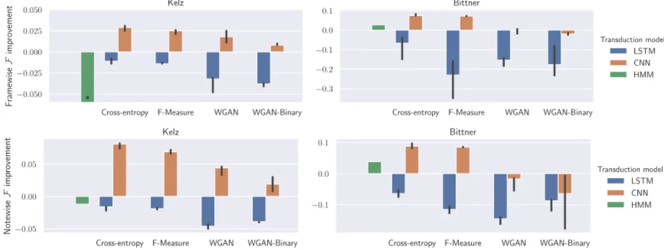
Figure 2. Model comparison across training objectives, transducer and acoustic models. Bars correspond to median improvement over simple thresholding, error bars correspond to maximum and minimum improvement across runs. * means that the bar was truncated for readability purposes.
not taken into account as they are difficult to estimate prop-erly with percussive sounds such as piano notes. We use themir_evalimplementation [33] to find the maximal match between the two lists. In both cases, the precision (P), recall (R) and F-measure (F) are computed as per [1]. These metrics are computed for each recording, and then averaged over sets of recordings.
7. RESULTS
We evaluate every possible combination of acoustic and transduction model as well as training loss and output type (continuous or binary neurons). To account for variability in training, we run every experiment 3 times and report results of the model that reaches the median frameFperformance. To assess differences in performance across different condi-tions, we perform paired Wilcoxon signed-rank tests using the piece-wise results from each median model. All median results are given in Table 1 for Kelz, and Table 2 for Bittner. We also plot the absolute improvement over simple thresh-olding for frame and noteFin Fig. 2. The error bars show the best and worst of the3runs.
7.1 Transduction model and acoustic model
The two transduction models (CNN and LSTM) clearly behave very differently. Most of the time, the CNN model improves the results compared to simple thresholding. On average, across all configurations, the CNN provides an average increase of 2.56% frame-wise and 3.39% note-wiseF. In particular, the CE-trained CNN improves for Kelz by 3.1% frame and 8.2% noteF, while for Bittner, it reaches 8.3% frame and 9.7% noteF. This difference in improvement can be explained by the fact that the Kelz acoustic model overfits a lot on the training set, reaching around 92% frameF on the training set alone, but only around 81% on the validation set. As a result, it is more difficult for transduction models to generalise with the Kelz model as input, as training and test data differ. The Bittner model is much more stable across subsets with 62% frame
F on the training set, and 63% on the validation set, as it
was trained on a completely separate dataset.
On the other hand, the LSTM model performs worse than thresholding in every configuration. This contradicts the improvement in frameFreported in [41] achieved using an LSTM, although one could argue that the experimen-tal setup is quite different regarding the LSTM inputs, the lengths of training sequences, and dataset splits. We tried using training sequences of 256 instead of 64 timesteps and also tried a bi-directional LSTM to check whether a lack of context explains our result, but results did not improve. Since we observe much better training set than test set per-formance (e.g. the LSTM with CE loss on the Bittner model achieves about 80% on training but only 57% frameFon the test set), we suspect that strong overfitting is the sole reason. This effect might be amplified as training and test sets do not share any pieces or pianos, and synthetic pianos are used for training and real pianos for testing. Since the partitions used in [41] do share pianos, the improvement reported therein could be partly due to overfitting to the particular pianos featured in the training set. Our CNN appears to generalise better in this regard.
7.2 Comparing training objectives
Since our LSTM model does not generalise to the test set, we exclude it from the following comparisons between train-ing objectives. It appears that supervised losses consistently outperform adversarial losses (p<10−9for frame and note
F). Additionally, GANs performance varies more between training runs than with supervised losses. This contradicts the expected result that GANs should be more effective. Us-ing binary neurons also failed to improve the performance of our system. In particular, in the context of GANs, non-binary neurons are significantly better than non-binary neurons for both frame and noteF(p<0.02), except for Bittner in terms of noteF (p= 0.33). This shows that the findings of [14] do not generalise to our application, at least when we compare with strong CE-based models. GANs might require more data to realise their potential, better ways of training with discrete outputs, or more perceptually mean-ingful evaluation metrics to capture the improvement in
Metric Thresh HMM Cross-entropy F-measure WGAN WGAN-Binary LSTM CNN LSTM CNN LSTM CNN LSTM CNN Frame F 67.9 49.6 66.8 70.8 66.5 70.4 64.7 69.7 64.1 68.7 P 70.9 74.1 72.6 73.4 70.2 72.2 72.5 74.1 74.4 73.9 R 66.7 40.1 63.2 69.6 64.6 70.1 59.8 67.2 57.8 65.5 Note F 45.0 43.8 43.4 53.2 43.1 51.6 40.4 49.4 41.1 46.9 P 44.0 82.4 42.8 50.9 39.3 50.7 39.5 50.1 40.5 44.6 R 47.5 31.3 45.6 57.1 49.4 53.9 43.0 50.0 43.6 51.0
Table 1. Results as percentages for median models with Kelz input. Bold corresponds to best values across models.
Metric Thresh HMM Cross-entropy F-measure WGAN WGAN-Binary
LSTM CNN LSTM CNN LSTM CNN LSTM CNN Frame F 58.8 61.5 52.1 66.3 35.8 66.0 43.4 58.8 41.1 56.8 P 59.6 52.6 48.0 68.5 26.9 69.3 43.9 58.7 35.9 61.9 R 61.5 79.6 60.5 66.1 65.4 65.3 47.7 60.9 50.8 56.4 Note F 44.6 48.4 39.3 53.4 31.9 53.1 30.1 43.2 36.2 44.0 P 42.2 62.5 35.7 49.3 25.2 50.7 27.6 40.8 34.4 44.8 R 48.6 40.4 45.1 59.9 45.6 57.3 34.5 47.2 39.2 44.5
Table 2. Results as percentages for median models with Bittner input. Bold corresponds to best values across models. output quality. Additionally, improvements or alternatives
to binary neurons might be needed to stabilise training fur-ther, as we observed high variance in training loss between batches compared to using a CE loss.
We find that using our F-measure loss results in slightly worseFthan when using the CE loss with Kelz (decrease of0.4in frame- and1.6in note-wiseF, p<0.02), but no significant differences with Bittner. This might be explained by the use of 16th note timesteps that strongly smooths the inputs and outputs, reducing the risk of fragmented notes substantially. Also, the binary outputs could make training more difficult due to the approximations used to overcome the non-differentiability problem; and because we perform threshold tuning on the validation dataset for the CE setting, thereby giving the CE model the chance to fit its parameters more to the validation set, whereas it is only used for early stopping with the F-measure loss.
The theoretical advantages of binary neurons do not translate into performance improvements, but they are con-ceptually elegant since they do not require a separate thresh-old tuning after training. Overall, the basic CE loss remains the best performing for our task.
7.3 Comparison against baseline
We compare the best-performing model on both inputs (i.e. CNN trained with CE loss) with both baseline systems. CNN post-processing improves substantially over both base-lines, for both acoustic models, with both frame and noteF (p<0.01). Surprisingly, the HMM post-processing yields significantly worse results than simple thresholding on Kelz for frameF, but not significantly for noteF. It seems to be too conservative, outputting a note only when it is long enough and with high enough activation, a problem already noted in [41]. On Bittner however, HMM post-processing significantly improves results over thresholding (p<10−9
for frameF, p= 0.08for noteF). This can be attributed to the fact that the thresholded outputs contain a particularly
high proportion of fragmented notes, because activations are very low in general, with many values around the thresh-old. The HMM successfully smooths them.
8. CONCLUSION
In this study, we proved that post-processing a posteriogram with a convolutional network model can improve transcrip-tion performance compared to several baseline methods. Various other tasks include similar discretisation problems, such as polyphonic sound event detection [9] or automatic drums transcription [38], and could probably benefit from this finding. We showed that some theoretically-motivated approaches did not actually result in increased performance as evaluated by the F-measure: WGANs do not perform better than a simple CE loss, binary neurons do not im-prove WGANs for this task, and training directly with the F-measure as loss is not better than using CE and then thresholding outputs as a post-processing step. We also showed that the results obtained in [41] actually do not generalise to the case where the recording conditions of test and training datasets differ, highlighting the importance of carefully selecting dataset partitions in future work.
This study resulted in many unexpected results that prompt us to investigate further. More transduction ar-chitectures could be investigated, such as C-RNNs. Data augmentation (e.g. pitch transposition) could provide suf-ficient data to make GANs worthwhile over CE. The F-measure loss could also improve further with other methods for back-propagating through the binary neurons. The fact that binary neurons seemed to improve results with Kelz and the LSTM model is also a good motivation to keep exploring their use with various architectures. Finally, all these configurations were evaluated with standard metrics. Especially for the WGAN models, it would be interesting to see whether the performance increases in ways that are not captured by the F-measure metric but turn out to be perceptually important in listening tests.
9. ACKNOWLEDGEMENTS
A. Ycart is supported by a QMUL EECS Research Studentship. D. Stoller is funded by EPSRC grant EP/L01632X/1. E. Benetos is supported by UK RAEng Research Fellowship RF/128.
10. REFERENCES
[1] Mert Bay, Andreas F. Ehmann, and J. Stephen Downie. Evaluation of Multiple-F0 Estimation and Tracking Sys-tems. In 10th International Society for Music Infor-mation Retrieval Conference (ISMIR), pages 315–320, 2009.
[2] Emmanouil Benetos, Simon Dixon, Dimitrios Gian-noulis, Holger Kirchhoff, and Anssi Klapuri. Automatic music transcription: challenges and future directions.
Journal of Intelligent Information Systems, 41(3):407– 434, 2013.
[3] Emmanouil Benetos and Tillman Weyde. An efficient temporally-constrained probabilistic model for multiple-instrument music transcription. In16th International Society for Music Information Retrieval Conference (ISMIR), pages 701–707, 2015.
[4] Yoshua Bengio, Nicholas Léonard, and Aaron Courville. Estimating or propagating gradients through stochastic neurons for conditional computation. arXiv preprint arXiv:1308.3432, 2013.
[5] Rachel M Bittner, Brian McFee, Justin Salamon, Peter Li, and Juan Pablo Bello. Deep salience representa-tions for f0 estimation in polyphonic music. In18th International Society for Music Information Retrieval Conference (ISMIR), pages 63–70, 2017.
[6] Nicolas Boulanger-Lewandowski, Yoshua Bengio, and Pascal Vincent. Modeling Temporal Dependencies in High-Dimensional Sequences: Application to Poly-phonic Music Generation and Transcription.29th In-ternational Conference on Machine Learning, pages 1159–1166, 2012.
[7] Nicolas Boulanger-Lewandowski, Yoshua Bengio, and Pascal Vincent. High-dimensional Sequence Transduc-tion. InIEEE International Conference on Acoustics, Speech and Signal Processing (ICASSP), pages 3178– 3182, 2013.
[8] Andrew Brock, Jeff Donahue, and Karen Simonyan. Large scale GAN training for high fidelity natural im-age synthesis. InInternational Conference on Learning Representations, 2019.
[9] Emre Cakır, Giambattista Parascandolo, Toni Heittola, Heikki Huttunen, and Tuomas Virtanen. Convolutional recurrent neural networks for polyphonic sound event detection.IEEE/ACM Transactions on Audio, Speech, and Language Processing, 25(6):1291–1303, 2017.
[10] F.J. Cañadas Quesada, N. Ruiz Reyes, P. Vera Candeas, J.J. Carabias, and S. Maldonado. A multiple-f0 estima-tion approach based on gaussian spectral modelling for polyphonic music transcription.Journal of New Music Research, 39(1):93–107, 2010.
[11] Dorian Cazau, Yuancheng Wang, Olivier Adam, Qiao Wang, and Gregory Nuel. Improving note segmentation in automatic piano music transcription systems with a two-state pitch-wise hmm method. In18th International Society for Music Information Retrieval Conference (ISMIR), pages 523–530, 2017.
[12] Junyoung Chung, Sungjin Ahn, and Yoshua Bengio. Hi-erarchical Multiscale Recurrent Neural Networks.arXiv preprint arXiv:1609.01704, 2016.
[13] Andrea Cogliati, Zhiyao Duan, and Brendt Wohlberg. Piano transcription with convolutional sparse lateral inhibition.IEEE Signal Processing Letters, 24(4):392– 396, 2017.
[14] Hao-Wen Dong, Wen-Yi Hsiao, Li-Chia Yang, and Yi-Hsuan Yang. MuseGAN: Multi-track Sequential erative Adversarial Networks for Symbolic Music Gen-eration and Accompaniment. InAAAI Conference on Artificial Intelligence, pages 34–41, 2018.
[15] Hao-Wen Dong and Yi-Hsuan Yang. Convolutional Generative Adversarial Networks with Binary Neurons for Polyphonic Music Generation. In19th International Society for Music Information Retrieval Conference (IS-MIR), pages 190–196, 2018.
[16] Valentin Emiya, Roland Badeau, and Bertrand David. Multipitch estimation of piano sounds using a new prob-abilistic spectral smoothness principle. IEEE Trans-actions on Audio, Speech, and Language Processing, 18(6):1643–1654, 2010.
[17] Sebastian Ewert and Mark B. Sandler. An augmented Lagrangian method for piano transcription using equal loudness thresholding and LSTM-based decoding. In
Proceedings of the IEEE Workshop on Applications of Signal Processing to Audio and Acoustics (WASPAA), New Paltz, NY, USA, 2017.
[18] Ian Goodfellow, Jean Pouget-Abadie, Mehdi Mirza, Bing Xu, David Warde-Farley, Sherjil Ozair, Aaron Courville, and Yoshua Bengio. Generative adversarial nets. InAdvances in Neural Information Processing Systems, pages 2672–2680, 2014.
[19] Ishaan Gulrajani, Faruk Ahmed, Martín Arjovsky, Vin-cent Dumoulin, and Aaron C. Courville. Improved Training of Wasserstein GANs.CoRR, abs/1704.00028, 2017.
[20] Curtis Hawthorne, Erich Elsen, Jialin Song, Adam Roberts, Ian Simon, Colin Raffel, Jesse Engel, Sageev Oore, and Douglas Eck. Onsets and frames: Dual-objective piano transcription.19th International Society for Music Information Retrieval Conference (ISMIR), 2018.
[21] Geoffrey Hinton, Nitsh Srivastava, and Kevin Swersky. Neural networks for machine learning.Coursera, video lectures, 264, 2012.
[22] Sepp Hochreiter and Jürgen Schmidhuber. Long short-term memory. Neural computation, 9(8):1735–1780, 1997.
[23] Rainer Kelz, Matthias Dorfer, Filip Korzeniowski, Se-bastian Bock, Andreas Arzt, and Gerhard Widmer. On the Potential of Simple Framewise Approaches to Pi-ano Transcription.17th International Society for Music Information Retrieval Conference (ISMIR), pages 475– 481, 2016.
[24] Diederik P. Kingma and Jimmy Ba. Adam: A method for stochastic optimization. In3rd International Confer-ence on Learning Representations (ICLR), 2015. [25] Anssi Klapuri. Introduction to music transcription. In
Signal processing methods for music transcription, pages 3–20. Springer, 2006.
[26] Anders Boesen Lindbo Larsen, Søren Kaae Søn-derby, and Ole Winther. Autoencoding beyond pix-els using a learned similarity metric. arXiv preprint arXiv:1512.09300, 2015.
[27] Andriy Mnih and Karol Gregor. Neural variational in-ference and learning in belief networks.arXiv preprint arXiv:1402.0030, 2014.
[28] Olof Mogren. C-RNN-GAN: A continuous recurrent neural network with adversarial training. In Construc-tive Machine Learning Workshop (CML) at NIPS 2016, 2016.
[29] Shakir Mohamed and Balaji Lakshminarayanan. Learn-ing in Implicit Generative Models. In5th International Conference on Learning Representations (ICLR), 2017. [30] Joan Pastor-Pellicer, Francisco Zamora-Martínez, Sal-vador España-Boquera, and María José Castro-Bleda. F-measure as the error function to train neural networks. InInternational Work-Conference on Artificial Neural Networks, pages 376–384. Springer, 2013.
[31] Graham E. Poliner and Daniel P. W. Ellis. A dis-criminative model for polyphonic piano transcription.
EURASIP Journal on Advances in Signal Processing, 5(1):154–162, Oct 2006.
[32] Alec Radford, Luke Metz, and Soumith Chintala. Un-supervised Representation Learning with Deep Con-volutional Generative Adversarial Networks. CoRR, abs/1511.06434, 2015.
[33] Colin Raffel, Brian McFee, Eric J. Humphrey, Justin Salamon, Oriol Nieto, Dawen Liang, and Dan P. W. El-lis. mir_eval: A transparent implementation of common MIR metrics. In15th International Society for Music Information Retrieval Conference (ISMIR), 2014.
[34] Siddharth Sigtia, Emmanouil Benetos, and Simon Dixon. An end-to-end neural network for polyphonic piano music transcription.IEEE/ACM Transactions on Audio, Speech, and Language Processing, 24(5):927– 939, May 2016.
[35] Casper Kaae Sønderby, Jose Caballero, Lucas Theis, Wenzhe Shi, and Ferenc Huszár. Amortised map infer-ence for image super-resolution. In5th International Conference on Learning Representations (ICLR), 2017. [36] Daniel Stoller, Sebastian Ewert, and Simon Dixon. Ad-versarial Semi-Supervised Audio Source Separation ap-plied to Singing Voice Extraction. InProceedings of the IEEE International Conference on Acoustics, Speech, and Signal Processing (ICASSP), pages 2391–2395, Calgary, Canada, 2018. IEEE.
[37] Ronald J Williams. Simple statistical gradient-following algorithms for connectionist reinforcement learning.
Machine learning, 8(3-4):229–256, 1992.
[38] Chih-Wei Wu, Christian Dittmar, Carl Southall, Richard Vogl, Gerhard Widmer, Jason Hockman, Meinard Muller, and Alexander Lerch. A review of automatic drum transcription.IEEE/ACM Transactions on Audio, Speech and Language Processing (TASLP), 26(9):1457– 1483, 2018.
[39] Li-Chia Yang, Szu-Yu Chou, and Yi-Hsuan Yang. Midinet: A convolutional generative adversarial net-work for symbolic-domain music generation. In18th International Society for Music Information Retrieval Conference (ISMIR), 2017.
[40] Adrien Ycart and Emmanouil Benetos. A-MAPS: Aug-mented MAPS dataset with rhythm and key annotations. InISMIR Late Breaking and Demos Papers, 2018. [41] Adrien Ycart and Emmanouil Benetos. Polyphonic
Music Sequence Transduction with Meter-Constrained LSTM Networks. InIEEE International Conference on Acoustics, Speech and Signal Processing (ICASSP), April 2018.
[42] Yang Yu, Zhiqiang Gong, Ping Zhong, and Jiaxin Shan. Unsupervised representation learning with deep con-volutional neural network for remote sensing images. InInternational Conference on Image and Graphics, pages 97–108. Springer, 2017.