Support Vector Classi
fi
cation Strategies for
Localization in Sensor Networks
Duc A. Tran
Department of Computer Science University of Dayton
Dayton, OH 45469 Email: [email protected]
Thinh Nguyen
Department of Electrical and Computer Engineering Oregon State University
Corvallis, OR 97331 Email: [email protected]
Abstract— We consider the problem of estimating the geo-graphic locations of nodes in a wireless sensor network where most sensors are without an effective self-positioning functional-ity. A solution to this localization problem is proposed, which uses Support Vector Machines (SVM) and mere connectivity information only. We investigate two versions of this solution, each employing a different multi-class SVM strategy. They are shown to perform well in various aspects such as localization error, processing efficiency, and effectiveness in addressing the border issue.
I. INTRODUCTION
Wireless sensor networks are typically consisted of inex-pensive sensing devices with limited resources. In most cases, sensors are not equipped with any GPS-like receiver, or when such an unit is installed it does not function due to environ-mental difficulties. On the other hand, knowing the geographic locations of the sensor nodes is critical to many tasks of a sensor network such as network management, event detection, geography-based query processing, and routing. Therefore, an important problem is to devise an accurate, efficient, and fast-converging technique for estimating the sensor locations given that the true location information is minimally or un- known. To this problem, we explore the applicability of Support Vector Machines (SVM). SVM is a classification method with two main components: a kernel function and a set of support vectors. The support vectors are obtained via the training phase given the training data. New data is classified using a simple computation involving the kernel function and support vectors only. For sensor localization, we define a set of geographical regions in the sensor field and classify each sensor node into these regions. Then its location can be estimated inside the intersection of the containing regions. The training data is the set of beacons, and the kernel function is defined based on hop counts only.
A. Existing Work
There are many dimensions to categorize existing tech-niques, such as centralized vs. decentralized, beacons vs. beacon-less, and ranging vs. ranging-free.
In the centralized approach [1], [2], the information (e.g., connectivity, pair-wise distance measure) about the entire network into one place, where the collected information is
processed centrally to estimate the sensors’ locations. This ap-proach is obviously impractical for large-scale sensor networks due to high computation and communication costs.
Examples of distributed techniques are the relaxation-based techniques ( [3], [4]) and coordinate-system stitching tech-niques ( [5]–[8]). Some other distributed techtech-niques (e.g., [8]– [16]) assume the existence of nodes with known location, called the beacons, and extrapolate unknown locations from the beacon locations.
Most current techniques assume that the distance between two neighbor nodes can be measured via a ranging process. This process is subject to noise and incurs complexity/cost in-creasing with accuracy requirement. For a large sensor network with low-end sensors, it is often not affordable to equip them all with ranging capability. Few range-free techniques [6], [9], [16]–[19] have been proposed for this type of networks.
B. Our contribution
Our approach only assumes that beacon nodes exist and only connectivity information may be used for location estimation. It does not require a sensor to be able to hear directly from any beacon node. Compared to the existing ranging-free techniques, none (except one) satisfies all these assumptions. In [16], [19], a node must be able to hear directly from a large number (or all) of beacons; we relax this requirement. [17], [18] require specialized assisting moving subjects such as an aerial vehicle to generate light onto the sensor field or a mobile node to assist pair-wise distance measurements; we do not require any such additional devices.
The approach that shares the same requirements with our work is Diffusion [6], [9], where each node is repeatedly positioned as the centroid of its neighbors until convergence. Figure 1 illustrates two main problems of this approach: the convergence problem (i.e., many averaging loops result in long localization time and significant bandwidth consumption), and the border problem (i.e., nodes near the edge of the sensorfield are poorly positioned). The latter also occurs in many existing techniques. Our technique is fast to converge and we will show in our performance study that it almost eliminates the border problem.
0 20 40 60 80 100 0 10 20 30 40 50 60 70 80 90 100 x−coordinate (m) y − coordinate (m)
Fig. 1. Diffusion: 1000 sensors on a 100m x 100mfield, with 50 random beacons. A line connects the true and estimated positions of each sensor node. Note the border problem after 10,000 averaging loops
C. Paper Organization
We provide a brief background on SVM in the next section. We describe how SVM can be applied to the sensor localiza-tion problem and propose two alternate solulocaliza-tions in Seclocaliza-tion III. Evaluation results are presented in Section IV. Finally, we conclude this paper with pointers to our future research in Section V.
II. SUPPORTVECTORMACHINECLASSIFICATION
Consider the problem of classifying data in a data spaceX into either one of two classes:Gor¬G(notG). Suppose that each data pointxhas a feature vectorxin some feature space
X ⊆ n. We are givenkdata pointsx1, x2, ..., xk, called the “training points”, with labelsy1, y2, ..., yk, respectively (where yi = 1 if xi ∈ G and −1 otherwise). We need to predict whether a new data point xis inGor not.
Support Vector Machines (SVM) [20] is an efficient method to solve this problem. For the case of finite data space (e.g., location data of nodes in a sensor network), the steps typically taken in SVM are as follows:
• Define a kernel functionK: X×X → . This function
must be symmetric and the k×kmatrix[K(xi, xj)]k i,j=1
must be positive semi-definite (i.e., has non-negative eigenvalues) • Maximize W(α) =k i=1 αi−1 2 k i,j=1 yiyjαiαjK(xi, xj) (1) – subject to k i=1 yiαi= 0 (2) 0≤αi≤C, i∈[1, k] (3) Suppose that {α∗
1, α∗2, ..., α∗k} is the solution to this optimization problem. We chooseb=b∗such thaty
ihK(xi) = 1 for alliwith 0< α∗
i < C. The training points corresponding to such (i,α∗
i)’s are called thesupport vectors. The decision
rule to classify a data pointx is:x ∈G iffsign(hK(x)) =
1, where
hK(x) =
i=1→k, xi is a support vector
α∗
iyiK(x, xi)+b∗ (4) According to Mercer’s theorem [20], there exists a feature spaceX where the kernelKdefined above serves as the inner product ofX (i.e.,K(x, z) =<x·z>for everyx,z∈X). The functionhK(.)represents the hyperplane inX that maximally separates the training points inX (Gpoints in the positive side of the plane, ¬G points in the negative side). It is provable that SVM has bounded classification error when applied to test data. We present LSVM next.
III. LSVM: LOCALIZATION BASED ONSVM
A. Network model
We consider a large wireless sensor network of N nodes
{S1, S2, ..., SN} deployed in a 2-d geographic area [0,D]×
[0,D] (D >0). (We assume 2 dimensions for simplicity, even though LSVM can work with any dimensionality.) Each node Si has a communication ranger(Si)which we assume is the same (r >0) for every node. Two nodes can communicate with each other if no signal blocking entity exists between them and their geographic distance is less than their communication range. Two nodes are said to be “reachable” from each other if there exists a path of communication between them. We assume the existence of k < n beacon nodes {Si} (i = 1→k) that know their own location and are reachable from each other. We need to devise a distributed algorithm each remaining node Sj (j =k+ 1→N) can use to estimate its location.
Many existing localization techniques require that each node be within the communication range of some (or all) beacon nodes (e.g., [17], [19]). We relax these strict requirements by only assuming that each node is able to reach to a beacon node. Therefore, our proposed technique, LSVM, is applicable to more types of sensor networks.
B. SVM model
Let(x(Si), y(Si))denote the true (to be found) coordinates of node Si’s location, and h(Si, Sj)the hop-count length of the shortest path between nodes Si and Sj. Each node Si is represented by a vector si = <h(Si, S1), h(Si, S2), ..., h(Si, Sk)>. The training data for SVM is the set of beacons
{Si}(i= 1→k). We define the kernel function as a Radial Basis Function because of its empirical effectiveness [21]:
K(Si, Sj) =e−γsi−sj22 (5)
where.2thel2norm, andγ >0 a constant to be computed
during the cross-validation phase of the training process. We consider the following geographic regions:
• M vertical regions, called x-regions, {rx0,rx1, ..,rxM−1}
where each regionrx
i is the rectangle containing all points with x-coordinate x∈ [iD/M,(i+ 1)D/M]
cx8 cx4 cx5 cx3 cx1 cx7 cx12 cx6 cx2 cx13 cx11 cx9 cx15 cx14 cx10 0 0 0 0 0 0 1 1 1 1 1 1 1 0 1 1 1 1 1 1 1 1 0 0 0 0 0 0 0 0 D/2 D 0 D/23 D/22 D/M
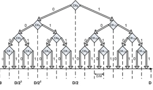
Fig. 2. Decision tree for the x dimension: label 0 coming out of a classification node cxi means “not belong to cxi”, while label 1 means
otherwise. In this example,m=4.
• M horizontal regions, called y-regions,{ry0,r1y, ..,ryM−1}
where each regionry
i is the rectangle containing all points with y-coordinate y ∈[iD/M,(i+ 1)D/M]
Our goal is to predict which x-region rx
i and y-region riy that each sensor S belongs to. We then simply use the center point of the cell[iD/M,(i+1)D/M]×[jD/M,(j+1)D/M]
as the estimated position of node S. The parameter M (or m) controls how close we want to localize a sensor. If the above prediction is indeed correct, the location error for node S is at most D/(M√2). However, every SVM is subject to some classification error, and so we should maximize the probability that S is classified into its true cell, and, in case of misclassification, minimize the localization error.
C. Classification Strategies
A component of SVM is to define the target classes for classification. We propose two strategies for this purpose: the multi-class strategy (MCS) and the decision-tree strategy (DTS). They are presented in the following subsections.
1) Multi-class strategy (MTS): We define the following2M
classes:
• M classes for the x dimension {cx0, cx1, ..., cxM−1}:
Each class cxi contains nodes with the x-coordinate ∈
[iD/M,(i+ 1)D/M].
• M classes for the y dimension {cy0, cy1, ..., cyM−1}:
Each class cyi contains nodes with the y-coordinate ∈
[iD/M,(i+ 1)D/M].
Obviously, each class represents a geographic region rx i (or riy) defined earlier. Consider a sensor node S. We formulate the problem of estimating its x-coordinate as a multi-class SVM classification, where the number of classes isM. Multi-class SVM is a generalized version of the traditional SVM, or binary SVM, where the number of classes is 2. Many algorithms have been proposed for multi-class SVM. The most popular methods are (see overview in [22]): the “one vs. one” algorithm, the “one vs. all” algorithm, and the “DAGSVM” algorithm. We can use any of these algorithms. Supposing that nodeS is classed into the x-classcxiand the y-classcyi, its estimate location is[(i+ 1/2)D/M,(j+ 1/2)D/M].
2) Decision-tree strategy (DTS): The multi-class strategy
typically involves M(M −1)/2 binary SVM classifications for each dimension. The decision-tree strategy proposed below uses only M −1 binary classifications in the training phase and log2M binary classifications in the decision phase. We define the following2M−2 classes (whereM = 2m):
• M−1classes for thexdimension{cx1, cx2, ..., cxM−1}:
Each class cxi contains nodes with the x-coordinate greater or equal toiD/M.
• M−1classes for theydimension{cy1, cy2, ..., cyM−1}:
Each class cyi contains nodes with the y-coordinate greater or equal toiD/M.
Firstly, we train on these2M−2 classes separately based on binary SVM classification. Then, we organize the classifiers for each dimension into a binary decision tree. Let us focus on the x-dimension, whose decision tree is illustrated in Figure 2. Each tree node is an x-class and the two outgoing links represent the outcomes (0: “not belong”, 1: “belong”) of classification on this class. The classes are assigned to the tree nodes such that if we traverse the tree in the order{leftchild
→parrent→rightchild}, the result is the ordered listcx1 →
cx2→...→cxM. Given this decision tree, each sensorS can estimate its x-coordinate using the following algorithm:
Algorithm 3.1 (X-dimension Localization): Estimate the
x-coordinate of sensorS:
1) i =M/2 (start at root of the treecxM/2) 2) IF (SVM predictsS not in class cxi)
a) IF (cxi is a leaf node) RETURN x(S) =
(i−1/2)D/M
b) ELSE Move to leftchildcxj and set i=j 3) ELSE
a) IF (cxi is a leaf node) RETURN x(S) =
(i+1/2)D/M
b) ELSE Move to rightchildcxtand set i=t 4) GOTO Step 2)
Similarly, a decision tree is built for the y-dimension classes and each sensorS estimates its y-coordinatey(S) based on
the y-dimension localization algorithm (like Algorithm 3.1).
The estimated location for node S, consequently, is (x(S),
y(S)). Using these algorithms, localization of a node requires
visitinglog2M classifiers of each decision tree, after each visit the geographic range that contains node S downsizing by a half. Table I provides a comparison between the multi-class and decision tree strategies in terms of the number of binary classifications involved in the training phase, testing phase, and the amount of SVM model information (counted for both x- and y-dimensions).
D. Network protocols
We recall that the information that a node S needs to localize itself is consisted of the following (according to Formula 4):
• The support vectors{Si:(i,yi,α∗i)}andb∗for each class
• The hop-count distance from each beacon node toS, so
TABLE I
MULTI-CLASS STRATEGY VS.DECISION-TREE STRATEGY: TRAINING
TIME,TESTING TIME,AND AMOUNT OFSVMMODEL INFORMATION
Strategy Training Testing #SVM models
MCS/One vs. one M(M−1) M(M−1) M(M−1)
MCS/One vs. all 2M 2M 2M
MCS/DAGSVM M(M−1) 2log2M(M2+1) M(M−1)
DTS 2M−2 2log2M 2M−2
TABLE II
NETWORK CONNECTIVITY SUMMARY
Radius Min degree Max degree Avg degree Netw. Diameter
r=7m 2 27 14 25 (hops)
r=10m 8 48 28 16 (hops)
Who computes those values and how are they communi-cated to node S? We divide the entire process into 3 phases: training phase, advertisement phase, and localization phase.
1) Training Phase: We assume that a beacon is selected
as the head beacon. The head beacon will later run the SVM training algorithm and therefore should be the most resourceful node. This is a feasible assumption because the head node can be a base station or sink node of the sensor network. The training phase is conducted among the beacon nodes. Firstly, each beacon node sends a HELLO message to every other beacon node. After this round, a beacon knows its hop-count distance from each other beacon node. Next, each beacon node sends an INFO message to the head beacon, containing the location of the sending node and its pairwise hop-count distances from the other beacon nodes. After this round, the head beacon knows the location of every beacon and hop-count distance between every two beacons. The head beacon then runs the SVM training procedure using either the multi-class strategy or the decision-tree strategy. As a result, we obtain the SVM model information that will be disseminated to every node in the network.
2) Advertisement Phase: The head beacon broadcasts the
SVM model information to all the sensors in the network. Therefore, each node S possesses all the information needed to compute hK(S) in Formula 4, except for the hop-count distance h(S, Si) to each beacon node Si. For this purpose, each beacon node, except for the head beacon, broadcasts a HELLO message to the entire network, so that upon receipt of this HELLO message, each node can obtain the hop-count distance to the beacon.
3) Localization Phase: After receiving the SVM model
information from the advertisement phase, each non-beacon node follows the x-dimension localization and y-dimension localization algorithms (see Algorithm 3.1) to estimate its location (x(S),y(S)).
IV. SIMULATIONSTUDY
We conducted a simulation study to assess the location accuracy of our approach. A network of 1000 sensors located in a 100m × 100m 2-D area was simulated, where uniform random distribution is used for generating sensor locations
and the beacon sensors. We compared the multi-class strategy (MCS) and decision-tree strategy (DTS) together under the effects of beacon population, network density, and the border problem. We considered two levels of network density, 7m and 10m communication ranges, summarized in Table II, and three different beacon populations: 5% of the network size (k = 50 beacons), 15% (k = 150 beacons), and 25%
(k = 250 beacons). We used the libsvm [21] software for
SVM classification. For the multi-class strategy, we employ the one vs. one method as recommended by [21], [22]. The γ parameter in Equation 5 and C parameter in Inequality 3 were automatically determined by the mechanisms oflibsvm. We set m= 7 (i.e.,M = 128) throughout the study.
Figures 3 and 4 plot the average, max, and standard devia-tion of locadevia-tion errors for the 10m network and range-7m network. It is observed that DTS always provides better results than MCS. When only 5% of the network serve as beacons, DTS’s localization error is 6m on average while that of MCS is 11m (almost double). The main reason is probably because DTS uses a lot fewer binary SVM classifications than MCS, thus resulting in smaller accumulative error after the entire prediction process ends. The gap between these two strategies is narrowed down as more nodes serve as beacons. Regarding the beacon population size, it is understandable that when this population is larger, the localization gets more accurate. Both strategies provide good results when 25% of the network serve as beacons, in which case the error is about 2-3m and no more than 15m. The standard deviation is also small (about 2m), which implies that most sensors’ locations are very well estimated.
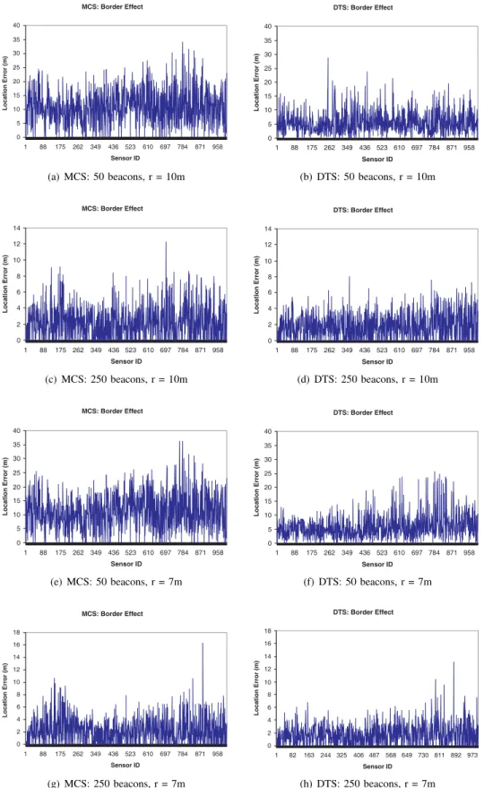
Often occurring in many existing localization techniques is the border problem, in which border sensors are usually positioned with larger error than sensors inside thefield. Figure 5 plots the location errors of all sensors in the network sorted in the order of sensors close to the center of thefieldfirst and sensors near the edge last. If the border problem exists, we should see an up-hill curve pattern from the left to the right side of the graph. However, this pattern is rarely seen in this
figure; the majority of errors have similar values, implying that the border problem is well-addressed in our proposed approach. This desirable property is understandable. Because the location of each sensor is estimated only based on distances to the beacons and independently of other sensors, whether a sensor is near the border of lies inside should not have a big impact on the location error.
V. CONCLUSION
We have presented an approach based on the concept of SVM to localize nodes in a large-scale sensor networks. In our SVM model, the beacon nodes serve as the training points and the kernel function uses only mere connectivity information. Therefore, the proposed approach can be used for networks that do not require expensive ranging and spe-cialized (and/or mobile) devices. It can be realized using two alternative strategies: the multi-class strategy (MCS) and the decision-tree strategy (DTS). Our simulation study have shown
Communication range 10m 0 2 4 6 8 10 12 5% 15% 25%
Beacon population (% network size)
Avg. Location Error (m)
MCS-r10 DTS-r10
(a) Average location error
Communication range 10m 0 5 10 15 20 25 30 35 40 5% 15% 25%
Beacon population (% network size)
Max Location Error (m)
MCS-r10 DTS-r10
(b) Max location error
Communication range 10m 0 1 2 3 4 5 6 7 5% 15% 25%
Beacon population (% network size)
Location Error Std. Dev. (m)
MCS-r10 DTS-r10
(c) Standard deviation Fig. 3. MCS vs. DTS (communication range 10m): Statistics on location error of each technique under different beacon populations.
Communication range 7m 0 2 4 6 8 10 12 5% 15% 25%
Beacon population (% network size)
Avg. Location Error (m)
MCS-r7 DTS-r7
(a) Average location error
Communication range 7m 0 5 10 15 20 25 30 35 40 5% 15% 25%
Beacon population (% network size)
Max Location Error (m)
MCS-r7 DTS-r7
(b) Max location error
Communication range 7m 0 1 2 3 4 5 6 7 5% 15% 25%
Beacon population (% network size)
Location Error Std. Dev. (m)
MCS-r7 DTS-r7
(c) Standard deviation Fig. 4. MCS vs. DTS (communication range 7m): Statistics on location error of each technique under different beacon populations.
that both MCS and DTS provide good localization accuracy and alleviate the border problem effectively. We, however, recommend DTS because of his superior performance over MCS. Our future research includes a comparison between DTS with other existing localization techniques as well as its performance in networks with coverage holes. We also plan a prototype implementation of DTS.
REFERENCES
[1] L. Doherty, L. E. Ghaoui, and K. S. J. Pister, “Convex position estimation in wireless sensor networks,” inIEEE Infocom, April 2001. [2] Shang, Juml, Zhang, and Fromherz, “Localization from mere
connec-tivity,” inACM Mobihoc, 2003.
[3] C. Savarese, J. Rabaey, and J. Beutel, “Locationing in distributed ad-hoc wireless sensor networks,” inIEEE International Conference on Acoustics, Speech, and Signal Processing, Salt Lake city, UT, 2001. [4] N. B. Priyantha, H. Balakrishnan, E. Demaine, and S. Teller,
“Anchor-free distributed localization in sensor networks,” inACM Sensys, 2003. [5] S. Capkun, M. Hamdi, and J.-P. Hubauz, “Gps-free positioning in mobile ad hoc networks,” inHawai International Conference on System Sciences, 2001.
[6] L. Meertens and S. Fitzpatrick, “The distributed construction of a global coordinate system in a network of static computational nodes from inter-node didstances,” Kestrel Institute, Tech. Rep., 2004.
[7] D. Moore, J. Leonard, D. Rus, and S. Teller, “Robust distributed network localization with noisy range measurements,” inACM Sensys, Baltimore, MA, November 2004.
[8] D. Niculescu and B. Nath, “Ad hoc positioning system (aps),” inIEEE Globecom, 2001.
[9] N. Bulusu, V. Bychkovskiy, D. Estrin, and J. Heidemann, “Scalable ad hoc deployable rf-based localization,” inGrace Hopper Celebration of Women in Computing Conference, Vancouver, Canada, October 2002.
[10] A. Savvides, H. Park, and M. Srivastava, “The bits andflops of the n-hop multilateration primitive for node localization problems,” inWorkshop on Wireless Networks and Applications (in conjunction with Mobicom 2002), Atlanta, GA, September 2002.
[11] A. Savvides, C.-C. Han, and M. B. Strivastava, “Dynamicfine-grained localization in ad hoc networks of sensors,” in ACM International Conference on Mobile Computing and Networking (Mobicom), Rome, Italy, July 2001, pp. 166–179.
[12] S. Simic and S. S. Sastry, “Distributed localization in wireless ad hoc networks,” University of California at Berkeley, Tech. Rep., 2002. [13] C. Whitehouse, “The design of calamari: an ad hoc localization
sys-tem for sensor networks,” Master’s thesis, University of California at Berkeley, 2002.
[14] D. Niculescu and B. Nath, “Ad hoc positioning system (aps) using aoa,”
inIEEE Infocom, 2003.
[15] R. Nagpal, H. Shrobe, and J. Bachrach, “Organizing a global coordinate system from local information on an ad hoc sensor network,” in International Symposium on Information Processing in Sensor Networks, 2003.
[16] T. He, C. Huang, B. Blum, J. Stankovic, and T. Abdelzaher, “Range-free localization schemes in large scale sensor networks,” inACM Conference on Mobile Computing and Networking, 2003.
[17] R. Stoleru, J. A. Stankovic, and D. Luebke, “A high-accuracy, low-cost localization system for wireless sensor networks,” inACM Sensys, San Diego, CA, November 2005.
[18] N. B. Priyantha, H. Balakrishnan, E. Demaine, and S. Teller, “Mobile-Assisted Localization in Wireless Sensor Networks,” in IEEE INFO-COM, Miami, FL, March 2005.
[19] X. Nguyen, M. Jordan, and B. Sinopoli, “A kernel-based learning approach to ad hoc sensor network localization,” IEEE Transactions on Sensor Networks, vol. 1, pp. 134–152, 2005.
[20] V. N. Vapnik,Statistical Learning Theory. Wiley-Interscience, 1998. [21] C.-C. Chang and C.-J. Lin, LIBSVM – A library for Support
Vector Machines, National Taiwan University. [Online]. Available: http://www.csie.ntu.edu.tw/ cjlin/libsvm
MCS: Border Effect 0 5 10 15 20 25 30 35 40 1 88 175 262 349 436 523 610 697 784 871 958 Sensor ID Location Error (m) (a) MCS: 50 beacons, r = 10m DTS: Border Effect 0 5 10 15 20 25 30 35 40 1 88 175 262 349 436 523 610 697 784 871 958 Sensor ID Location Error (m) (b) DTS: 50 beacons, r = 10m MCS: Border Effect 0 2 4 6 8 10 12 14 1 88 175 262 349 436 523 610 697 784 871 958 Sensor ID Location Error (m) (c) MCS: 250 beacons, r = 10m DTS: Border Effect 0 2 4 6 8 10 12 14 1 88 175 262 349 436 523 610 697 784 871 958 Sensor ID Location Error (m) (d) DTS: 250 beacons, r = 10m MCS: Border Effect 0 5 10 15 20 25 30 35 40 1 88 175 262 349 436 523 610 697 784 871 958 Sensor ID Location Error (m) (e) MCS: 50 beacons, r = 7m DTS: Border Effect 0 5 10 15 20 25 30 35 40 1 88 175 262 349 436 523 610 697 784 871 958 Sensor ID Location Error (m) (f) DTS: 50 beacons, r = 7m MCS: Border Effect 0 2 4 6 8 10 12 14 16 18 1 88 175 262 349 436 523 610 697 784 871 958 Sensor ID Location Error (m) (g) MCS: 250 beacons, r = 7m DTS: Border Effect 0 2 4 6 8 10 12 14 16 18 1 82 163 244 325 406 487 568 649 730 811 892 973 Sensor ID Location Error (m) (h) DTS: 250 beacons, r = 7m
Fig. 5. The border problem: Location error for every sensor, sorted in the order of nodes near the center of thefieldfirst and nodes near the edge last.
[22] C.-W. Hsu and C.-J. Lin, “A comparison of methods for multi-class