Optimal jackknife for unit root models

Singapore Management University

Institutional Knowledge at Singapore Management University

Research Collection School Of Economics

School of Economics

4-2015

Optimal jackknife for unit root models

Ye CHEN

Capital University of Economics and Business

Jun YU

Singapore Management University, [email protected]

DOI:

https://doi.org/10.1016/j.spl.2014.12.014

Follow this and additional works at:

https://ink.library.smu.edu.sg/soe_research

Part of the

Econometrics Commons

This Journal Article is brought to you for free and open access by the School of Economics at Institutional Knowledge at Singapore Management University. It has been accepted for inclusion in Research Collection School Of Economics by an authorized administrator of Institutional Knowledge at Singapore Management University. For more information, please [email protected].

Citation

CHEN, Ye and Jun YU. Optimal jackknife for unit root models. (2015).Statistics and Probability Letters. 99, 135-142. Research Collection School Of Economics.

Optimal Jackknife for Unit Root Models

∗

Ye Chen and Jun Yu

Singapore Management University

October 19, 2014

Abstract

A new jackknife method is introduced to remove the first order bias in the discrete time and the continuous time unit root models. It is optimal in the sense that it minimizes the variance among all the jackknife estimators of the form considered in Phillips and Yu (2005) and Chambers and Kyriacou (2013). Simulations show that the new jackknife reduces the variance of that of Chambers and Kyriacou by about 10%. The results continue to hold true in near unit root models.

Keywords: Bias reduction, Variance reduction, Vasicek model, Autoregression

1

Introduction

Many estimators suffer from finite sample bias in dynamic models. Subsampling methods have been found useful to reduce the bias. The jackknifing method of Quenouille (1949) is widely used approaches to achieve this. The basic idea of this method is to use a subsampling technique to estimate the bias, and then to subtract the bias estimate from the initial (biased) estimator. The bias estimate is formed through linear combinations of full sample estimate and subsample estimates. Under mild conditions, the jackknife estimator can remove the first order bias.

The bootstrap method of Efron (1979) generalizes the jackknife for bias reduction. It was subse-quently found that the bootstrap was more effective in reducing the bias than the jackknife; see for example, Hall (1992) and Shao and Tu (1995) for more detailed discussions. Nevertheless, the jack-knife remains appealing for its ease in implementation. In addition, it is computationally not much more expensive than the initial estimator. Moreover, it is often found that the jackknife continues to reduce the bias when the error distribution is misspecified; see for example, Phillips and Yu (2005, PY hereafter).

In the context of a discrete time unit root model, Chambers and Kyriacou (2013, CK hereafter) pointed out that the jackknife of PY cannot completely remove the first order bias. A revised jackknife was proposed in CK and was shown to perform better than the PY estimator for bias reduction. While

the jackknife of CK reduces the bias of the original estimator, it always increases the variance, as is the case with other jackknife estimators. The increased variance is due to the use of weighted average of the bias estimates. However, the variance can be reduced by choosing weights carefully.

In this paper, we propose an improved jackknife estimator for unit root models. Our estimator is optimal in the sense that it not only removes the first order bias, but also minimizes the variance. Hence, it has better finite sample properties than the CK estimator. Unlike the estimators of CK, the weights are not the same across different subsamples. Optimal weights are derived and the finite sample performance of the new estimator is examined for both the discrete time and the continuous time unit root models. It is found that the optimal jackknife estimator offers about 10% reduction in variance over the CK estimator without compromising bias reduction. When the root is not exactly one but close to one, we provide evidence that our optimal jackknife continues to work well.

Let the parameter of interest by β or κ. Let eθj denotes the LS/ML estimator of θ from the

jth subsample of sample length l (i.e., m×l = n), θeP Y, θeCK, θeCY the jackknife estimators of PY, CK, and the present paper, respectively. Following CK, we define Z =R1

0 W dW/ R1 0 W 2_{, Z} j = Rj/m (j−1)/mW dW/ Rj/m (j−1)/mW

2_{, whereWis a standard Brownian motion, andµ=E(Z) andµ}

j=E(Zj).

2

Optimal Jackknife for Unit Root Models

2.1

Jackknife methods of PY and CK

Considering a simple unit root model with initial value y0=Op(1):

yt=βyt−1+εt, εt∼iid(0, σ2ε), t= 1, . . . , n, withβ = 1. (2.1)

With the available data {yt}nt=0, the LS estimator of β is βe= Pn

t=1yt−1yt/P n

t=1yt2−1. When εt is

normally distributed,βeis also the ML estimator ofβ, conditional ony0.

Following the original work of Quenouille (1949), PY (2005) utilized the subsample estimators of

β to achieve bias reduction with the following formula:

e β_mP Y = m m−1βe− 1 m−1   1 m m X j=1 e βj  =βe− 1 m−1   1 m m X j=1 e βj−βe  , (2.2)

whereβeis the LS/ML estimator ofβbased on the full sample, i.e.,y1, . . . , yn;βejis the LS/ML estimator

ofβ based on thejth subsample, i.e.,y(j−1)l+1, . . . , yjl. To check the validity of this jackknife method,

consider the following Nagar approximation:

Eβe =β+b1 n +o n −1 , Eβej =β+b1 l +o l −1 , (2.3)

which can be derived from a set of mild conditions, asn, l→ ∞. Substituting (2.3) into (2.2), we have

Eβe_mP Y

=β+o n−1

method of PY estimates the bias in the initial estimator βe by _m1₋₁ 1 m Pm j=1βej−βe . Particularly effective bias reduction can be achieved by choosingm= 2 and the estimator becomes:

e βP Y = 2βe− 1 2 e β1+βe2 . (2.4)

Both PY and Chambers (2013) have reported evidence to support this method for the purpose of bias reduction in different contexts.

The Nagar approximation is a general result and may be verified by Sargan’s (1976) theorem. Given the mild conditions under which Sargan’s theorem holds, it is rather surprising that the standard jack-knife fails to remove the first order bias in the unit root model. This failure was first documented in CK (2013). The basic argument of CK is that in (2.3), b1 is not constant any more in the unit root model. Instead, it depends on the initial condition. As the initial condition varies across different sub-samples, the jackknife cannot eliminate the first order bias term. Specifically, the limiting distribution ofl(βej−1) is Rj/m (j−1)/mW dW/ mRj/m (j−1)/mW

2_{whose expectation depends onj. To eliminate the first} order asymptotic bias, CK proposed the following modified jackknife estimator:

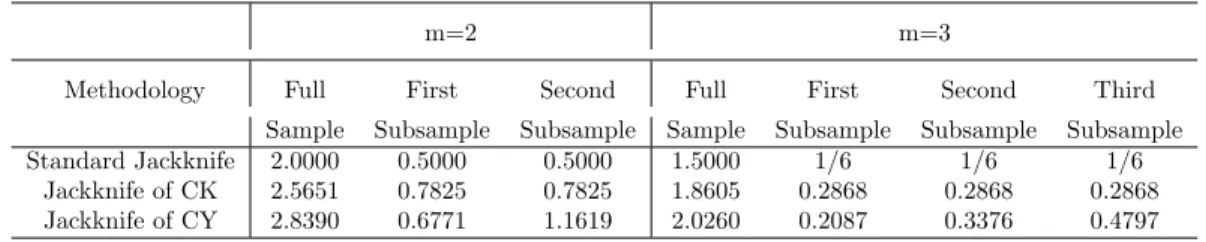
e β_mCK =bCK_m βe−δCK_m m X j=1 e βj, (2.5) where bCK_m = Pm j=1µj Pm j=1µj−µ , δ_mCK = µ mPm j=1µj−µ . (2.6) Whenµ1 =· · · =µm=µ, bCKm =m/(m−1) = bP Ym , and δCKm = 1/ m2−m . Under model (2.1), CK showed that µ=µ1 =−1.7814, µ2 =−1.1382, µ3 =−0.9319,µ4 = −0.8143, etc. That is, the bias becomes smaller and smaller as we go deeper and deeper into subsampling. Substituting these expected values into the formula (2.6), we can calculate the weights. Table 1 reports the weights when

m= 2 andm= 3. We also report the weights of PY for comparison. Asµ2 is closer to zero than µ1 andµ, a larger weight is assigned to the full sample estimator, compared to the PY estimator. Among all possible values ofm, CK proposed to choosemto minimize the root mean squared errors (RMSE). Being the optimal method, our jackknife method always offers an improvement to CK even when the optimalmis used.

2.2

Optimal jackknife

The jackknife estimator of CK increases the variance, compared to the LS/ML estimator. In this paper, we introduce a new jackknife estimator, which can remove the first order bias and minimize the variance for any given m. To do so, we select the weights, bCY

Table 1: Weights assigned to the full- and sub-sample estimators for alternative jackknife methods

m=2 m=3

Methodology Full First Second Full First Second Third

Sample Subsample Subsample Sample Subsample Subsample Subsample

Standard Jackknife 2.0000 0.5000 0.5000 1.5000 1/6 1/6 1/6

Jackknife of CK 2.5651 0.7825 0.7825 1.8605 0.2868 0.2868 0.2868

Jackknife of CY 2.8390 0.6771 1.1619 2.0260 0.2087 0.3376 0.4797

variance of the new jackknife estimator defined byβe_mCY =bCY_m βe−P

m j=1a CY j,mβej, i.e., min bCY m ,{aCYj,m}mj=1 V arβe_mCY , (2.7)

subject to two constraints:

bCY_m = m X j=1 aCY_j,m+ 1, (2.8) bCY_m µ = m m X j=1 aCY_j,mµj, (2.9)

whereµ=µ1. These two constraints are used to ensure the first order bias is fully removed. The first order conditions with respect toaCY_j,m are:

0 = bCY_m 2m(µ−µj) (m−1)µ V ar(βe)−2 µ−mµj (m−1)µCov(β,e βe1)−2Cov(β,e βej) +aCY_1,m× 2µ−mµj (m−1)µV ar(βe1)−2 m(µ−µj) (m−1)µ Cov(β,e βe1) + 2Cov(β,e βej) +· · ·+ m X i=2 aCY_i,m× −2m(µ−µi) (m−1)µCov(β,e βei) + 2 µ−mµi (m−1)µCov(βe1,βei) + 2Cov(βei,βej) , (2.10)

forj= 2,· · ·, m. In addition, we have:

bCY_m = aCY_2,mm(µ−µ2) (m−1)µ +· · ·+ a CY m,m m(µ−µm) (m−1)µ + m m−1, aCY_1,m = aCY_2,mµ−mµ2 (m−1)µ+· · ·+a CY m,m µ−mµm (m−1)µ + 1 m−1.

To eliminate the first order bias, one must first obtain µ, µ2, . . . , µm, as CK did. To minimize the

variance of the new estimator, one must calculate the exact variances and covariances of the finite sample distributions. However, it is known in the literature that the exact moments are difficult to obtain analytically in dynamic models. To simplify the derivations, we propose to approximate the

moments of the finite sample distributions by those of the limit distributions, but will check the quality of these approximations in simulations.

The variances can be computed by combining the techniques of White (1961) and CK. Note that:

n2V ar(βe) =E R1 0 W dW R1 0 W2 !2 −µ2+o(1).

Similarly, the variance of the subsample estimators is:

l2V ar(βej) =E   Rj/m (j−1)/mW dW mRj/m (j−1)/mW 2   2 −µ2j+o(1), j= 1,2, . . . , m.

Let N(a, b) = R_abW dW, D(a, b) = R_abW2 (0 ₆ a < b ₆ 1), and Ma,b(θ1, θ2) denote the joint moment generating function (MGF) of N(a, b) and D(a, b). Following Magnus (1986), we use the following expression in numerical integrations:

E N(a, b) D(a, b) 2 = Z ∞ 0 θ2 ∂2Ma,b(θ1,−θ2) ∂θ2 1 |θ1=0 dθ2.

With the expression forMa,b(θ1, θ2) from CK, we have the approximate variance for the full sample estimator and subsample estimators in the discrete time unit root model:

n2V ar(βe) = l2V ar(βe1) = 10.1123 +O(n−1).

l2V ar(βe2) = 5.3612 +O(n−1).

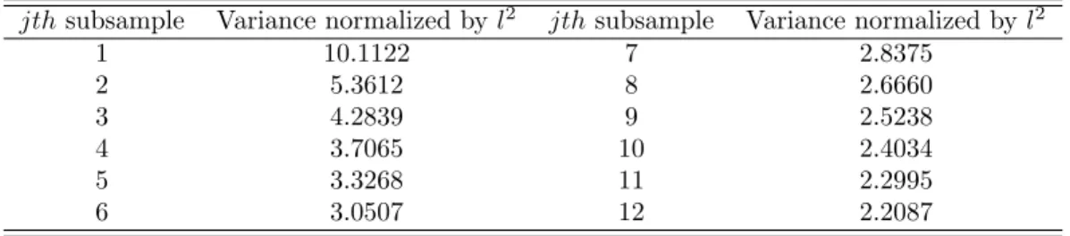
Table 2 lists the variances of all the subsample estimators for m = 1, . . . ,12. It can be seen that the variance of the subsample estimator decreases asjincreases. The largest difference occurs between

j = 1 andj = 2. Ifmis allowed to go to infinity, the limit distribution of the jackknife converges to that of the LS, as pointed out by CK.

Table 2: Variances of subsample estimators

jthsubsample Variance normalized byl2 jthsubsample Variance normalized byl2

1 10.1122 7 2.8375 2 5.3612 8 2.6660 3 4.2839 9 2.5238 4 3.7065 10 2.4034 5 3.3268 11 2.2995 6 3.0507 12 2.2087

To calculate the covariances, we note that: n2Cov(β,e βej) =E   R1 0 W dW R1 0 W 2 Rj/m (j−1)/mW dW Rj/m (j−1)/mW 2  −mµµj+O(n−1),16j6m. n2Cov(βei,βej) =E   Ri/m (i−1)/mW dW Ri/m (i−1)/mW 2 Rj/m (j−1)/mW dW Rj/m (j−1)/mW 2  −m2µiµj+O(n−1),16i < j6m.

Hence, we need to compute the covariance between the limit distribution of the full sample estimator and that of any subsample estimator, and the covariance between any two subsample limit distributions. The following lemma and proposition obtain the expression for the MGF of the covariances.

Lemma 2.1 Let Ma,b,c,d(θ1, θ2, ϕ1, ϕ2)denote the MGF ofN(a, b),N(c, d),D(a, b)andD(c, d)with (0₆a < b₆1) and(0₆c < d₆1). Then the expectation of N_D(_(a,ba,b)₎N_D(₍c,d_c,d)) is given by:

E _{N(a, b)} D(a, b) N(c, d) D(c, d) = Z ∞ 0 Z ∞ 0 ∂2_M a,b,c,d(θ1,−θ2, ϕ1,−ϕ2) ∂θ1∂ϕ1 |θ1=0,ϕ1=0dθ2dϕ2. (2.11)

The following proposition obtains the expression for the MGF of N(a, b), N(c, d), D(a, b) and

D(c, d), and the covariances.

Proposition 2.2 The MGF M0,a,b,1(θ1, θ2, ϕ1, ϕ2)is given by

M0,a,b,1(θ1, θ2, ϕ1, ϕ2) = exp _aλ−θ 1−sϕ1 2 [1−(2p+η−λ)$2]−1/2× cosh(eλ)−θ1 λ sinh(eλ) −1/2 cosh(sη)−(θ1−λ)κb+ϕ1+λ η sinh(sη) −1/2 , (2.12) withe= 1−b,s=b−a,ξ=λ=√−2θ2,η= √ −2θ2−2ϕ2,$2b = exp(2λe)−1 2λ ,κb= 1−(θ1−λ)$2b −1 exp (2λe), $a2= exp(2ηs)−1 2η ,κa= exp(2ηs) 1−[ϕ1+(θ1−λ)κb+(λ−η)]$2a,p= [ϕ1+(θ1−λ)κb+(λ−η)]κa−ϕ1 2 , and$ 2₌ exp(2aλ)−1 2λ .

The MGF Ma,b,c,d(θ1, θ2, ϕ1, ϕ2) is given by

Ma,b,c,d(θ1, θ2, ϕ1, ϕ2) = exp( −eϕ1−sθ1 2 ){1−a[(2p+θ1−η)κa−θ1+η]} −1/2 × [1−(c−b)(ϕ1−λ) (κc−1)]− 1/2h cosh(eλ)−ϕ1 λ sinh(eλ) i−1/2 cosh(sη)−2p+θ1 η sinh(sη) −1/2 , with e=d−c,s=b−a,$2 c = exp(2eλ)−1 2λ , $ 2 a = exp(2ηs)−1 2η , κa = 1−(2p+θ1−η)$a2 −1 exp (2ηs), κc=1−(ϕ1−λ)$2c −1

exp(2eλ)andp= (ϕ1−λ)(κc−1)

2[1−(c−b)(ϕ1−λ)(κc−1)].

Chen and Yu (2011) gives the expression of the second derivative of the MGFM0,a,b,1(θ1, θ2, ϕ1, ϕ2) andMa,b,c,d(θ1, θ2, ϕ1, ϕ2), which is used to compute the numerical value of covariance. Whenm= 2,

we have following approximate covariances between the full sample estimator and the two subsample estimators:

n2Cov(β,e βe1) = 10.0376 +O(n−1); (2.13)

n2Cov(β,e βe2) = 11.5863 +O(n−1); (2.14)

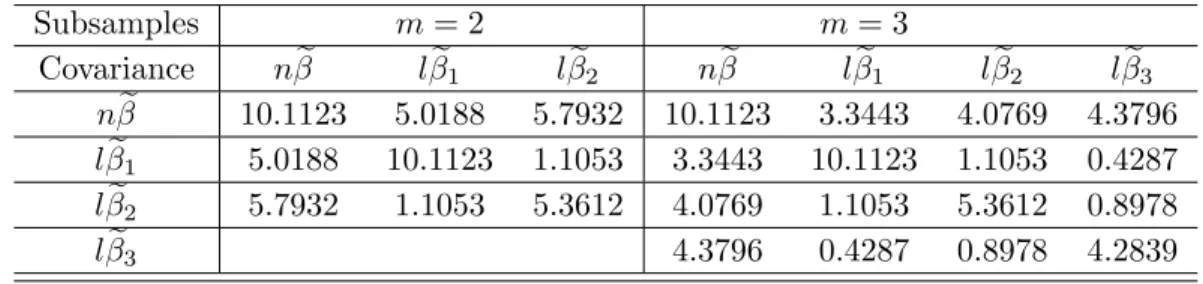
n2Cov(βe1,βe2) = 4.4212 +O(n−1). (2.15) There are several interesting findings here. First, the covariances between the full sample estimator and the second subsample estimator are similar to, but slightly larger than that between the full sample estimator and the first subsample estimator, although the variance of the second subsample estimator is smaller. This is because the correlation between the full sample estimator and the second subsample estimator is larger due to the increased order of magnitude of the initial condition. Second, these two covariances are much larger than the covariance between the two subsample estimators. This is not surprising as the data used in the two subsamples estimators do not overlap.

Table 3: Approximate variances and covariances for the full sample and subsamples whenm= 2,3

Subsamples

m

= 2

m

= 3

Covariance

n

β

e

l

β

e

l

β

e

n

β

e

l

β

e

l

β

e

l

β

e

n

β

e

10.1123

5.0188

5.7932

10.1123

3.3443

4.0769

4.3796

l

β

e

5.0188

10.1123

1.1053

3.3443

10.1123

1.1053

0.4287

l

β

e

5.7932

1.1053

5.3612

4.0769

1.1053

5.3612

0.8978

l

β

e

4.3796

0.4287

0.8978

4.2839

Table 3 summarizes the approximate values of the variances and covariances whenm= 2,3. Given the values of variances and covariances, we further compute the optimal jackknife estimator when

m= 2:

e

β_{J K}CY = 2.8390βe−(0.6771βe1+ 1.1619βe2). (2.16) and the optimal jackknife estimator whenm= 3:

e

β_{J K}CY = 2.0260βe−(0.2087βe1+ 0.3376βe2+ 0.4797βe3). (2.17) It can be easily shown that the above results are applicable to a continuous time unit root model. Although it was proven recently in Bao,Ullah and Zinde-Walsh (2013) that the exact moment may not exist, the moment we try to approximate can be understood as the pseudo moment.

Considering the following Vasicek model with y0= 0:

The parameter of interest here is κthat captures the persistence of the process. The observed data are assumed to be recorded discretely at (h,2h,· · ·, nh(= T)) in the time interval (0, T]. So h is the sample interval,n is the total number of observations and T is the time span. The bias formula for κ_e is similar to that for βe in (2.1). However, the direction of the bias is opposite and the bias depends on T, not n; see Yu (2012). If T → ∞, the so-called long span limit distribution of _eκ is given by T(_eκ−1) ⇒ −R1

0 W dW/

R1

0 W

2_{. Similarly, the long span limit distributions of the} sub-sample estimators are T(_eκj−1)⇒ −R

j/m

(j−1)/mW dW/T

Rj/m

(j−1)/mW

2_{, forj = 1, . . . , m. Obviously, the} only difference between these limit distributions and those in the discrete time model is the minus sign. Hence, the variances and covariances of the two sets of limit distributions are the same but the expectations change the sign. Consequently, the optimal jackknife estimator remains unchanged.

3

Simulation Studies

First, we simulate data from Model (2.1) and evaluate the performance of alternative jackknife methods by applying them to five different sample sizes, i.e. n= 12,24,48,96,108. It is reasonable to consider the small sample sizes since we focus on the finite sample property. We compare three methods, namely, the CK jackknife method based on weights from Table 1, the CY jackknife method based on (2.16) and (2.17) where the weights are derived from the approximate variances and covariances, the CY jackknife method where the weights are calculated from the exact variances and covariances obtained from the finite sample distributions when m = 2 and m = 3. It is important to measure the efficiency gain of the proposed method by ratio of the variances. Moreover, the weights are obtained based on the variances and the covariances of the limit distributions but not on the finite sample distributions. Hence, it is informative to examine the importance of the approximation error. Although it is difficult to obtain the analytical expressions for the variances and the covariances of the finite sample distribution, they can be computed using simulated data in a Monte Carlo study, provided the number of replications is large enough. In this paper, we always set the number of replications at 5,000. The results are reported in Table 4 where for each case, we calculate the mean, the variance and the RMSE for the estimates ofβ.

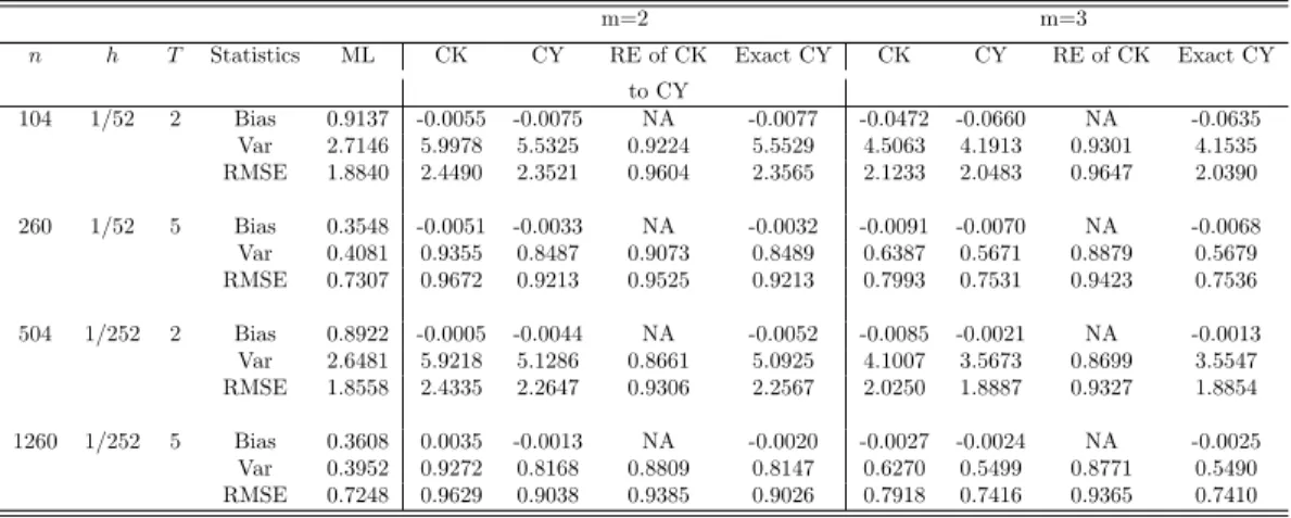
Second, we simulate data from Model (2.18) and employ the three jackknife methods to estimateκ. Table 6 shows the results based on two sampling intervalsh= 1/52,1/252, corresponding to the weekly and daily frequency. The time span, T, is set at 2 years and 5 years. These settings are empirically realistic for modeling interest rates and volatility.

The simulation results obtained above are based on the assumption that the true model has a unit root. In practice, however, the persistence parameter is often unknown and has to be estimated. Based on the estimator of slope coefficient, it is not easy to tell whether the true value is one or not. To check the robustness of our results in the persistent case, we now compare the finite sample performance with three jackknife estimators in the context of the discrete time AR model, with a root that is local to unity.

Table 4: Finite sample performance of alternative jackknife estimators for the discrete time unit root model whenm= 2,3, where RE means the relative efficiency.

m=2 m=3

n Statistics ML CK CY RE of CK Exact CY CK CY RE of CK Exact CY

to CY to CY 12 Bias -0.1282 -0.0637 -0.0665 -0.0671 -0.0985 -0.0998 -0.0987 100*Var 5.6654 17.9035 16.1215 0.9005 16.0528 27.2300 20.2931 0.7452 16.6729 10*RMSE 2.7035 4.2789 4.0698 0.9511 4.0624 5.3103 4.6139 0.8689 4.2009 36 Bias -0.0464 -0.0073 -0.0078 -0.0079 -0.0084 -0.0093 -0.0096 100*Var 0.7029 1.5185 1.3181 0.8680 1.3061 1.0708 0.9503 0.8874 0.9465 10*RMSE 0.9581 1.2344 1.1507 0.9322 1.1456 1.0382 0.9792 0.9432 0.9776 48 Bias -0.0360 -0.0064 -0.0062 -0.0062 -0.0059 -0.0061 -0.0061 100*Var 0.4061 0.8648 0.7570 0.8753 0.7534 0.6029 0.5414 0.8980 0.5409 10*RMSE 0.7320 0.9322 0.8723 0.9357 0.8702 0.7787 0.7383 0.9482 0.7380 96 Bias -0.0185 -0.0012 -0.0014 -0.0014 -0.0016 -0.0017 -0.0017 100*Var 0.1040 0.2266 0.1989 0.8777 0.1982 0.1584 0.1413 0.8922 0.1412 10*RMSE 0.3718 0.4762 0.4462 0.9370 0.4454 0.3983 0.3763 0.9447 0.3762 108 Bias -0.0165 -0.0015 -0.0015 -0.0016 -0.0014 -0.0014 -0.0014 100*Var 0.0859 0.1761 0.1566 0.8892 0.1564 0.1263 0.1132 0.8961 0.1132 10*RMSE 0.3365 0.4199 0.3960 0.9432 0.3958 0.3557 0.3367 0.9467 0.3367

Table 5: Finite sample performance of alternative jackknife estimators for the continuous time unit root model whenm= 2,3, where RE means the relative efficiency.

m=2 m=3

n h T Statistics ML CK CY RE of CK Exact CY CK CY RE of CK Exact CY to CY 104 1/52 2 Bias 0.9137 -0.0055 -0.0075 NA -0.0077 -0.0472 -0.0660 NA -0.0635 Var 2.7146 5.9978 5.5325 0.9224 5.5529 4.5063 4.1913 0.9301 4.1535 RMSE 1.8840 2.4490 2.3521 0.9604 2.3565 2.1233 2.0483 0.9647 2.0390 260 1/52 5 Bias 0.3548 -0.0051 -0.0033 NA -0.0032 -0.0091 -0.0070 NA -0.0068 Var 0.4081 0.9355 0.8487 0.9073 0.8489 0.6387 0.5671 0.8879 0.5679 RMSE 0.7307 0.9672 0.9213 0.9525 0.9213 0.7993 0.7531 0.9423 0.7536 504 1/252 2 Bias 0.8922 -0.0005 -0.0044 NA -0.0052 -0.0085 -0.0021 NA -0.0013 Var 2.6481 5.9218 5.1286 0.8661 5.0925 4.1007 3.5673 0.8699 3.5547 RMSE 1.8558 2.4335 2.2647 0.9306 2.2567 2.0250 1.8887 0.9327 1.8854 1260 1/252 5 Bias 0.3608 0.0035 -0.0013 NA -0.0020 -0.0027 -0.0024 NA -0.0025 Var 0.3952 0.9272 0.8168 0.8809 0.8147 0.6270 0.5499 0.8771 0.5490 RMSE 0.7248 0.9629 0.9038 0.9385 0.9026 0.7918 0.7416 0.9365 0.7410

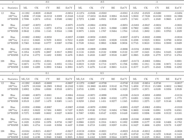
Table 6: Finite sample performance of alternative jackknife methods for the discrete time local to unit root model for m=2, where RE means the efficiency of CK relative to CY and the Exact CY (ExCY).

c -0.1 -0.5 -1

n Statistics ML CK CY RE ExCY ML CK CY RE ExCY ML CK CY RE ExCY 12 Bias -0.1282 -0.0628 -0.0649 -0.0654 -0.1274 -0.0586 -0.0582 -0.0581 -0.1252 -0.0523 -0.0490 -0.0494 100*Var 5.6936 17.8166 16.0152 0.8989 15.9443 5.8142 17.6853 16.0648 0.9084 16.0445 5.9833 17.7638 16.6100 0.9350 16.5966 10*RMSE 2.7086 4.2674 4.0541 0.9500 4.0462 2.7273 4.2460 4.0501 0.9538 4.0475 2.7481 4.2471 4.1049 0.9665 4.1037 36 Bias -0.0467 -0.0072 -0.0074 -0.0075 -0.0476 -0.0064 -0.0056 -0.0055 -0.0483 -0.0047 -0.0024 -0.0031 100*Var 0.7118 1.5215 1.3273 0.8724 1.3183 0.7486 1.5419 1.3815 0.8960 1.3809 0.7962 1.6061 1.5323 0.9541 1.5192 10*RMSE 0.9642 1.2356 1.1545 0.9344 1.1506 0.9875 1.2434 1.1767 0.9464 1.1764 1.0145 1.2682 1.2381 0.9763 1.2329 48 Bias -0.0362 -0.0062 -0.0058 -0.0057 -0.0369 -0.0050 -0.0035 -0.0037 -0.0374 -0.0032 -0.0006 -0.0016 100*Var 0.4111 0.8685 0.7670 0.8831 0.7652 0.4320 0.8887 0.8201 0.9228 0.8188 0.4598 0.9225 0.9031 0.9790 0.8850 10*RMSE 0.7365 0.9340 0.8777 0.9397 0.8766 0.7539 0.9441 0.9063 0.9600 0.9056 0.7745 0.9610 0.9504 0.9889 0.9409 96 Bias -0.0186 -0.0012 -0.0012 -0.0012 -0.0190 -0.0009 -0.0006 -0.0006 -0.0194 -0.0003 0.0004 0.0002 100*Var 0.1054 0.2276 0.2007 0.8817 0.2002 0.1116 0.2335 0.2122 0.9090 0.2122 0.1197 0.2421 0.2284 0.9435 0.2269 10*RMSE 0.3744 0.4772 0.4482 0.9391 0.4476 0.3845 0.4833 0.4607 0.9533 0.4607 0.3965 0.4920 0.4779 0.9713 0.4764 108 Bias -0.0166 -0.0014 -0.0014 -0.0014 -0.0170 -0.0010 -0.0006 -0.0007 -0.0173 -0.0003 0.0004 0.0001 100*Var 0.0871 0.1770 0.1585 0.8955 0.1584 0.0919 0.1828 0.1713 0.9375 0.1706 0.0981 0.1911 0.1886 0.9871 0.1842 10*RMSE 0.3388 0.4209 0.3983 0.9464 0.3983 0.3475 0.4276 0.4140 0.9681 0.4131 0.3577 0.4371 0.4343 0.9936 0.4292 c 0.1 0.5 1

n Statistics ML/LS CK CY RE ExCY ML/LS CK CY RE ExCY ML CK CY RE ExCY 12 Bias -0.1282 -0.0645 -0.0680 -0.0687 -0.1273 -0.0667 -0.0730 -0.0740 -0.1245 -0.0654 -0.0746 -0.0817 100*Var 5.6379 18.0168 16.2905 0.9042 16.2342 5.5331 18.3860 16.8083 0.9142 16.7762 5.4058 17.9513 15.5308 0.8652 14.9662 10*RMSE 2.6982 4.2934 4.0930 0.9533 4.0874 2.6745 4.3395 4.1643 0.9596 4.1623 2.6373 4.2871 4.0109 0.9356 3.9539 36 Bias -0.0460 -0.0073 -0.0081 -0.0084 -0.0444 -0.0071 -0.0090 -0.0100 -0.0418 -0.0059 -0.0093 -0.0124 100*Var 0.6940 1.5167 1.3112 0.8645 1.2961 0.6597 1.5183 1.3030 0.8582 1.2771 0.6201 1.5033 1.2518 0.8327 1.1778 10*RMSE 0.9519 1.2337 1.1479 0.9305 1.1415 0.9259 1.2343 1.1451 0.9277 1.1345 0.8913 1.2275 1.1227 0.9146 1.0923 48 Bias -0.0358 -0.0066 -0.0067 -0.0067 -0.0346 -0.0070 -0.0080 -0.0085 -0.0327 -0.0063 -0.0084 -0.0103 100*Var 0.4012 0.8622 0.7494 0.8691 0.7437 0.3825 0.8536 0.7242 0.8484 0.7066 0.3603 0.8436 0.6981 0.8276 0.6561 10*RMSE 0.7275 0.9309 0.8682 0.9327 0.8650 0.7087 0.9265 0.8547 0.9225 0.8449 0.6833 0.9206 0.8398 0.9122 0.8165 96 Bias -0.0184 -0.0013 -0.0015 -0.0015 -0.0177 -0.0012 -0.0018 -0.0020 -0.0166 -0.0009 -0.0021 -0.0029 100*Var 0.1025 0.2258 0.1976 0.8750 0.1967 0.0968 0.2225 0.1916 0.8615 0.1892 0.0899 0.2177 0.1830 0.8406 0.1762 10*RMSE 0.3691 0.4754 0.4448 0.9356 0.4437 0.3580 0.4718 0.4382 0.9287 0.4354 0.3427 0.4666 0.4283 0.9178 0.4207 108 Bias -0.0164 -0.0015 -0.0017 -0.0017 -0.0158 -0.0016 -0.0021 -0.0023 -0.0148 -0.0012 -0.0023 -0.0028 100*Var 0.0847 0.1753 0.1549 0.8837 0.1545 0.0801 0.1730 0.1508 0.8718 0.1495 0.0742 0.1700 0.1470 0.8648 0.1443 10*RMSE 0.3342 0.4190 0.3940 0.9403 0.3935 0.3243 0.4162 0.3889 0.9344 0.3873 0.3100 0.4125 0.3841 0.9311 0.3809

The data generating process considered is:

yt=βyt−1+t, εt∼ iidN(0,1), t= 1,2, . . . , n,

withβ= 1 +c/n, (−∞< c <∞),following Phillips (1987) and Chan and Wei (1988). We investigate the finite sample performance of alternative estimates ofβ using a sample size ranging from 12 to 108. The local to unity parametercis set to be 0.1, 0.5 and 1 for the local to unity from the explosive side, and−0.1,−0.5 and−1 for the local to unity from the stationary side.

Several interesting results emerge from these tables. Firstly, the bias in the estimate of β(orκ) is very similar for the CK method and the CY method in all cases. Secondly, the variance in the estimate ofβ(orκ) for the CY method is significantly smaller than that for the CK method in each case, the reduction in the variance being about 10% in all cases. Consequently, the RMSE is smaller for the CY method. Thirdly, although the exact CY method provides a smaller variance, the difference between the two CY methods is so small, suggesting that the proposed CY works well. Thus, it is not necessary to bear the additional computational cost associated with calculating the variances and covariances

from the finite sample distributions. Finally, whenm= 3, the variance of our CY estimator variance approximates more closely that of MLE, compared to that of CK. Although not reported here, this result is true for allm, including the optimalm used in CK.

4

Conclusion

This paper has introduced a new jackknife procedure for unit root models that offers an improve-ment over the jackknife methodology of CK (2013). The proposed estimator is optimal in the sense that it minimizes the variance of the jackknife estimator while removing the first order bias. The new method works well for the discrete time unit root model, the continuous time unit root model and the local to unit root model. Simulations have shown that the new method reduces the variance by about 10% relative to the estimator of CK without compromising the bias. The results hold true when an optimal number of subsamples is used. There exist some other models for which the asymptotic theory depends on the initial condition. Examples include explosive processes. It may be interesting to extend the results in the present paper to cover these models, although it is not pursued in the present paper. It is useful to point out that for a unit root model with an unknown intercept case, although fitting an intercept increases the bias of LS estimator, the asymptotic theory does not depend on the initial value.

5

Appendix

Proof of Lemma 2.1: Taking the derivative of MGF with respect toθ1, we get:

∂Ma,b,c,d(θ1,−θ2, ϕ1,−ϕ2)

∂θ1

=E[N(a, b) exp(θ1N(a, b)−θ2D(a, b) +ϕ1N(c, d)−ϕ2D(c, d))].

Settingθ1= 0, taking the derivative with respect to ϕ1, and then evaluating it atϕ1= 0, we have,

∂ _∂M a,b,c,d(θ1,−θ2, ϕ1,−ϕ2) ∂θ1 |θ1=0 /∂ϕ1 |ϕ1=0=E{N(a, b)N(c, d) exp [−θ2D(a, b)−ϕ2D(c, d)]}. Consequently, Z ∞ 0 Z ∞ 0 ∂ _∂M a,b,c,d(θ1,−θ2, ϕ1,−ϕ2) ∂θ1 |θ1=0 /∂ϕ1|ϕ1=0 dθ2dϕ2 = E N(a, b) D(a, b) N(c, d) D(c, d) .

Proof of Proposition 2.2: It can be found in Chen and Yu (2011).

References

Bao, Y., A. Ullah, and V. Zinde-Walsh, On Existence of Moment of Mean Reversion Estimator in Linear Diffusion Models. Economics Letters (2013), 120, 146-148.

Chambers, M.J., Jackknife estimation and inference in stationary autoregressive models. Journal of Econometrics (2013) 172, 142–157.

Chambers, M.J., and M. Kyriacou, Jackknife estimation with a unit root, Statistics & Probability Letters (2013), 83, 1677-1682.

Chan, N. H. and C.Z. Wei, Limiting distributions of least squares estimates of unstable autoregressive processes. Annals of Statistics (1988), 16, 367-401.

Chen, Y. and J. Yu, Optimal Jackknife for Discrete Time and Continuous Time Unit Root Models, Singapore Management University, Working Paper, 12-2011, (2011).

Efron, B, Bootstrap methods: another look at the jackknife. The Annals of Statistics (1979), 1-26.

Magnus, J.R., The exact moments of a ratio of quadratic forms in normal variables. Aunales d’Economie et de Statistique (1986) 4, 95-109.

Hall, P. The bootstrap and Edgeworth expansion (1992), New York: Springer-Verlag.

Kendall, M. G., Note on bias in the estimation of autocorrelation. Biometrika (1954), 41(3-4), 403-404.

Phillips, P.C.B., Toward a unified asymptotic theory for autoregression,Biometrika (1987), 74, 533-547.

Quenouille, M. H., Approximate Tests of Correlation in Time-Series, Journal of the Royal Statistical Society (1949). Series B,11, 68-84.

Sargan, J. D., Econometric Estimators and the Edgeworth Approximation,Econometrica (1976), 44, 421–448.

Shao, J., and Tu, D. The Jackknife and Bootstrap (1995), Springer, New York.

White, J. S., Asymptotic Expansions for the Mean and Variance of the Serial Correlation Coefficient, Biometrika (1961), 48, 85-94.

Yu, J., Bias in the Estimation of the Mean Reversion Parameter in Continuous Time Models,Journal of Econometrics (2012), 169, 114-122.