Profit Maximization with Data Management Systems

ICIS 2005 Proceedings

International Conference on Information Systems

(ICIS)

12-31-2005

Profit Maximization with Data Management

Systems

Adir Even

Boston University School of Management

Ganesan Shankaranarayanan

Boston University School of Management

Paul Berger

Boston University School of Management

Follow this and additional works at:

http://aisel.aisnet.org/icis2005

This material is brought to you by the International Conference on Information Systems (ICIS) at AIS Electronic Library (AISeL). It has been accepted for inclusion in ICIS 2005 Proceedings by an authorized administrator of AIS Electronic Library (AISeL). For more information, please contact

[email protected].

Recommended Citation

Even, Adir; Shankaranarayanan, Ganesan; and Berger, Paul, "Profit Maximization with Data Management Systems" (2005).ICIS 2005 Proceedings.Paper 4.

M

S

Adir Even, G. Shankaranarayanan, and Paul D. Berger

Boston University School of Management

Boston, MA U.S.A.

[email protected]

[email protected]

[email protected]

Abstract

Data, a core component of information systems, has long been recognized as a critical resource to firms. Data is the backbone of business processes; it enables efficient operations, supports managerial decision-making, and generates revenues as a commodity. This study identifies a significant gap between the technical and the business perspectives of data management. While functionality and technical efficiency are well addressed, the consideration of economic perspectives, such as value-contribution and profitability, is not evident. This study suggests that introducing economic perspectives can better inform the design and the administration of data management systems by accounting for the interplay between business benefits and implementation costs. To address the identified gap, the paper proposes a quantitative microeconomic framework for data management that links value and cost to the impartial/technological characteristics of data and the related information system. Such a mapping allows cost/benefit assessment and determination of optimal configuration of system and data characteristics to maximize value and profits. The framework is demonstrated through development of a model for tabular datasets, and the optimal design of dataset characteristics (such as time-span, desired quality-level, and the set of attributes to be included). The application of the model is illustrated using numerical examples.

Keywords: Data management, information value, information economy, database, design, data quality, microeconomic modeling, utility, information product design

Introduction

Data has been recognized as a critical resource, essential at all business levels from day-to-day operations to strategic decision-making (Redman 1996). The amount of data managed by organizations is increasing; data warehouses in the magnitude of peta (1015_{) bytes have been recently reported. Data management efforts are directed toward the design and management of data}

activities (such as acquisition, processing, storage, and delivery), and corporate investments in data management technologies and services are steadily growing (Wixom and Watson 2001). Current data management activities and design methodologies are geared toward functionality and technical efficiency but, as the investments in these grow, concerns about the economic benefits of data assets also increase. For information-intensive firms (e.g., Reuters, AC-Nielsen, and S&P), the value gained from data products is the critical success factor, and data in such firms is perceived as a strategic asset (Glazer 1993). There is no significant research evidence for understanding the corporate gains from investments in data repositories and the related management activities. There is an emerging need to examine how such assets ought to be managed from the business-benefit viewpoint. This study brings together the economic and technical perspectives in information systems/information technology (IS/IT) management in general. Specifically, it examines data management, an IS/IT field in which the gap between the two perspectives is apparent. This study contributes to a better understanding of the business value and the profitability of data, the impact of economic factors on data management activities, and their implications for design and administration. The remainder of this paper is organized as follows. The next section provides the relevant background. The subsequent section proposes a microeconomic framework

for modeling the effect of data and system characteristics on both value and cost. This framework allows assessment of profitability, which can be maximized through an optimal design configuration. The framework in its general form targets a broad-range of system components and configuration factors. In this study, however, it is applied to the development of a quantitative model for the tabular dataset, the most common data-storage structure in data management systems. We then demonstrate the use of the model for profit maximization by configuring key tabular dataset characteristics: the time span, the data quality level, and the field structure, essentially addressing the design of tabular datasets in data repositories. Finally, concluding remarks are offered and directions for future research proposed.

Relevant Background

This section reviews relevant data management aspects and introduces research concepts that can influence a more rigorous economic thinking in this field. Data management has been the subject of substantial academic research and practitioner discussions. It is considered a complex task: data is integrated from multiple sources, processed and stored in repositories, and delivered by front-end tools or via exchange protocols. The collection of processes and systems forms a complex multistage architecture that can be viewed as a data manufacturing process (DMP). The output of the DMP is an information product (IP), a commodity that can be used internally, sold to other firms, or embedded within product offerings. The DMP/IP management is assisted by metadata, an abstraction of design and administration choices that represents different aspects of functionality and characteristics, such as infrastructure, model, process, contents, representation, and administration (Shankaranarayanan and Even 2004). The DMP/IP view is predominant in today’s data quality management (DQM) field, underlying the adaptation of total quality management principles (Wang 1998), and the development of quality improvement methodologies (Ballou et al. 1998; Redman 1996; Shankaranarayanan et al. 2003). The value gained by DQM is often discussed qualitatively (Redman 1996; Wang 1998), with the exception of the quantitative DMP optimization discussed by Ballou et al. (1998). Their model maps quality attributes to value and cost, an approach that underlies optimization models for quality trade-offs (Ballou and Pazer 1995, 2003), and influences the framework developed in this paper. Another key data management principle that influences this study is the separation of data and program. Datasets are held in independent database management systems (DBMS) that can be accessed by multiple applications. Leading data management technologies (e.g., RDBMS, flat-files, spreadsheets, and statistical packages) use a tabular-dataset model, based on two-dimensional structures that abstract business entities, and/or the relationships among them. This research focuses on key tabular-dataset characteristics that are further discussed in the next section.

While the technical aspects of data management are well-addressed, discussion of its economic aspects is surprisingly rare although information value (IV) and economics have attracted significant research attention within the broader context of IS/IT (Banker and Kauffman 2004), and have been an important focal point for field practitioners (Wixom and Watson 2001). A few key concepts have emerged from this stream. While firms are viewed as profit-maximizing entities, the profit contribution of IS/IT is often not apparent and difficult to prove empirically (Davern and Kauffman 2000). Organizations gain economic benefits from IS/IT through strategic alignment with business goals (Henderson and Venkatraman 1993). IS/IT value is shown to materialize through contextual use (Devaraj and Kohli 2003) and successful integration into business processes, together with complementary resources (Davern and Kauffman 2000). IV is often viewed as the payoff margin between perfect information versus imperfections that result in inferior outcome and lower willingness-to-pay (Banker and Kauffman 2004). IV is argued to be asymmetric: shared information may have different value to different actors (Lee et al. 2000; Raju and Roy 2000). Among the IV determinants (IS characteristics, managerial actions, payoffs, and uncertainties), only the IS characteristics (particularly quality) are shown to have monotonic relationships with value (Hilton 1981). Conversely, volume does not; increasing it might have negative effects when interactions among utilities (Arya et al. 1997) or uncertainties (Sulganik and Zilcha 1996) exist. Concepts of information value and economics can inform better data management from the business viewpoint. First, while data management focuses on technical and functional aspects, there is a need to measure performance within business context and choose the dependent variable (DV) accordingly (e.g., profitability). Profit maximization implies both value increase and cost reduction. While data management costs are reasonably well understood, the value gained is largely unknown and needs further study. Second, data is attributed with value only within contextual use, hence the need to link valuation of data with business usage. Third, although driven by use, value is influenced by impartial IS characteristics. IV models often treat information abstractly, rather than address specific technological characteristics. The utility function approach aims to address this challenge. Such functions map IS attributes into tangible value within specific usage, and attempt to maximize value through optimal design (Ahituv 1981). Utility functions are not commonly used in data management, although they are shown to be significant for DQM and DMP optimization (Ballou and Pazer 1995, 2003; Ballou et al. 1998). Microeconomic frameworks for value-driven data mining have embedded utility functions to help direct data search that yields patterns with the potential to generate concrete and

1

Alternative data models (e.g., object-oriented, object-relational, and XML) are gaining popularity in IS implementation and future extensions to this study should look into extending the framework to address those.

Contextual Usage

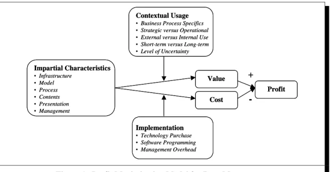
• Business Process Specifics • Strategic versus Operational • External versus Internal Use • Short-term versus Long-term • Level of Uncertainty Impartial Characteristics • Infrastructure • Model • Process • Contents • Presentation • Management Implementation • Technology Purchase • Software Programming • Management Overhead Value Cost Profit

+

-Contextual Usage

• Business Process Specifics • Strategic versus Operational • External versus Internal Use • Short-term versus Long-term • Level of Uncertainty Impartial Characteristics • Infrastructure • Model • Process • Contents • Presentation • Management Implementation • Technology Purchase • Software Programming • Management Overhead Value Cost Profit

+

-Figure 1. Profit Maximization Model for Data Management

profitable action (Kleinberg et al. 1998). These concepts—profitability as the DV, contextual value attribution, and the mapping of impartial/technological IS/IT characteristics to value and cost—guide the development of the microeconomic framework described next.

A Profit-Maximization Framework for the DMP/IP

The quantitative microeconomic framework, which stems from the DMP/IP view, assumes maximizing profit—the difference between the value gained by using IPs (the DMP output) and the cost of implementing the DMP—as the key goal of data management. It is assumed that both value and cost are affected by impartial characteristics of the DMP and/or the IP that are captured in the metadata abstraction. The effect of these characteristics on value is assumed to be moderated by contextual usages and their effect on cost by implementation factors (Figure 1). The model highlights three paths to increase profit: (1) increasing IP usage, (2) reducing DMP implementation costs, and (3) optimizing DMP/IP configuration. This microeconomic model coincides with the view of design as a process of searching for optimality among feasible solutions (Churchman 1971). This study posits that models, such as the one described here, promote value-driven and profit-maximizing design and, hence, contribute to better data management. Value and profit optimization models are common in marketing and operations management research, particularly in the field of product design. Such models underlie the optimal design and configuration of products (e.g., Kohli and Sukumar 1990) and services (e.g., Easton and Pullman 2001; Eriksen and Berger 1987). They are also used for cost-benefit optimization of production lines (e.g., Cooper and Slagmulder 2004; Yigit et al. 2002).

To develop the model, this paper first describes the general formulation of the key constructs by taking a deterministic approach. This is then extended for tabular datasets.1

Metadata Vector (X): The metadata vector X represents the set of input characteristics that are subject to optimal configuration. Metadata characteristics can be broadly classified as design or maintenance, a categorization that reflects different optimization options at different stages of the system implementation cycle. Design characteristics reflect the long-term decisions that are typical in early stages (e.g., infrastructural and architectural choices), while maintenance characteristics reflect the short-term, ongoing decisions that are made when the system is operational (e.g., performance monitoring and troubleshooting). Data management systems introduce a large set of configuration decisions. To minimize complexity, it is important to limit the input

2

Such assumptions reflect a primarily internally (within an organization) focused usage. With external use, increasing volumes and improving quality above certain levels can create new usage opportunities and the resulting demand curves are more likely to follow an S-shape. These are to be explored in future extensions.

set to include only those characteristics that significantly affect value and/or cost and, hence, profitability. In the specific case of the tabular dataset, the following key design characteristics significantly affect the value and the cost.

Field Structure ({Ym}m=1..M): In the tabular dataset model, entity attributes are represented by fields or columns. Attributes are

not necessarily of equal importance from the business perspective. An optimal field-structure design has to consider trade-offs: a small set forms a parsimonious abstraction of the entity, simplifies data acquisition and processing, decreases size, and results in lower storage and administration costs. An over-simplified set, on the other hand, might fail to capture important descriptors, and thus prevent the integration of the dataset within business processes and reduce the potential for gaining value. While some fields may be mandatory for all possible uses, or needed for maintenance purposes (e.g., time indicators or index fields), others may be optional and their inclusion or exclusion is subject to design decisions. We assume M optional fields, each represented by a variable Y_m, a binary integer: Y_m = 1 implies a decision to include the field [m] in the dataset, while Y_m = 0 implies exclusion.

Time Span (T): Entity instances in a tabular dataset are represented as records, or rows, with identical field structure. The number of records (N) introduces profitability trade-offs: a larger N often implies higher costs (e.g., upgrades to storage space, hardware, and applications). On the other hand, a larger N offers a broader and more granular business perspective and allows more elaborate analysis. To address this trade-off, databases are often segmented by record age: the more recent data is made available to end-users via an active dataset, optimized for fast performance, while older data is discarded or archived. The time span covered by the active dataset, determined by an age cut-off, dictates the expected N and hence becomes an important design factor. The time span is represented as a nonnegative, continuous variable, T = 0. N is assumed to be linear with T: N(T) = RT where

R is the record density per time period.

Quality Level (Q): Data quality (DQ) is commonly evaluated along a set of attributes (e.g., accuracy and completeness), and measured as a ratio within the range of 0 (bad) and 1 (good) (Pipino et al. 2002). DQ can be measured impartially, based on the dataset structure and/or contents (e.g., reflecting undamaged data), or contextually, within a specific business usage (e.g., reflecting task-relevant data). DQM literature has discussed a plethora of DQ solutions, from error detection and correction, to comprehensive process design methodologies (Redman 1996; Wang 1998). In the proposed model, the quality level is viewed as a design target (conversely, in other decision scenarios, it can be viewed as reflecting the actual status). Designing the system that guarantees the high quality of the generated dataset(s) increases the potential to gain value, but might imply investments in costly DQ solutions. The model proposed here optimizes the targeted level of one DQ attribute, measured impartially. A dataset record is assumed to be either of good quality with likelihood Qr or of poor quality with likelihood of (1-Qr). The overall dataset quality Q is a number between 0 and 1, defined as the proportion of good-quality records. It can be shown that Q = Qr, assuming that record quality levels are independent and identically distributed variables.

Value: Data (or IP) value is attributed within contextual business use and reflects the consumer’s willingness-to-pay, hence is measured monetarily. Impartial DMP/IP characteristics can affect the value, some directly (e.g., dataset richness, promptness of delivery, or accuracy), and others indirectly (e.g., hardware and process configurations). The characteristic-to-value mapping is represented as a set of utility functions, one per usage scenario. The contextual moderation effect is reflected in the specific functional form. The overall value is sum-additive:

(1)

( )

X

=

∑

i= I

U

i

( )

X

U

.. 1

where X = The metadata vector of impartial characteristics

Ui = Utility within contextual usages, indexed by [i]

I = The total number of contextual usages

U = The overall value

A tabular dataset can serve multiple purposes. Considering time (T) and quality (Q) first, the value within a use scenario is assumed to be capped and maximized with the longest possible time range (T Æ4) and optimal quality (Q = 1). The value degrades with lower quality level and is assumed to have an exponentially diminishing return with age.2 _{It is hence represented}

(2)

(

_T

_Q

)

_k

(

_e

i

)

_Q

i

U

_i

,

=

_i

1

−

−αT β where U_i (T, Q)= The value of usage scenario [i]

ki = The value cap of usage scenario [i], at Q=1 and TÆ4

"i = A positive exponential slope factor of usage scenario [i]. The greater the value of "i, the less dependent the usage scenario is on older data.

$i = A positive quality sensitivity factor of usage scenario [i]. The greater the value of $i, the more sensitive the user scenario is to loss of quality.

The overall value for all use scenarios is therefore given by

(3)

(

_T

_Q

)

_k

(

_e

i

)

_Q

i

U

I i T i β α

∑

= −

−

=

_1..

1

,

Adding structure characteristics (X = [T, Q, {Y_m}]), each use scenario may require a different field subset. Some fields are mandatory for a certain scenario, some are not mandatory but may reduce value if excluded, and yet others do not affect the scenario at all. We define

0i

m _{as the sensitivity factor of usage [i] to optional field [m], 0 < 0}

i

m _{< 1. The higher the 0} i

m_{, the more necessary the field. 0} i m

= 1 implies a mandatory field for usage [i]. 0i

m _{= 0 implies that usage scenario [i] is independent of the inclusion of field [m].}

is the effect of field [m] on usage scenario [i]. With sensitivity factor 0_im _{= 0, the effect is always 1. With}

(

m

)

m i m i

Y

s

=

1

−

η

1

−

sensitivity factor 0i

m _{= 1, the effect is 1 if the field is included and 0 if not. With 0 < 0} i

m _{< 1, the effect is 1 if the field is included,} and 1 - 0i

m _{if not.}

is the structure effect on usage [i]. Excluding a mandatory field implies Si = 0.

(

)

(

)

∏

∏

=

=

=

−

−

=

_{m M} m m i M m m i i

s

Y

S

_{1.. 1..}

1

η

1

Excluding a partially important field (0 < 0 < 1) reduces Si but not to 0. Fields of which the scenario is independent do not affect the overall value (since si

m _{= 1).}

Adding field structure considerations to (3), the overall value is given by

(4)

{ }

(

)

_∑

(

)

_∑

₌

(

−

)

[

_∏

₌

(

(

)

)

]

= −

₌

₋

₋

₋

−

=

_{m M} m m i I i T i i I i T i

e

Q

S

k

e

Q

Y

k

Y

Q

T

U

i i i i .. 1 .. 1 .. 1

1

1

1

1

,

,

α β α β

η

ki is now interpreted as the maximum potential value of scenario [i], given full time span covered (T Æ4), optimal quality level (Q = 1) and all the value-contributing fields included.

Cost: The DMP implementation comes at a cost, which is driven by technical and managerial decisions such as infrastructural choices, programming efforts, investment in quality improvement solutions, and administrative overhead. Similar to utility, DMP characteristics affect the cost directly or indirectly. Cost factors can be represented as a parameterized function that translates the effect of impartial characteristic to monetary output.

(5)

( )

X

=

∑

j= J

C

j

( )

X

C

_1..

where X = The metadata vector of impartial characteristics

Cj = Cost factor, indexed by [j]

J = The total number of cost factors

C = The overall cost

(6)

(

T

Q

)

C

C

( )

T

C

(

T

Q

)

C

,

=

_f

+

_l

+

_q

,

where C_f = A fixed component, which can be related, for example, to hardware or networking.

Cl (T) = A linear component with a per-record cost cl, which can be related to data acquisition or to investment in disk-storage space. The linear cost is, hence, given by

(7)

( )

T

c

N

( )

T

c

RT

C

_l

=

_l

=

_l

C_q(T,Q) = Variable quality cost. Often, the older the data is, the more expensive it is to maintain its quality. The quality cost per record is therefore assumed to be

(8)

( )

t

Q

c

Q

(

t

)

c

Q

(

t

)

C

_qR

,

=

_{q r}δ

1

+

θ

=

_q δ

1

+

θ

where t = The age of the record.

Qr (=Q) = Quality level of a single record.

c_q = Cost of maintaining a record of age 0 at a maximum quality level.

* = Cost sensitivity to the quality, * > 1. The greater * is, the greater is the increase in cost as perfect quality is approached.

2 = Cost sensitivity to age, assuming linear increase. 2 > 0, where equality to zero reflects no age effect on quality cost per record.

The record density is R. Therefore, the overall quality cost and the overall cost are

(9)

(

)

( )

(

)

(

2

)

.. 0 .. 0

,

1

0

.

5

,

Q

RC

Q

d

c

RQ

d

c

RQ

T

T

T

C

_q T q T R q q

τ

τ

θτ

τ

θ

δ τ δ τ

=

+

=

+

=

∫

₌

∫

₌ (10)

(

)

( )

(

)

(

2

)

5

.

0

,

,

Q

C

C

T

C

T

Q

c

c

RT

c

RQ

T

T

T

C

=

_f

+

_l

+

_q

=

_f

+

_l

+

_q δ

+

θ

Adding field structure characteristics may affect each cost component.

Fixed cost (C_f): The fixed cost is assumed to have a fixed component c_f0_{. Each optional field, if included, adds an incremental} cost cf

m _{(e.g., design and programming efforts related to adding the field). The fixed cost is hence given by}

(11)

{ }

( )

_{m M} m m f f f

Y

c

c

Y

c

*

.. 1 0

∑

=

+

=

Linear Cost (Cl): The per-record cost cl, is assumed to have a fixed component cl

0_{, (potentially attributed to mandatory fields).} Each optional field, if included, adds an incremental cost c_lm_{. The linear cost, as derived from (7), is hence given by}

(12)

{ }

(

T

Y

)

(

c

c

Y

)

RT

C

_m M m m l l l

,

_1..

*

0

∑

=

+

=

Quality Cost (Cq): Similarly, the per-record quality cost cq, is assumed to have a fixed component cq

0_{, and each optional field,} if included, adds an incremental quality cost per record cq

m_{. The quality cost, as derived from (10), is, hence, given by}

(13)

{ }

(

)

(

)

(

2

)

.. 1 0

5

.

0

*

,

,

Q

Y

c

c

Y

RQ

T

T

T

C

_{m M} m m q q q

θ

δ

₊

+

=

∑

₌

(14)

{ }

(

)

(

) (

)

(

)

(

2

)

.. 1 0 .. 1 0 .. 1 0

5

.

0

*

*

*

,

,

T

T

RQ

Y

c

c

RT

Y

c

c

Y

c

c

Y

Q

T

C

m M m m q q m M m m l l m M m m f f

θ

δ

₊

+

+

+

+

+

=

∑

=

∑

∑

= =

Profit: The profit is defined as the difference between overall value and overall cost.

(15)

( )

X

=

U

( ) ( )

X

−

C

X

=

∑

i= I

U

i

( )

X

−

∑

j= J

C

j

( )

X

P

_{1.. 1..}

where X = A vector of metadata characteristics.

{Ui(X)} = Value attributed to I contextual usages, indexed by [i].

{Cj(X)} = Cost attributed to J cost factors, indexed by [j].

P(X) = Contribution of data to profit.

P(X) is the objective function for the optimization problem: configure the characteristics of the DMP/IP (the vector X) such that the overall profit is maximized. Optimal configuration is subject to constraints such as target business goals, legal and contractual obligations, capped implementation budget and time, scarcity of required resources, or interdependency among metadata components. With tabular datasets, considering T and Q first, profit is given by

(16)

(

)

(

)

(

(

2

)

)

.. 1

1

0

.

5

,

Q

k

e

Q

c

c

RT

c

RQ

T

T

T

P

_{f l q} I i T i i i β δ

θ

α

₋

₊

₊

₊

−

=

∑

₌ − s.t. T > 0, Q > 0, Q < 1

Adding field structure characteristics yields

(17)

{ }

(

)

(

)

[

(

(

)

)

]

(

) (

) (

)

(

)

[

2

]

.. 1 0 .. 1 0 .. 1 0 .. 1 .. 1

5

.

0

*

*

*

1

1

1

,

,

T

T

RQ

Y

c

c

RT

Y

c

c

Y

c

c

Y

Q

e

k

Y

Q

T

P

m M m m q q m M m m l l m M m m f f M m m m i I i T i i i

θ

η

δ β α

+

+

+

+

+

+

−

−

−

−

=

∑

∑

∑

∏

∑

= = = = = −

s.t. T > 0, Q > 0, Q < 1,Y_m > 0, Y_m < 1 and Y_m integer, for each m = 1…M

While the profitability has apparent trade-offs with T, Q, and {Ym}, the effect of other parameters can be inferred from the profit model. We expect profitability to

• Increase with I and {k_i}: more usages and higher per-use value increase profitability.

• Increase with " and decrease with $: higher time sensitivity implies near optimality with less time coverage, higher quality sensitivity implies higher decline as quality degrades.

• Decrease with 0i

m_{: profitability is likely to reduce with higher sensitivity to field exclusion.} • Decrease with c_f, c_l, and c_q: higher cost factors decrease profitability.

• Decrease with * and 2: higher quality cost sensitivity to Q or to T decreases profitability.

Future Extensions: Data management systems are complex and in reality profitability can be affected by a large set of other characteristics (e.g., infrastructure, process, and delivery). The usability of such a framework depends on identifying a limited subset of influential characteristics and modeling their effect on value and cost. The general formulation assumes determinism for simplicity, although in reality data management systems are far from being deterministic. Alternative formulations can consider stochastic behavior and transform the optimization problem (15) into maximization of expectation over time (denoted

Et[]). (18)

( )

X

=

E

t

[

U

( )

X

]

−

E

t

[

C

( )

X

]

=

∑

i= I

E

t

[

U

i

( )

X

]

−

∑

j= J

E

t

[

C

j

( )

X

]

P

.. 1 .. 1

Another underlying assumption to be reconsidered is the sum-additive modeling of utility and cost factors. This assumption, while simplifying the model analytically, suggests that such factors are independent of each other, which often does not reflect real-life

3

Microsoft-Excel/Solver was used for the numeric illustrations in this study.

practices. Value enhancement or neutralizing relationships may exist among utilities and costs, in which case the whole is not necessarily an additive-sum of the parts. Such scenarios of interdependency ought to be further explored, and the framework should be enhanced to model them properly.

Other model enhancements to consider are, for example

• Different constraints on T and Q (Tmin _{< T < T}max_{, Q}min _{< Q < Q}max_{), dictated by business needs.} • Uneven distribution of records along time, which implies a different N(T) formulation.

• Quality levels per record that are not i.i.d., which implies a different Q formulation.

• Different functional forms (e.g., step or s-shaped) for mapping T, Q, and {Ym} to cost and value: information overload, for example, might imply value degradation as volume and field structure complexity increase. Larger T and Q, and/or richer field structure may introduce new usage opportunities, but require significant hardware and software upgrade.

Optimal Configuration of Tabular-Dataset Characteristics

This section demonstrates the use of the profit-maximization framework for optimal design of dataset characteristics. The optimization model is nonlinear and mixes continuous and integer input variables. Still, within certain assumptions, a closed-form solution can be obtained. More often, however, optimization requires numerical approximation, using dedicated software.3

Optimizing the Time Span (T) and the Quality Level (Q)

With certain relaxations, closed-form solutions can be obtained for optimizing T and Q. Three cases are demonstrated: (1) optimizing T alone, (2) optimizing Q alone, and (3) optimizing T and Q simultaneously.

Case 1: Optimizing the time span alone, given Q. A first derivative of (16) yields

(19)

(

T

Q

)

T

k

e

Q

c

R

c

RQ

c

RQ

T

P

_{l q q} I i T i i i i

θ

α

α β

₋

₋

δ

₋

δ

=

∂

∂

∑

₌ − .. 1

/

,

The optimal time span can be obtained from MP(T,Q)/MT=0, or

(20)

T

RQ

c

RQ

c

R

c

Q

e

k

_{l q q} I i T i i i i

θ

α

α β

₌

₊

δ

₊

δ

∑

= − .. 1

Since the left-hand side is monotonically decreasing with T and the right-hand side is monotonically increasing with T, there is a single TOPT _{solution. Taking a second derivative}

(21)

θ

α

α β δ

RQ

c

Q

e

k

T

P

_{i I} q T i i i i

−

−

=

∂

∂

∑

₌ − .. 1 2 2 2

/

The second derivative is negative. Hence, TOPT _{is a point of maximal profitability. A closed-form solution can be obtained from}

(20) for a single utility (I = 1) and assuming 2 = 0.

(22)

δ β

α

α

ke

− T

Q

=

c

_l

R

+

c

_q

RQ

This optimum represents the time point above which the marginal cost (

c

_l

R

+

c

_q

RQ

δ) exceeds the marginal value (

α

ke

−αT

Q

β). The optimal time can now be obtained from (22).

(23)

(

)

⎪⎩

⎪

⎨

⎧

⎪⎭

⎪

⎬

⎫

+

=

_−β

α

_δ

α

RQ

c

c

Q

k

Ln

T

q l OPT

1

The maximum profitability is given by

(24)

(

)

(

)

f q l q l OPT

c

Q

c

c

RQ

k

e

Ln

Q

c

c

R

kQ

Q

T

P

−

⎪⎭

⎪

⎬

⎫

⎪⎩

⎪

⎨

⎧

+

+

−

=

₋

)

(

*

*

,

β δ _β

α

_δ

α

Case 2: Optimizing Q alone, given T. A first derivative of (16) yields

(25)

(

)

(

)

1 1

(

2

)

.. 1

1

0

.

5

/

,

Q

Q

k

e

Q

c

RQ

T

T

T

P

_{i I} q T i i i i

δ

θ

β

₋

α β

₋

δ

₊

=

∂

∂

− − = −

∑

The optimal quality level be obtained from MP(T,Q)/ MQ = 0, or

(26)

(

)

1 1

(

2

)

.. 1 I

k

1

e

Q

c

q

RQ

T

0

.

5

T

i T i i i i

δ

θ

β

₋

α β −

₌

δ−

₊

= −

∑

Such equation may have more than one solution, depending on the actual parameter values. A solution below 0 implies that the system is infeasible; when a solution is above 1, the constraint Q < 1 applies, and Q = 1 is the candidate choice. The second derivative yields (27)

(

)

(

)

(

)

(

)

2

(

2

)

.. 1 2 2 2

5

.

0

1

1

1

/

,

Q

Q

k

e

Q

c

RQ

T

T

T

P

_q I i T i i i i i

δ

δ

θ

β

β

₋

₋

α β

₋

₋

δ

₊

=

∂

∂

− = − −

∑

With * > 1, the second derivative is negative if 0 <$i < 1 and the optimal solution, if feasible (0 < Q < 1), indicates maximal profitability. If $i > 1, the second derivative is not guaranteed to be negative. Hence, there is a need to obtain its value with the actual parameters. A closed-form solution can be obtained from (26) for a single utility (I = 1):

(28)

(

)

1 1

(

2

)

5

.

0

1

e

Q

c

RQ

T

T

k

T

δ

_q

θ

β

₋

−α β−

₌

δ−

₊

This optimum represents marginal cost

(

δ

c

q

RQ

1

(

T

0

.

5

θ

T

2

)

)

exceeding the marginal value . The

δ−

₊

(

(

)

1

)

1

−

−α β−

β

k

e

T

Q

optimum can be now obtained from (28):

(29)

(

)

(

)

β δ α

θ

δ

β

− −

⎟

⎟

⎠

⎞

⎜

⎜

⎝

⎛

+

−

=

1 2

5

.

0

1

T

T

R

c

e

k

Q

q T OPT

If 0 < QOPT _{< 1, the maximal profitability is given by}

(30)

(

)

(

)

(

(

2

)

)

5

.

0

1

,

Q

k

e

Q

c

c

RT

c

RQ

T

T

T

P

=

−

−αT OPTβ

−

_f

+

_l

+

_q OPTδ

+

θ

Otherwise, QOPT _{< 0 implies unfeasibility and if Q}OPT _{> 1, Q}OPT _{= 1 is optimal and profitability is}

(31)

( )

(

)

(

)

2

5

.

0

1

1

,

k

e

c

c

c

RT

c

RT

T

P

=

−

−αT

−

_f

−

_l

+

_q

−

θ

_q

Case 3: First derivatives by T and by Q are given by (19) and (25) respectively. Solving MP/MT = 0 and MP/MQ = 0 simultaneously yields candidate solutions, which can be checked for optimality. With the simplifying assumptions of I = 1, c_l = 0 and 2 = 0, and (32)

(

_T

_Q

)

_T

_α

_ke

α

_Q

β

_c

_RQ

δ

P

q T

₋

=

∂

∂

_,

_/

−

_P

(

_T

_Q

)

_Q

_k

(

_e

)

_Q

_c

_RQ

_T

q T 1 1

1

/

,

∂

=

−

− −

−

−

∂

_β

α β

_δ

δ Solving MP/MT = 0 and MP/MQ = 0 and (33) δ β α

α

ke

− T

Q

=

C

_q

RQ

β

k

(

1

−

e

−αT

)

Q

β

=

δ

C

_q

RQ

δ

T

Dividing the second equation by the first yields

(34)

(

T

)

OPT

T

e

OPT

δ

α

β

α

−

1

=

Since * > 0, the equation has a positive TOPT _{solution (in addition to T = 0). Substituting *T in the second equation yields a} candidate QOPT_{, which should be checked for feasibility (0 < Q < 1).}

(35)

(

)

(

α

)

δ β α

α

− −

⎟⎟

⎠

⎞

⎜⎜

⎝

⎛

−

−

=

1 0

1

1

T T OPT

e

R

C

e

k

Q

For checking optimality, the Hessian matrix and its determinant should be looked at.

(36)

(

)

[

]

(

)

(

)

(

)

(

)

(

)

⎥

⎥

_⎦

⎤

⎢

⎢

⎣

⎡

−

−

−

−

−

−

−

−

−

−

−

=

⎥

⎦

⎤

⎢

⎣

⎡

∂

∂

∂

∂

∂

∂

∂

∂

∂

∂

=

− − − − − − − − − −

T

RQ

c

Q

e

k

RQ

c

Q

e

k

RQ

c

Q

e

k

Q

ke

Q

P

T

Q

P

Q

T

P

T

P

Q

T

P

H

q T q T q T T 2 2 1 1 1 1 2 2 2 2 2 2 2

1

1

1

1

1

/

/

/

/

,

δ β α δ β α δ β α β α

δ

δ

β

β

δ

αβ

δ

αβ

α

(37)

(

₂

)

2 2 2 2 2

/

/

*

/

T

P

Q

P

T

Q

P

D

=

∂

∂

∂

∂

−

∂

∂

∂

The following conditions can be evaluated to determine optimality:

• If D > 0 and second derivatives are positive at (TOPT_{, Q}OPT_{), the point is a relative minimum.} • If D > 0 and second derivatives are negative at (TOPT_{, Q}OPT_{), the point is a relative maximum.} • If D < 0, the point is a saddle point and if D = 0, higher order tests must be used.

Illustrative Example 1: A firm wishes to promote a product to listed customers. Targeting the entire list is expected to yield $1 million. The list covers 25 years with an average of 10,000 customers added per year. The more recent a customer, the higher is the acceptance chance, with a marginal exponential decline rate of 0.2. Often, customer information is inaccurate and damages promotion efforts with a sensitivity rate of 2. Raising quality level to 100 percent accuracy is viable, but expensive ($6 per record), with negligible increase for older data. However, a cheaper mix of automated and manual procedures can lower cost, with a quality cost sensitivity factor of 5. Since the list is already in place, fixed costs and per-record marginal cost are negligible. To optimize the expected profit, two questions must be addressed: (1) how many years of customer data should be included, and (2) what data quality level should be targeted?

Translation of the given problem to the model parameters yields

Time Span Optimization -1,000,000 -500,000 0 500,000 1,000,000 1,500,000 2,000,000 0 2 4 6 8 10 12 14 16 18 20 22 24 Time Span (T) $ A m ou nt Value Cost Profit

Time Span Optimization

-1,000,000 -500,000 0 500,000 1,000,000 1,500,000 2,000,000 0 2 4 6 8 10 12 14 16 18 20 22 24 Time Span (T) $ A m ou nt Value Cost Profit

Quality Level Optimization

-1,000,000 -500,000 0 500,000 1,000,000 1,500,000 2,000,000 0.00 0.10 0.20 0.30 0.40 0.50 0.60 0.70 0.80 0.90 1.00 Quality Level (Q) $ A m ount Value Cost Profit

Quality Level Optimization

-1,000,000 -500,000 0 500,000 1,000,000 1,500,000 2,000,000 0.00 0.10 0.20 0.30 0.40 0.50 0.60 0.70 0.80 0.90 1.00 Quality Level (Q) $ A m ount Value Cost Profit

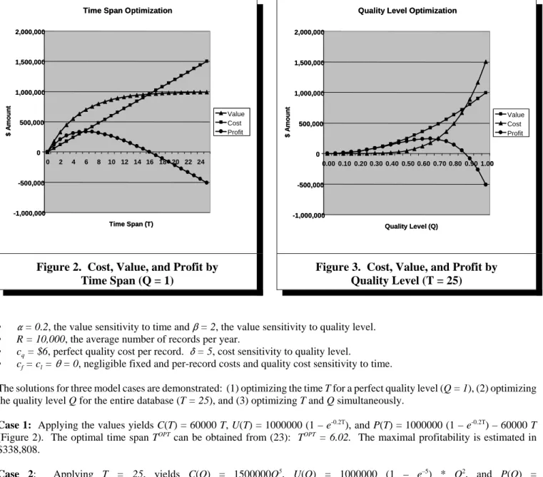
Figure 2. Cost, Value, and Profit by

Time Span (Q = 1)

Figure 3. Cost, Value, and Profit by

Quality Level (T = 25)

• " = 0.2, the value sensitivity to time and $ = 2, the value sensitivity to quality level. • R = 10,000, the average number of records per year.

• cq = $6, perfect quality cost per record. * = 5, cost sensitivity to quality level.

• cf = cl = 2 = 0, negligible fixed and per-record costs and quality cost sensitivity to time.

The solutions for three model cases are demonstrated: (1) optimizing the time T for a perfect quality level (Q = 1), (2) optimizing the quality level Q for the entire database (T = 25), and (3) optimizing T and Q simultaneously.

Case 1: Applying the values yields C(T) = 60000 T, U(T) = 1000000 (1 – e-0.2T_{), and P(T) = 1000000 (1 – e}-0.2T_{) – 60000 T}

(Figure 2). The optimal time span TOPT _{can be obtained from (23): T}OPT _{= 6.02. The maximal profitability is estimated in} $338,808.

Case 2: Applying T = 25, yields C(Q) = 1500000Q5_{, U(Q) = 1000000 (1 – e}–5_{) * Q}2_{, and P(Q) =}

1000000 (1 – e–5) _{* Q}2 _{– 1500000 Q}5 _{(Figure 3). The optimal quality Q}OPT _{can be obtained from (29): Q}OPT _{= 0.6422, with} maximal profitability is estimated in $245,793.

Case 3: Here C(T, Q) = 60000TQ5_{, U(T, Q) = 1000000 (1 – e}-0.2T_{) * Q}2_{, and P(T, Q) = 1000000 (1 – e}-0.2T_{) * Q}2 _{– 60000TQ}5_.

Solving (34) and (35) numerically yields an optimal time span TOPT _{= 8.09 (equivalent to the most recent 80,900 dataset records),}

QOPT _{= 0.87 and expected profit of $364,879. As expected, this profit is higher than the results obtained from optimizing the time} span or the quality level alone.

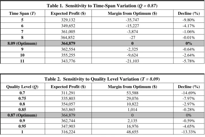
For sensitivity analysis, first Q is fixed at QOPT _{= 0.87 and the effect of T variation is illustrated in Table 1. Within a range of ~1} year from the TOPT_{, profitability decline stays within ~1 percent. Within a range of ~2 years, the decline is less than 5 percent,} and within a range of ~3 years, the decline is less than 10 percent. Second, T is fixed at TOPT _{= 8.09 and the effect Q variation} is illustrated in Table 2. Within Q range of [0.85, 0.9], the profitability decline is less than 1 percent. Within a range of [0.8, 0.95], the decline is less than 5 percent, but within a range of [0.75, 1] the decline exceeds 10 percent. The optimal solution appears to be fairly robust. Keeping T and Q, within a reasonable range around the optimum yields a relatively small deviation from optimal profitability.

Table 1. Sensitivity to Time-Span Variation (

Q = 0.87

)

Time Span (T) Expected Profit ($) Margin from Optimum ($) Decline (%)

5 329,132 -35,747 -9.80% 6 349,652 -15,227 -4.17% 7 361,005 -3,874 -1.06% 8 364,852 -27 -0.01% 8.09 (Optimum) 364,879 0 0% 9 362,554 -2,325 -0.64% 10 355,255 -9,624 -2.64% 11 343,776 -21,103 -5.78%

Table 2. Sensitivity to Quality Level Variation (

T = 8.09

)

Quality Level (Q) Expected Profit ($) Margin from Optimum ($) Decline (%)

0.7 311,291 53,588 -14.69% 0.75 335,803 29,076 -7.97% 0.8 354,057 10,822 -2.97% 0.85 363,865 1,014 -0.28% 0.87 (Optimum) 364,879 0 0% 0.9 362,744 2,135 -0.59% 0.95 347,903 16,976 -4.65% 1 316,224 48,655 -13.33%

Optimizing of the Field Structure

Potential closed-form solutions for optimal field structure were not explored in this study. However, optimization that considers field structure together with T and Q, (17), can be numerically obtained with the appropriate software.

Illustrative Example 2: The same firm considers enhancing its customer list with external information that can support additional decision tasks. The candidate enhancements are

1. Marital status 2. Number of children 3. Years of education

4. Neighborhood ranking 5. Credit status 6. Value of houses owned

7. Value of cars owned 8. Value of appliances owned

Four decision tasks are evaluated, each with a different potential value contribution and a different set of additional fields required. 1. Task 1 has a value potential of $1,000,000, and requires fields (1), (2), (3) and (5).

2. Task 2 has a value potential of $1,000,000, and requires fields (1), (2), (3) and (6). 3. Task 3 has a value potential of $200,000, and requires fields (1), (2), (4) and (7). 4. Task 4 has a value potential of $200,000, and requires fields (1), (2), (4) and (8).

Value has time sensitivity factor of 0.25 and quality sensitivity factor of 2. The fixed cost of enhancement is $100,000, plus $10,000 per field added. The per-record linear cost has a fixed component of $0.2, plus $0.1 per field added. The per-record quality cost has a fixed component of $10, plus $2 per record added. To optimize profit, the following questions need addressing: (1) Which field, among the candidates, should be added to the dataset? (2) How many years of data should be included? (3) What data quality level should be targeted?

• From the illustrative example 1: R = 10,000, * = 5, and 2 = 0.

• I = 4, since four tasks are considered. k₁ = k₂ = $1,000,000, and k₃ = k₄ = $200,000.

• {"i = 0.25}i = 1..4, the value sensitivity to time, and {$i = 2}i = 1..4, the sensitivity to quality level. • Fixed cost components: cf

0 _{= $100,000, c} f

m _{= $10,000.} • Linear cost components: cl

0 _{= $0.2, c}

l

m _{= $0.1.}

• Quality cost components: c_q0 _{= $10, c} q

m _{= $2.}

• {0_im_{}, the sensitivity factors of task [i] to field [m] are presented in the following matrix:}

Task / Field m = 1 2 3 4 5 6 7 8

i = 1 1 1 1 0 1 0 0 0

2 1 1 1 0 0 1 0 0

3 1 1 0 1 0 0 1 0

4 1 1 0 1 0 0 0 1

The optimal solution can be obtained by considering (17) as the objective function.

1. Keeping TOPT _{= 8.09 and Q}OPT _{= 0.87, as previously obtained, the optimization suggests including fields (1, 2, 3, 5, 6) and} excluding (4, 7, 8), which implies that only tasks (1) and (2) will be supported since (3) and (4) depend on excluded fields. The optimal profitability is estimated to be $300,412.

2. Reoptimizing T and Q as well. The optimization here suggests the same mix of fields. However, the optimal TOPT _{= 5.85} and QOPT _{= 0.80 are now different. The estimated optimal profitability in this case is $409,361, significantly higher then the} first result.

The results make intuitive sense: the two more profitable tasks were supported with the required fields, while the two less profitable were omitted, due to a too-high additional cost.

Conclusions and Directions for Future Research

Data management is important to business firms. While today it is driven by technical and functional efficiency, a stronger inclusion of the economic perspective is encouraged. This study suggests that data management ought to align with profit-maximization goals, and contributes to this suggestion with the proposed profit-profit-maximization framework. The framework maps the impartial/technical characteristics to the implementation costs and to the value created within contextual usage. Bringing those aspects together allows profit maximization through optimal configuration of the characteristics. The framework provides a powerful tool, from a business perspective, by consolidating value and cost; it allows trade-off assessments toward profit maximization. From the technical perspective, it informs the design of data management systems by attributing value, cost, and profitability to impartial characteristics. The framework is demonstrated through optimization of an IP with a tabular data struc-ture. The model illustrates cost/benefit trade-offs with key tabular dataset design characteristics: the time span, the quality level, and the field structure. As demonstrated, more is not necessarily better: increasing the number of records, adding more fields, and approaching perfect quality may have functional and technical merits, but may not necessarily be optimal for profitability. This study offers a range of opportunities for future research. Some are specific to the microeconomic framework proposed, while others take a broader theoretical perspective. The microeconomic model allows many possible extensions, as discussed earlier. Improving its contribution and usability requires identifying influential design characteristics, modeling their cost/benefit effect, and assessing profit optimization accordingly. Such modeling will be challenging given the issues with nonlinearity, complex constraints, stochastic behavior, considerations of current versus future goals, and dynamic behavior. For this reason, obtaining a linear-programming formulation or closed-form solutions is not likely. Alternatively, more advanced methods such as nonlinear optimization, mixed-integer programming, dynamic programming, conjoint analysis, or the real-option approach can be examined. Microeconomic modeling is applied within academic disciplines other than IS and the profitability framework could benefit from better synergy with these. Two such bodies of research are referenced here. First is the product design, which uses micro-economic models to optimize products, services, and production lines. Profit optimization of the DMP/IP coincides with the kind of problems addressed by product design research, hence, the models and analytical methods that have been proposed may be applicable to the IS/IT setting. The second body of research is data mining in which microeconomic models are applied to

value-directed information search in large datasets. Such models can contribute to a better explanation of the utility obtained from data consumption, an important part of the profitability framework that has not been sufficiently explored by IS research.

Empirical studies can help assess the value and cost associated with integrating data within business processes. Quantifying those factors can be challenging; processes are complex and involve complementary resources (Davern and Kauffman 2000). This may require exploring techniques for business process mapping and value attribution. Empirical studies can also help identify the more influential characteristics in complex systems, so that modeling can focus on a limited, but important, input set of characteristics. Another aspect to be empirically confirmed is the assumed functional forms for value and cost mapping and the calibration of their parameters.

Data management ought to be linked more robustly to the economic view of IS/IT. Data management technologies are broadly researched, and so are information value and information economics. However, value and profitability are rarely addressed in the context of data management, and technological characteristics of data management are not commonly discussed in information economics or information value research. This gap can be redressed by understanding the value contribution of data and how gains are affected by technological characteristics. A possible approach is to develop a data valuation taxonomy, identifying aspects of value contribution, detecting factors that appear to have strong explanatory power, and modeling the value contribution along those factors. Factors that appear to influence IS/IT value in a broader context often align along the distinction between the operational and the strategic: internal use versus external managerial scope (West and Courtney 1993), current versus future goals (Davern and Kauffman 2000), and uncertainty level (Sulganik and Zilcha 1996).

Finally, design for value and profitability is important not only to data management, but to system design in a broader sense. Although in recent years the economic aspects of IS (cost, value, and profitability) have drawn significant attention, it is hard to detect the influence of these concepts in IS design. This may contribute to the often-heard arguments of misalignment and disconnect between business goals and IT. The suggested framework brings the economic considerations to the forefront as goals that ought to direct optimal technical design. Such an approach, if proven to be useful, can better inform system design and architectural choices.

References

Ahituv, N. “A Systematic Approach Towards Assessing the Value of Information System,” MIS Quarterly (4:4), 1980, pp. 61-75. Arya, A., Glover, J. C., and Sivaramakrishnan, K. “The Interaction Between Decision and Control Problems and the Value of

Information,” The Accounting Review (72:4), 1997, pp. 561-574.

Ballou, D. P., and Pazer, H. L. “Designing Information Systems to Optimize the Accuracy-timeliness Tradeoff,” Information Systems Research (6:1), 1995, pp. 51-72.

Ballou, D. P., and Pazer, H. L. “Modeling Completeness versus Consistency Tradeoffs in Information Decision Systems,” IEEE Transactions fn Knowledge Management and Data Engineering (15:1), 2003, pp. 240-243.

Ballou, D. P., Wang, R., Pazer, H., and Tayi, G. K. “Modeling Information Manufacturing Systems to Determine Information Quality,” Management Science (44:4), 1998, pp. 462-484.

Banker, R. D., and Kauffman, R. J. “The Evolution of Research on Information Systems: A Fiftieth-Year Survey of the Literature in Management Science,” Management Science (50:3), 2004, pp. 281-298.

Churchman, C. W. The Design of Inquiring Systems, Basic Concepts of Systems and Organizations, Basic Books, New York, 1971.

Cooper, R., and Slugmulder, R. “Achieving Full-Cycle Cost Management,” MIT Sloan Management Review (46:1), 2004, pp. 45-52.

Davern, M. J., and Kauffman, R. J. “Discovering Potential and Realizing Value from Information Technology Investments,”

Journal of MIS (16:4), 2000, pp. 121-143.

Devaraj, S., and Kohli, R. “Performance Impacts of Information Technology: Is Actual Usage the Missing Link,” Management Science (49:3), 2003, pp. 273-289.

Easton, F. F., and Pullman, M. E. “Optimizing Service Attributes, The Seller’s Utility Problem,” Decision Sciences (32:2), 2001, pp. 251-275.

Eriksen, S. E., and Berger, P. D. “A Quadratic Programming Model for Product Configuration Optimization,” Zeitschrift für Operations Research (31:2), 1987, pp. 143-159.

Glazer, R. “Measuring the Value of Information: The Information-Intensive Organization,” IBM Systems Journal (32:1), 1993, pp. 99-110.