What to Do When
K-Means Clustering Fails:
A Simple yet Principled Alternative
Algorithm
Yordan P. Raykov1☯
*, Alexis Boukouvalas2☯
, Fahd Baig3, Max A. Little1,4
1 School of Mathematics, Aston University, Birmingham, United Kingdom, 2 Molecular Sciences, University
of Manchester, Manchester, United Kingdom, 3 Nuffield Department of Clinical Neurosciences, Oxford University, Oxford, United Kingdom, 4 Media Lab, Massachusetts Institute of Technology, Cambridge, Massachusetts, United States of America
☯These authors contributed equally to this work. *[email protected]
Abstract
The K-means algorithm is one of the most popular clustering algorithms in current use as it is relatively fast yet simple to understand and deploy in practice. Nevertheless, its use entails certain restrictive assumptions about the data, the negative consequences of which are not always immediately apparent, as we demonstrate. While more flexible algo-rithms have been developed, their widespread use has been hindered by their computa-tional and technical complexity. Motivated by these considerations, we present a flexible alternative to K-means that relaxes most of the assumptions, whilst remaining almost as fast and simple. This novel algorithm which we call MAP-DP (maximum a-posteriori Dirich-let process mixtures), is statistically rigorous as it is based on nonparametric Bayesian Dirichlet process mixture modeling. This approach allows us to overcome most of the limi-tations imposed by K-means. The number of clusters K is estimated from the data instead of being fixed a-priori as in K-means. In addition, while K-means is restricted to continuous data, the MAP-DP framework can be applied to many kinds of data, for example, binary, count or ordinal data. Also, it can efficiently separate outliers from the data. This additional flexibility does not incur a significant computational overhead compared to K-means with MAP-DP convergence typically achieved in the order of seconds for many practical prob-lems. Finally, in contrast to K-means, since the algorithm is based on an underlying statisti-cal model, the MAP-DP framework can deal with missing data and enables model testing such as cross validation in a principled way. We demonstrate the simplicity and effective-ness of this algorithm on the health informatics problem of clinical sub-typing in a cluster of diseases known as parkinsonism.
a11111
OPEN ACCESS
Citation: Raykov YP, Boukouvalas A, Baig F, Little
MA (2016) What to Do When K-Means Clustering Fails: A Simple yet Principled Alternative Algorithm. PLoS ONE 11(9): e0162259. doi:10.1371/journal. pone.0162259
Editor: Byung-Jun Yoon, Texas A&M University
College Station, UNITED STATES
Received: January 21, 2016 Accepted: August 21, 2016 Published: September 26, 2016
Copyright:©2016 Raykov et al. This is an open access article distributed under the terms of the
Creative Commons Attribution License, which
permits unrestricted use, distribution, and reproduction in any medium, provided the original author and source are credited.
Data Availability Statement: Analyzed data has
been collected from PD-DOC organizing centre which has now closed down. Researchers would need to contact Rochester University in order to access the database. For more information about the PD-DOC data, please contact: Karl D. Kieburtz, M.D., M.P.H. (https://www.urmc.rochester.edu/ people/20120238-karl-d-kieburtz).
Funding: This work was supported by Aston
research centre for healthy ageing and National Institutes of Health. The funders had no role in study design, data collection and analysis, decision to publish, or preparation of the manuscript.
1 Introduction
The rapid increase in the capability of automatic data acquisition and storage is providing a striking potential for innovation in science and technology. However, extracting meaningful information from complex, ever-growing data sources poses new challenges. This motivates the development of automated ways to discover underlying structure in data. The key infor-mation of interest is often obscured behind redundancy and noise, and grouping the data into clusters with similar features is one way of efficiently summarizing the data for further
analy-sis [1]. Cluster analysis has been used in many fields [1,2], such as information retrieval [3],
social media analysis [4], neuroscience [5], image processing [6], text analysis [7] and
bioin-formatics [8].
Despite the large variety of flexible models and algorithms for clustering available,K-means
remains the preferred tool for most real world applications [9].K-means was first introduced
as a method forvector quantizationin communication technology applications [10], yet it is
still one of the most widely-used clustering algorithms. For example, in discoveringsub-types
of parkinsonism, we observe that most studies have usedK-means algorithm to find sub-types
in patient data [11]. It is also the preferred choice in thevisual bag of wordsmodels in
auto-mated image understanding [12]. Perhaps the major reasons for the popularity ofK-means are
conceptual simplicityandcomputational scalability, in contrast to more flexible clustering
methods. Bayesian probabilistic models, for instance, require complexsampling schedulesor
variational inferencealgorithms that can be difficult to implement and understand, and are often not computationally tractable for large data sets.
For the ensuing discussion, we will use the following mathematical notation to describe
K-means clustering, and then also to introduce our novel clustering algorithm. Let us denote
the data asX= (x1,. . .,xN) where each of theNdata pointsxiis aD-dimensional vector. We
will denote thecluster assignmentassociated to each data point byz1,. . .,zN, where if data
pointxibelongs to clusterkwe writezi=k. The number of observations assigned to cluster
k, fork21,. . .,K, isNkandNkiis the number of points assigned to clusterkexcluding point
i. The parameter >0 is a small threshold value to assess when the algorithm has converged
on a good solution and should be stopped (typically= 10−6). Using this notation,K-means
can be written as in Algorithm 1.
To paraphrase this algorithm: it alternates between updating the assignments of data points
to clusters while holding the estimated clustercentroids,μk, fixed (lines 5-11), and updating the
cluster centroids while holding the assignments fixed (lines 14-15). It can be shown to find
someminimum (not necessarily theglobal, i.e. smallest of all possible minima) of the following
objective function: E¼1 2
X
K k¼1X
i:zi¼k jjxi mkjj 2 2 ð1Þwith respect to the set of all cluster assignmentszand cluster centroidsμ, where 1
2jj:jj
2
2 denotes
theEuclidean distance(distance measured as the sum of the square of differences of
coordi-nates in each direction). In fact, the value ofE cannot increaseon each iteration, so, eventually
Ewill stop changing (tested on line 17).
Perhaps unsurprisingly, the simplicity and computational scalability ofK-means comes at a
high cost. In particular, the algorithm is based on quite restrictive assumptions about the data, often leading to severe limitations in accuracy and interpretability:
Competing Interests: The authors have declared
1. By use of the Euclidean distance (algorithm line 9)K-means treats the data space asisotropic
(distances unchanged by translations and rotations). This means that data points in each
cluster are modeled as lying within aspherearound the cluster centroid. A sphere has the
same radius in each dimension. Furthermore, as clusters are modeled only by the position
of their centroids,K-means implicitly assumes all clusters have the same radius. When this
implicit equal-radius, spherical assumption is violated,K-means can behave in a
non-intui-tive way, even when clusters are very clearly identifiable by eye (see Figs1and2and
discus-sion in Sections 5.1, 5.4).
2. The Euclidean distance entails that the average of the coordinates of data points in a cluster
is the centroid of that cluster (algorithm line 15). Euclidean space islinearwhich implies
that small changes in the data result in proportionately small changes to the position of the
cluster centroid. This is problematic when there areoutliers, that is, points which are
unusu-ally far away from the cluster centroid by comparison to the rest of the points in that cluster.
Such outliers can dramatically impair the results ofK-means (seeFig 3and discussion in
Section 5.3).
3. K-means clusters data points purely on their (Euclidean)geometric closenessto the cluster
centroid (algorithm line 9). Therefore, it does not take into account the differentdensitiesof
each cluster. So, becauseK-means implicitly assumes each cluster occupies the same volume
Table 1.
Algorithm 1: K-means Algorithm 2: MAP-DP(spherical Gaussian) Input x1,. . ., xN: D-dimensional data
>0: convergence threshold K: number of clusters x1,. . ., xN: D-dimensional data >0: convergence threshold N0: prior count ^
s2: spherical cluster variance
s2
0: prior centroid variance
μ0: prior centroid location
Output z1,. . ., zN: cluster assignments μ1,. . .,μK: cluster centroids
z1,. . ., zN: cluster assignments
K: number of clusters
1 Setμkfor all k21,. . ., K 1 K = 1, zi= 1 for all i21,. . ., N
2 Enew=1 2 Enew=1
3 repeat 3 repeat
4 Eold= Enew 4 Eold= Enew
5 for i21,. . ., N 5 for i21,. . ., N 6 for k21,. . ., K 6 for k21,. . ., K 7 7 si k ¼ 1 s2 0þ 1 ^ s2Nki 1 8 8 mi k ¼ski m0 s2 0 þ 1 ^ s2 P j:zj¼k;j6¼ixj 9 di;k¼ 1 2jjxi mkjj 2 2 9 di;k¼ 1 2ðsi kþs^ 2Þjjxi m i kjj 2 2þ D 2lnðs i k þs^ 2Þ 10 10 di;Kþ1¼ 1 2ðs2 0þs^ 2Þjjxi m0jj 2 2þ D 2lnðs 2 0þs^ 2Þ 11 zi¼arg mink21;...;Kdi;k 11 zi¼arg mink21;...;Kþ1½di;k lnNki
12 12 if zi= K + 1 13 13 K = K + 1 14 for k21,. . ., K 14 15 mk¼ 1 Nk P j:zj¼kxj 15 16 E new¼ PK k¼1 P i:zi¼kdi;k 16 E new¼ XK k¼1 X i:zi¼kdi;k KlnN0 XK k¼1 logGðNkÞ 17 until Eold−Enew< 17 until Eold−Enew<
in data space, each cluster must contain the same number of data points. We will show later
that even when all other implicit geometric assumptions ofK-means are satisfied, it will fail
to learn a correct, or even meaningful, clustering when there are significant differences in
cluster density (seeFig 4and Section 5.2).
4. The numberKof groupings in the data is fixed and assumed known; this is rarely the case
in practice. Thus,K-means is quite inflexible and degrades badly when the assumptions
upon which it is based are even mildly violated by e.g. a tiny number of outliers (seeFig 3
and discussion in Section 5.3).
Some of the above limitations ofK-means have been addressed in the literature. Regarding
outliers, variations ofK-means have been proposed that use more “robust” estimates for the
cluster centroids. For example, theK-medoidsalgorithm uses the point in each cluster which is
most centrally located. By contrast, inK-mediansthe median of coordinates of all data points
in a cluster is the centroid. However, both approaches are far more computationally costly than
K-means.K-medoids, requires computation of a pairwise similarity matrix between data points
which can be prohibitively expensive for large data sets. InK-medians, the coordinates of
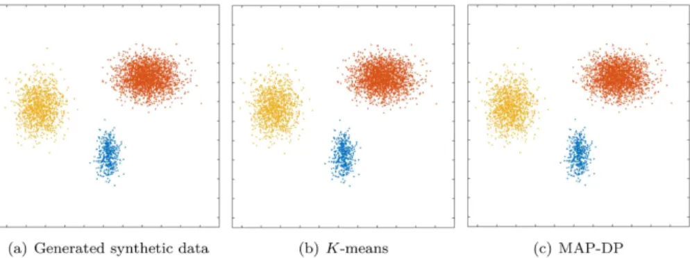
Fig 1. Clustering performed by K-means and MAP-DP for spherical, synthetic Gaussian data, with unequal cluster radii and density. The clusters are well-separated. Data is equally distributed across
clusters. Here, unlike MAP-DP, K-means fails to find the correct clustering. Instead, it splits the data into three equal-volume regions because it is insensitive to the differing cluster density. Different colours indicate the different clusters.
doi:10.1371/journal.pone.0162259.g001
Fig 2. Clustering solution obtained by K-means and MAP-DP for synthetic elliptical Gaussian data.
All clusters share exactly the same volume and density, but one is rotated relative to the others. There is no appreciable overlap. K-means fails because the objective function which it attempts to minimize measures the true clustering solution as worse than the manifestly poor solution shown here.
cluster data points in each dimension need to be sorted, which takes much more effort than computing the mean.
Provided that a transformation of the entire data space can be found which “spherizes” each
cluster, then the spherical limitation ofK-means can be mitigated. However, for most
situa-tions, finding such a transformation will not be trivial and is usually as difficult as finding the
clustering solution itself. Alternatively, by using theMahalanobis distance,K-means can be
Fig 3. Clustering performed by K-means and MAP-DP for spherical, synthetic Gaussian data, with outliers. All clusters have the same radii and density. There are two outlier groups with two outliers in each
group. K-means fails to find a good solution where MAP-DP succeeds; this is because K-means puts some of the outliers in a separate cluster, thus inappropriately using up one of the K = 3 clusters. This happens even if all the clusters are spherical, equal radii and well-separated.
doi:10.1371/journal.pone.0162259.g003
Fig 4. Clustering performed by K-means and MAP-DP for spherical, synthetic Gaussian data. Cluster
radii are equal and clusters are well-separated, but the data is unequally distributed across clusters: 69% of the data is in the blue cluster, 29% in the yellow, 2% is orange. K-means fails to find a meaningful solution, because, unlike MAP-DP, it cannot adapt to different cluster densities, even when the clusters are spherical, have equal radii and are well-separated.
adapted to non-spherical clusters [13], but this approach will encounter problematic computa-tional singularities when a cluster has only one data point assigned.
Addressing the problem of the fixed number of clustersK, note that it is not possible to
chooseKsimply by clustering with a range of values ofKand choosing the one which
mini-mizesE. This is becauseK-means isnested: we can always decreaseEby increasingK, even
when the true number of clusters is much smaller thanK, since, all other things being equal,
K-means tries to create an equal-volume partition of the data space. Therefore, data points find
themselves ever closer to a cluster centroid asKincreases. In the extreme case forK=N(the
number of data points), thenK-means will assign each data point to its own separate cluster
andE= 0, which has no meaning as a “clustering” of the data. Various extensions toK-means
have been proposed which circumvent this problem byregularizationoverK, e.g.Akaike(AIC)
orBayesian information criteria(BIC), and we discuss this in more depth in Section 3).
So far, we have presentedK-means from a geometric viewpoint. However, it can also be
profitably understood from a probabilistic viewpoint, as a restricted case of the (finite)
Gauss-ian mixture model(GMM). This is the starting point for us to introduce a new algorithm
which overcomes most of the limitations ofK-means described above.
This new algorithm, which we callmaximum a-posteriori Dirichlet processmixtures
(MAP-DP), is a more flexible alternative toK-means which can quickly provide interpretable
clustering solutions for a wide array of applications.
By contrast toK-means, MAP-DP can perform cluster analysis without specifying the
num-ber of clusters. In order to modelKwe turn to a probabilistic framework whereKgrows with the
data size, also known asBayesian non-parametric(BNP) models [14]. In particular, we use
Dirichlet process mixture models(DP mixtures) where the number of clusters can be estimated from data. To date, despite their considerable power, applications of DP mixtures are somewhat
limited due to the computationally expensive and technically challenging inference involved [15,
16,17]. Our new MAP-DP algorithm is a computationally scalable and simple way of
perform-ing inference in DP mixtures. Additionally, MAP-DP is model-based and so provides a consis-tent way of inferring missing values from the data and making predictions for unknown data.
As a prelude to a description of the MAP-DP algorithm in full generality later in the paper, we introduce a special (simplified) case, Algorithm 2, which illustrates the key similarities and
differ-ences toK-means (for the case of spherical Gaussian data with known cluster variance; in Section
4 we will present the MAP-DP algorithm in full generality, removing this spherical restriction):
• The number of clustersKis not fixed but inferred from the data. The algorithm is initialized
withK= 1 and all data points assigned to one cluster (MAP-DP algorithm line 1). In the
assignment step (algorithm line 11), a choice is made between assigning the current data
point to one of the existing clusters (algorithm line 9) or assigning it to aprior clusterlocated
atμ0with variances20(algorithm line 10). Whenskis
2
0and the current data point is the
same distance fromμ0and from the current most likely cluster centroidmki, a new cluster is
created (algorithm lines 12, 13) only if theprior count(concentration) parameterN0>Nki.
In other words, all other things being geometrically similar, only therelative countsof the
number of data points in each cluster, and the prior count, determines whether a new cluster
is created or not. By contrast, ifs i
k is very different froms
2
0, then the geometry largely
deter-mines the creation of new clusters: if a data point is closer to the prior locationμ0than to any
other most likely existing cluster centroid,m i
k , then a new cluster is created.
• In this spherical variant of MAP-DP, as withK-means, the Euclidean metric1
2jj:jj
2
2 is used
log ofN i
k is subtracted from this distance when updating assignments (algorithm line 11).
Also, the composite variances i
k þs^
2features in the distance calculations such that the
smallers i
k þs^
2
becomes, the less important the number of data points in the clusterN i
k
becomes to the assignment. In that case, the algorithm behaves much likeK-means. But, if
s i k þs^
2becomes large, then, if a cluster already has many data points assigned to it, it is
more likely that the current data point is assigned to that cluster (in other words, clusters
exhibit a “rich-get-richer” effect). MAP-DP thereby takes into account the density of clusters,
unlikeK-means. We can sees i
k þs^2as controlling the “balance” between geometry and
density.
• MAP-DP directly estimates only cluster assignments, whileK-means also finds the most
likely cluster centroids given the current cluster assignments. But, since the cluster assign-ment estimates may be significantly in error, this error will propagate to the most likely clus-ter centroid locations. By contrast, MAP-DP never explicitly estimates clusclus-ter centroids, they are treated as appropriately uncertain quantities described by a most likely cluster location
m i
k and varianceski(the centroidhyper parameters). This means that MAP-DP does not
need explicit values of the cluster centroids on initialization (K-means algorithm line 1).
Indeed, withK-means, poor choices of these initial cluster centroids can cause the algorithm
to fall into sub-optimal configurations from which it cannot recover, and there is, generally, no known universal way to pick “good” initial centroids. At the same time, during iterations
of the algorithm, MAP-DP can bypass sub-optimal, erroneous configurations thatK-means
cannot avoid. This also means that MAP-DP often converges in many fewer iterations than
K-means. As we discuss in Appendix C cluster centroids and variances can be obtained in
MAP-DP if needed after the algorithm has converged.
• The cluster hyper parameters are updated explicitly for each data point in turn (algorithm
lines 7, 8). This updating is aweighted sumofprior location μ0and the mean of the data
cur-rently assigned to each cluster. If theprior varianceparameters2
0is large or the known cluster
variances^2is small, thenμ
kis just the mean of the data in clusterk, as withK-means. By
con-trast, if the prior variance is small (or the known cluster variances^2is large), thenμ
kμ0,
the prior centroid location. So, intuitively, the most likely location of the cluster centroid is based on an appropriate “balance” between the confidence we have in the data in each cluster and our prior information about the cluster centroid location.
• WhileK-means estimates only the cluster centroids, this spherical Gaussian variant of
MAP-DP has an additional cluster variance parameter^s2, effectively determining the radius
of the clusters. If the prior variances2
0or the cluster variances^
2are small, thens i
k becomes
small. This is the situation where we have high confidence in the most likely cluster centroid
μk. If, on the other hand, the prior variances2
0is large, thenski
^
s2
N i
k . Intuitively, if we have
little trust in the prior locationμ0, the more data in each cluster, the better the estimate of the
most likely cluster centroid. Finally, for large cluster variances^2, thens i
k s
2
0, so that the
uncertainty in the most likely cluster centroid defaults to that of the prior.
A summary of the paper is as follows. In Section 2 we review theK-means algorithm and its
derivation as a constrained case of a GMM. Section 3 covers alternative ways of choosing the number of clusters. In Section 4 the novel MAP-DP clustering algorithm is presented, and the performance of this new algorithm is evaluated in Section 5 on synthetic data. In Section 6 we apply MAP-DP to explore phenotyping of parkinsonism, and we conclude in Section 8 with a summary of our findings and a discussion of limitations and future directions.
2 A probabilistic interpretation of K-means
In order to improve on the limitations ofK-means, we will invoke an interpretation which views
it as an inference method for a specific kind ofmixture model. WhileK-means is essentially
geo-metric, mixture models are inherentlyprobabilistic, that is, they involve fitting a probability
den-sity model to the data. The advantage of considering this probabilistic framework is that it
provides amathematically principledway to understand and address the limitations ofK
-means. It is well known thatK-means can be derived as an approximate inference procedure for
a special kind of finite mixture model. For completeness, we will rehearse the derivation here.
2.1 Finite mixture models
In the GMM (p. 430-439 in [18]) we assume that data points are drawn from amixture(a
weighted sum) of Gaussian distributions with densitypðxÞ ¼PKk¼1pkNðxjmk;SkÞ, whereKis
the fixed number of components,πk>0 are the weighting coefficients with
PK
k¼1pk¼1, and
μk,Skare the parameters of each Gaussian in the mixture. So, to produce a data pointxi, the
model first draws a cluster assignmentzi=k. The distribution over eachziis known as a
cate-gorical distributionwithKparametersπk=p(zi=k). Then, given this assignment, the data
point is drawn from a Gaussian with meanμziand covarianceSzi.
Under this model, the conditional probability of each data point is
pðxijzi¼kÞ ¼Nðxijmk;SkÞ, which is just a Gaussian. But an equally important quantity is the
probability we get by reversing this conditioning: the probability of an assignmentzigiven a
data pointx(sometimes called theresponsibility),p(zi=k|x,μk,Sk). This raises an important
point: in the GMM, a data point has a finite probability of belonging toeverycluster, whereas,
forK-means each point belongs to only one cluster. This is because the GMM isnota partition
of the data: the assignmentsziare treated as random draws from a distribution.
One of the most popular algorithms for estimating the unknowns of a GMM from some
data (that is the variablesz,μ,Sandπ) is theExpectation-Maximization(E-M) algorithm. This
iterative procedure alternates between theE(expectation) step and theM(maximization)
steps. The E-step uses the responsibilities to compute the cluster assignments, holding the clus-ter parameclus-ters fixed, and the M-step re-computes the clusclus-ter parameclus-ters holding the clusclus-ter assignments fixed:
E-step: Given the current estimates for the cluster parameters, compute the responsibilities:
gi;k¼p zð i¼k xj ;mk;SkÞ ¼ pkNðxijmk;SkÞ PK j¼1pjN xi mj;Sj ð2Þ
M-step: Compute the parameters that maximize thelikelihoodof the data setp(X|π,μ,S,z),
which is the probability of all of the data under the GMM [19]:
p Xð jp;m;S;zÞ ¼Y N i¼1 XK k¼1 pkNðxijmk;SkÞ ð3Þ
Maximizing this with respect to each of the parameters can be done in closed form:
Sk¼ PN i¼1gi;k pk¼ Sk N mk¼ 1 Sk XN i¼1gi;kxi Sk¼ 1 Sk XN i¼1gi;kðxi mkÞðxi mkÞ T ð4Þ
Each E-M iteration is guaranteed not to decrease the likelihood functionp(X|π,μ,S,z). So,
as withK-means, convergence is guaranteed, but not necessarily to the global maximum of the
likelihood. We can, alternatively, say that the E-M algorithm attempts to minimize the GMM objective function: E¼ XN i¼1 lnX K k¼1 pkNðxijmk;SkÞ ð5Þ
When changes in the likelihood are sufficiently small the iteration is stopped.
2.2 Connection to K-means
We can derive theK-means algorithm from E-M inference in the GMM model discussed
above. Consider a special case of a GMM where the covariance matrices of the mixture
compo-nents are spherical and shared across compocompo-nents. That meansSk=σIfork= 1,. . .,K, whereI
is theD×Didentity matrix, with the varianceσ>0. We will also assume thatσis a known
constant. Then the E-step above simplifies to:
gi;k¼ pkexp 1 2skxi mkk 2 2 PK j¼1pjexp 1 2skxi mjk 2 2 ð6Þ
The M-step no longer updates the values forSkat each iteration, but otherwise it remains
unchanged.
Now, let us further consider shrinking the constant variance term to 0:σ!0. At this limit,
the responsibility probabilityEq (6)takes the value 1 for the component which is closest toxi.
That is, of course, the component for which the (squared) Euclidean distance1
2jjxi mkjj 2 2is
minimal. So, all other components have responsibility 0. Also at the limit, the categorical
prob-abilitiesπkcease to have any influence. In effect, the E-step of E-M behaves exactly as the
assignment step ofK-means. Similarly, sinceπkhas no effect, the M-step re-estimates only the
mean parametersμk, which is now just the sample mean of the data which is closest to that
component.
To summarize, if we assume a probabilistic GMM model for the data with fixed, identical
spherical covariance matrices across all clusters and take the limit of the cluster variancesσ!0,
the E-M algorithm becomes equivalent toK-means. This has, more recently, become known as
thesmall variance asymptotic(SVA) derivation ofK-means clustering [20].
3 Inferring K, the number of clusters
The GMM (Section 2.1) and mixture models in their full generality, are a principled approach to modeling the data beyond purely geometrical considerations. As such, mixture models are useful
in overcoming the equal-radius, equal-density spherical cluster limitation ofK-means.
Never-theless, it still leaves us empty-handed on choosingKas in the GMM this is a fixed quantity.
The choice ofKis a well-studied problem and many approaches have been proposed to
address it. As discussed above, theK-means objective functionEq (1)cannot be used to select
Kas it will always favor the larger number of components. Probably the most popular approach
is to runK-means with different values ofKand use a regularization principle to pick the best
K. For instance in Pelleg and Moore [21], BIC is used. Bischof et al. [22] useminimum
descrip-tion length(MDL) regularization, starting with a value ofKwhich is larger than the expected
description length are minimal. By contrast, Hamerly and Elkan [23] suggest startingK-means with one cluster and splitting clusters until points in each cluster have a Gaussian distribution. An obvious limitation of this approach would be that the Gaussian distributions for each
clus-ter need to be spherical. In Gao et al. [24] the choice ofKis explored in detail leading to the
deviance information criterion(DIC) as regularizer. DIC is most convenient in the probabilistic
framework as it can be readily computed usingMarkov chain Monte Carlo(MCMC). In
addi-tion, DIC can be seen as a hierarchical generalization of BIC and AIC.
All these regularization schemes consider ranges of values ofKand must perform
exhaus-tive restarts for each value ofK. This increases the computational burden. By contrast, our
MAP-DP algorithm is based on a model in which the number of clusters is just another
ran-dom variable in the model (such as the assignmentszi). So,Kis estimated as an intrinsic part of
the algorithm in a more computationally efficient way.
As argued above, the likelihood function in GMMEq (3)and the sum of Euclidean
dis-tances inK-meansEq (1)cannot be used to compare the fit of models for differentK, because
this is an ill-posed problem that cannot detect overfitting. A natural way to regularize the GMM is to assume priors over the uncertain quantities in the model, in other words to turn to
Bayesian models. Placing priors over the cluster parameters smooths out the cluster shape and
penalizes models that are too far away from the expected structure [25]. Also, placing a prior
over the cluster weights provides more control over the distribution of the cluster densities.
The key in dealing with the uncertainty aboutKis in the prior distribution we use for the
clus-ter weightsπk, as we will show.
In MAP-DP, instead of fixing the number of components, we will assume that the more data we observe the more clusters we will encounter. For many applications this is a reasonable assumption; for example, if our aim is to extract different variations of a disease given some measurements for each patient, the expectation is that with more patient records more sub-types of the disease would be observed. As another example, when extracting topics from a set of documents, as the number and length of the documents increases, the number of topics is also expected to increase. When clustering similar companies to construct an efficient financial portfolio, it is reasonable to assume that the more companies are included in the portfolio, a larger variety of company clusters would occur.
Formally, this is obtained by assuming thatK! 1asN! 1, but withKgrowing more
slowly thanNto provide a meaningful clustering. But, for any finite set of data points, the
num-ber of clusters is always some unknown but finiteK+that can be inferred from the data. The
parametrization ofKis avoided and instead the model is controlled by a new parameterN0
called theconcentration parameterorprior count. This controls the rate with whichKgrows
with respect toN. Additionally, because there is a consistent probabilistic model,N0may be
estimated from the data by standard methods such as maximum likelihood and cross-valida-tion as we discuss in Appendix F.
4 Generalized MAP-DP algorithm
Before presenting the model underlying MAP-DP (Section 4.2) and detailed algorithm (Section
4.3), we give an overview of a key probabilistic structure known as theChinese restaurant
pro-cess(CRP). The latter forms the theoretical basis of our approach allowing the treatment ofKas
an unbounded random variable.
4.1 The Chinese restaurant process (CRP)
In clustering, the essential discrete, combinatorial structure is apartitionof the data set into a
parametrized by the prior count parameterN0and the number of data pointsN. For a partition
example, let us assume we have data setX= (x1,. . .,xN) of justN= 8 data points, one particular
partition of this data is the set {{x1,x2}, {x3,x5,x7}, {x4,x6}, {x8}}. In this partition there are
K= 4 clusters and the cluster assignments take the valuesz1=z2= 1,z3=z5=z7= 2,z4=z6= 3
andz8= 4. So, we can also think of the CRP as a distribution over cluster assignments.
The CRP is often described using the metaphor of a restaurant, with data points corre-sponding to customers and clusters correcorre-sponding to tables. Customers arrive at the restaurant one at a time. The first customer is seated alone. Each subsequent customer is either seated at one of the already occupied tables with probability proportional to the number of customers
already seated there, or, with probability proportional to the parameterN0, the customer sits at
a new table. We usekto denote a cluster index andNkto denote the number of customers
sit-ting at tablek. With this notation, we can write the probabilistic rule characterizing the CRP:
pðcustomeriþ1joins tablekÞ ¼
Nk N0þi if k is an existing table N0 N0þi if k is a new table 8 > > > < > > > : ð7Þ
AfterNcustomers have arrived and soihas increased from 1 toN, their seating pattern
defines a set of clusters that have the CRP distribution. This partition is random, and thus the CRP is a distribution on partitions and we will denote a draw from this distribution as:
z1;. . .;zN
ð Þ CRPðN0;NÞ ð8Þ
Further, we can compute the probability over all cluster assignment variables, given that they are a draw from a CRP:
p zð 1;. . .;zNÞ ¼ NK 0 N0ð ÞN YK k¼1 Nk 1 ð Þ! ð9Þ
whereN0ðNÞ¼N0ðN0þ1Þ ðN0þN 1Þ. This probability is obtained from a product
of the probabilities inEq (7). If there are exactlyKtables, customers have sat on a new table
exactlyKtimes, explaining the termNK
0 in the expression. The probability of a customer sitting
on an existing tablekhas been usedNk− 1 times where each time the numerator of the
corre-sponding probability has been increasing, from 1 toNk− 1. This is how the term
QK
k¼1ðNk 1Þ!
arises. TheN0ðNÞis the product of the denominators when multiplying the probabilities from
Eq (7), asN= 1 at the start and increases toN− 1 for the last seated customer.
Notice that the CRP issolelyparametrized by the number of customers (data points)Nand
the concentration parameterN0that controls the probability of a customer sitting at a new,
unlabeled table. We can see that the parameterN0controls the rate of increase of the number
of tables in the restaurant asNincreases. It is usually referred to as the concentration parameter
because it controls the typical density of customers seated at tables.
We can think of there being an infinite number of unlabeled tables in the restaurant at any given point in time, and when a customer is assigned to a new table, one of the unlabeled ones is chosen arbitrarily and given a numerical label. We can think of the number of unlabeled
tables asK, whereK! 1and the number of labeled tables would be some random, but finite
4.2 The underlying probabilistic model
First, we will model the distribution over the cluster assignmentsz1,. . .,zNwith a CRP (in fact,
we can derive the CRP from the assumption that the mixture weightsπ1,. . .,πKof the finite
mixture model, Section 2.1, have aDP prior; see Teh [26] for a detailed exposition of this
fasci-nating and important connection). We will also place priors over the other random quantities
in the model, the cluster parameters. We will restrict ourselves to assumingconjugate priorsfor
computational simplicity (however, this assumption is not essential and there is extensive
liter-ature on using non-conjugate priors in this context [16,27,28]).
As we are mainly interested in clustering applications, i.e. we are only interested in the
clus-ter assignmentsz1,. . .,zN, we can gain computational efficiency [29] byintegrating outthe
cluster parameters (this process of eliminating random variables in the model which are not of
explicit interest is known asRao-Blackwellization[30]). The resulting probabilistic model,
called theCRP mixture modelby Gershman and Blei [31], is:
z1;. . .;zN
ð Þ CRPðN0;NÞ
xi f yzi
ð10Þ
whereθare the hyper parameters of thepredictive distribution f(x|θ). Detailed expressions for
this model for some different data types and distributions are given in (S1 Material). To
sum-marize: we will assume that data is described by some randomK+number of predictive
distri-butions describing each cluster where the randomness ofK+is parametrized byN0, andK+
increases withN, at a rate controlled byN0.
4.3 MAP-DP algorithm
Much asK-means can be derived from the more general GMM, we will derive our novel
clus-tering algorithm based on the modelEq (10)above. The likelihood of the dataXis:
p Xð ;zjN0Þ ¼ p zð 1;. . .;zNÞ YN i¼1 YK k¼1 f xijy i k dz i;k ð Þ ð11Þ
whereδ(x,y) = 1 ifx=yand 0 otherwise. The distributionp(z1,. . .,zN) is the CRPEq (9). For
ease of subsequent computations, we use the negative log ofEq (11):
E¼ X K k¼1 X i:zi¼k lnf xijy i k K lnN0 XK k¼1 lnGðNkÞ C Nð 0;NÞ ð12Þ whereC Nð 0;NÞ ¼ln GðN0Þ
GðN0þNÞis a function which depends upon onlyN0andN. This can be
omitted in the MAP-DP algorithm because it does not change over iterations of the main loop
but should be included when estimatingN0using the methods proposed in Appendix F. The
quantityEq (12)plays an analogous role to the objective functionEq (1)inK-means. We wish
to maximizeEq (11)over the only remaining random quantity in this model: the cluster
assign-mentsz1,. . .,zN, which is equivalent to minimizingEq (12)with respect toz. This
minimiza-tion is performed iteratively by optimizing over each cluster indicatorzi, holding the rest,zj:j6¼i,
fixed. This is our MAP-DP algorithm, described in Algorithm 3 below.
For each data pointxi, givenzi=k, we first update the posterior cluster hyper parameters
ykibased on all data points assigned to clusterk, but excluding the data pointxi[16]. This
for a new clusterK+ 1: di;k ¼ lnf xijy i k di;Kþ1 ¼ lnf xð ijy0Þ ð13Þ
Now, the quantitydi;k lnNkiis the negative log of the probability of assigning data point
xito clusterk, or if we abuse notation somewhat and defineNKþi1 N0, assigning instead to a
new clusterK+ 1. Therefore, the MAP assignment forxiis obtained by computing
zi ¼ arg mink21;...;;Kþ1½di;k lnNki. Then the algorithm moves on to the next data pointxi+1.
Detailed expressions for different data types and corresponding predictive distributionsfare
given in (S1 Material), including the spherical Gaussian case given in Algorithm 2.
The objective functionEq (12)is used to assess convergence, and when changes between
successive iterations are smaller than, the algorithm terminates. MAP-DP is guaranteed not
to increaseEq (12)at each iteration and therefore the algorithm will converge [25]. By contrast
to SVA-based algorithms, the closed form likelihoodEq (11)can be used to estimate hyper
parameters, such as the concentration parameterN0(see Appendix F), and can be used to
make predictions for newxdata (see Appendix D). In contrast toK-means, there exists a well
founded, model-based way to inferKfrom data.
We summarize all the steps in Algorithm 3. The issue of randomisation and how it can enhance the robustness of the algorithm is discussed in Appendix B. During the execution of both K-means and MAP-DP empty clusters may be allocated and this can effect the computa-tional performance of the algorithms; we discuss this issue in Appendix A.
For multivariate data a particularly simple form for the predictive density is to assume
inde-pendent features. This means that the predictive distributionsf(x|θ) over the data will factor
into products withMterms,fðxjyÞ ¼QmM¼1fðxmjym
Þwherexm,θmdenotes the data and
Table 2.
Algorithm 3: MAP-DP (generalized algorithm) Input x1,. . ., xN: data
>0: convergence threshold N0: prior count
θ0: prior hyper parameters
Output z1,. . ., zN: cluster assignments
K: number of clusters 1 K = 1, zi= 1 for all i21,. . ., N 2 Enew=1 3 repeat 4 Eold= Enew 5 for i21,. . ., N 6 for k21,. . ., K
7 Update cluster hyper parametersy i
k (see (S1 Material)) 8 di;k¼ lnfðxijy i kÞ 9 di,K+1=−ln f(xi|θ0) 10 zi¼arg mink21;...;Kþ1½di;k lnN i k 11 if zi= K + 1 12 K = K + 1 13 Enew¼ PK k¼1 P i:zi¼kdi;k KlnN0 PK k¼1logGðNkÞ 14 until Eold−Enew<
parameter vector for them-th feature respectively. We term this the elliptical model. Including different types of data such as counts and real numbers is particularly simple in this model as there is no dependency between features. We demonstrate its utility in Section 6 where a multi-tude of data types is modeled.
5 Study of synthetic data
In this section we evaluate the performance of the MAP-DP algorithm on six different
syn-thetic Gaussian data sets withN= 4000 points. All these experiments use multivariate normal
distribution with multivariate Student-t predictive distributionsf(x|θ) (see (S1 Material)). The
data sets have been generated to demonstrate some of the non-obvious problems with theK
-means algorithm. Comparisons between MAP-DP, K-means, E-M and the Gibbs sampler
dem-onstrate the ability of MAP-DP to overcome those issues with minimal computational and conceptual “overhead”. Both the E-M algorithm and the Gibbs sampler can also be used to overcome most of those challenges, however both aim to estimate the posterior density rather than clustering the data and so require significantly more computational effort.
The true clustering assignments are known so that the performance of the different algo-rithms can be objectively assessed. For the purpose of illustration we have generated two-dimensional data with three, visually separable clusters, to highlight the specific problems that
arise withK-means. To ensure that the results are stable and reproducible, we have performed
multiple restarts forK-means, MAP-DP and E-M to avoid falling into obviously sub-optimal
solutions. MAP-DP restarts involve a random permutation of the ordering of the data.
K-means and E-M are restarted with randomized parameter initializations. Note that the
ini-tialization in MAP-DP is trivial as all points are just assigned to a single cluster, furthermore,
the clustering output is less sensitive to this type of initialization. At the same time,K-means
and the E-M algorithm require setting initial values for the cluster centroidsμ1,. . .,μK, the
num-ber of clustersKand in the case of E-M, values for the cluster covariancesS1,. . .,SKand cluster
weightsπ1,. . .,πK. The clustering output is quite sensitive to this initialization: for theK-means
algorithm we have used the seeding heuristic suggested in [32] for initialiazing the centroids
(also known as theK-means++ algorithm); herein the E-M has been given an advantage and is
initialized with the true generating parameters leading to quicker convergence. In all of the
synthethic experiments, we fix the prior count toN0= 3 for both MAP-DP and Gibbs sampler
and the prior hyper parametersθ0are evaluated usingempirical bayes(see Appendix F).
To evaluate algorithm performance we have usednormalized mutual information(NMI)
between the true and estimated partition of the data (Table 3). The NMI between two random
variables is a measure of mutual dependence between them that takes values between 0 and 1 where the higher score means stronger dependence. NMI scores close to 1 indicate good agree-ment between the estimated and true clustering of the data.
We also test the ability of regularization methods discussed in Section 3 to lead to sensible
conclusions about the underlying number of clustersKinK-means. We use the BIC as a
repre-sentative and popular approach from this class of methods. For all of the data sets in Sections
5.1 to 5.6, we varyKbetween 1 and 20 and repeatK-means 100 times with randomized
initiali-zations. That is, we estimate BIC score forK-means at convergence forK= 1,. . ., 20 and repeat
this cycle 100 times to avoid conclusions based on sub-optimal clustering results. The theory of
BIC suggests that, on each cycle, the value ofKbetween 1 and 20 that maximizes the BIC score
is the optimalKfor the algorithm under test. We report the value ofKthat maximizes the BIC
score over all cycles.
We also report the number of iterations to convergence of each algorithm inTable 4as an
run of the corresponding algorithm and ignore the number of restarts. The Gibbs sampler was run for 600 iterations for each of the data sets and we report the number of iterations until the draw from the chain that provides the best fit of the mixture model. Running the Gibbs sam-pler for a longer number of iterations is likely to improve the fit. Due to its stochastic nature, random restarts are not common practice for the Gibbs sampler.
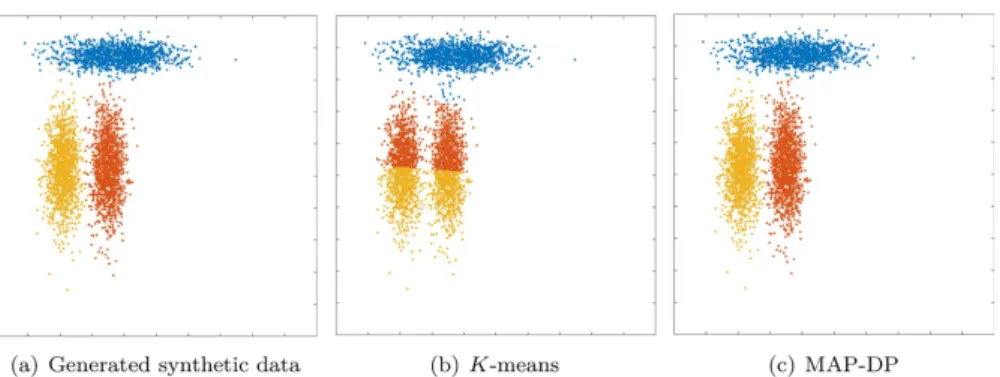
5.1 Spherical data, unequal cluster radius and density
In this example we generate data from three spherical Gaussian distributions with different
radii. The data is well separated and there is an equal number of points in each cluster. InFig 1
we can see thatK-means separates the data into three almostequal-volumeclusters. InK
-means clustering, volume is not measured in terms of the density of clusters, but rather the geo-metric volumes defined by hyper-planes separating the clusters. The algorithm does not take into account cluster density, and as a result it splits large radius clusters and merges small radius ones. This would obviously lead to inaccurate conclusions about the structure in the data. It is unlikely that this kind of clustering behavior is desired in practice for this dataset.
The poor performance ofK-means in this situation reflected in a low NMI score (0.57,
Table 3). By contrast, MAP-DP takes into account the density of each cluster and learns the
true underlying clustering almost perfectly (NMI of 0.97). This shows thatK-means can fail
even when applied to spherical data, provided only that the cluster radii are different.
Assum-ing the number of clustersKis unknown and usingK-means with BIC, we can estimate the
true number of clustersK= 3, but this involves defining a range of possible values forKand
performing multiple restarts for each value in that range. Considering a range of values ofK
between 1 and 20 and performing 100 random restarts for each value ofK, the estimated value
for the number of clusters isK= 2, an underestimate of the true number of clustersK= 3. The
highest BIC score occurred after 15 cycles ofKbetween 1 and 20 and as a result,K-means with
BIC required significantly longer run time than MAP-DP, to correctly estimateK.
Table 3. Comparing the clustering performance of MAP-DP (multivariate normal variant), K-means, E-M and Gibbs sampler in terms of NMI which has range [0, 1] on synthetic Gaussian data generated using a GMM with K = 3. NMI closer to 1 indicates better clustering.
Geometry Shared geometry? Shared population? Section NMI K-means NMI MAP-DP NMI E-M NMI Gibbs
Spherical No Yes 5.1 0.57 0.97 0.89 0.92
Spherical Yes No 5.2 0.48 0.98 0.98 0.86
Spherical Yes Yes 5.3 0.67 0.93 0.65 0.91
Elliptical No Yes 5.4 0.56 0.98 0.93 0.90
Elliptical No No 5.5 1.00 1.00 0.99 1.00
Elliptical No No 5.6 0.56 0.88 0.86 0.84
doi:10.1371/journal.pone.0162259.t003
Table 4. Number of iterations to convergence of MAP-DP, K-means, E-M and Gibbs sampling where one iteration consists of a full sweep through the data and the model parameters. The computational cost per iteration is not exactly the same for different algorithms, but it is comparable. The number
of iterations due to randomized restarts have not been included.
Section Convergence K-means Convergence MAP-DP Convergence E-M Convergence Gibbs sampler 1
5.1 6 11 10 299 5.2 13 5 21 403 5.3 5 5 32 292 5.4 15 11 6 330 5.5 6 7 21 459 5.6 9 11 7 302 doi:10.1371/journal.pone.0162259.t004
5.2 Spherical data, equal cluster radius, unequal density
In this next example, data is generated from three spherical Gaussian distributions with equal radii, the clusters are well-separated, but with a different number of points in each cluster. In
Fig 4we observe that the most populated cluster containing 69% of the data is split byK -means, and a lot of its data is assigned to the smallest cluster. So, despite the unequal density of
the true clusters,K-means divides the data into three almost equally-populated clusters. Again,
this behaviour is non-intuitive: it is unlikely that theK-means clustering result here is what
would be desired or expected, and indeed,K-means scores badly (NMI of 0.48) by comparison
to MAP-DP which achieves near perfect clustering (NMI of 0.98.Table 3). The reason for this
poor behaviour is that, if there isanyoverlap between clusters,K-means will attempt to resolve
the ambiguity by dividing up the data space into equal-volume regions. This will happen even
if all the clusters are spherical with equal radius. Again, assuming thatKis unknown and
attempting to estimate using BIC, after 100 runs ofK-means across the whole range ofK, we
estimate thatK= 2 maximizes the BIC score, again an underestimate of the true number of
clustersK= 3.
5.3 Spherical data, equal cluster radius and density, with outliers
Next we consider data generated from three spherical Gaussian distributions with equal radii and equal density of data points. However, we add two pairs of outlier points, marked as stars inFig 3. We see thatK-means groups together the top right outliers into a cluster of their own.As a result, one of the pre-specifiedK= 3 clusters is wasted and there are only two clusters left
to describe the actual spherical clusters. So,K-means merges two of the underlying clusters
into one and gives misleading clustering for at least a third of the data. For this behavior ofK
-means to be avoided, we would need to have information not only about how many groups we would expect in the data, but also how many outlier points might occur. By contrast, since
MAP-DP estimatesK, it can adapt to the presence of outliers. MAP-DP assigns the two pairs of
outliers into separate clusters to estimateK= 5 groups, and correctly clusters the remaining
data into the three true spherical Gaussians. Again,K-means scores poorly (NMI of 0.67)
com-pared to MAP-DP (NMI of 0.93,Table 3). From this it is clear thatK-means is not “robust” to
the presence of even a trivial number of outliers, which can severely degrade the quality of the clustering result. For many applications, it is infeasible to remove all of the outliers before
clus-tering, particularly when the data is high-dimensional. If we assume thatKis unknown forK
-means and estimate it using the BIC score, we estimateK= 4, an overestimate of the true
num-ber of clustersK= 3. We further observe that even the E-M algorithm with Gaussian
compo-nents does not handle outliers well and the nonparametric MAP-DP and Gibbs sampler are clearly the more robust option in such scenarios.
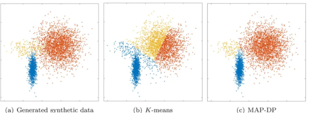
5.4 Elliptical data with equal cluster volumes and densities, rotated
So far, in all cases above the data is spherical. By contrast, we next turn to non-spherical, infact, elliptical data. This next experiment demonstrates the inability ofK-means to correctly
cluster data which is trivially separable by eye, even when the clusters have negligible overlap and exactly equal volumes and densities, but simply because the data is non-spherical and
some clusters are rotated relative to the others.Fig 2shows thatK-means produces a very
mis-leading clustering in this situation. 100 random restarts ofK-means fail to find any better
clus-tering, withK-means scoring badly (NMI of 0.56) by comparison to MAP-DP (0.98,Table 3).
In fact, for this data, we find that even ifK-means is initialized with thetruecluster
assign-ments, this is not a fixed point of the algorithm andK-means will continue to degrade the true
obtained atK-means convergence, as measured by the objective function valueEEq (1), appears to actually be better (i.e. lower) than the true clustering of the data. Essentially, for
some non-spherical data, the objective function whichK-means attempts to minimize is
funda-mentally incorrect: even ifK-means can find a small value ofE, it is solving the wrong problem.
Furthermore, BIC does not provide us with a sensible conclusion for the correct underlying
number of clusters, as it estimatesK= 9 after 100 randomized restarts.
It should be noted that in some rare, non-spherical cluster cases, global transformations of the entire data can be found to “spherize” it. For example, if the data is elliptical and all the cluster covariances are the same, then there is a global linear transformation which makes all the clusters spherical. However, finding such a transformation, if one exists, is likely at least as difficult as first correctly clustering the data.
5.5 Elliptical data with different cluster volumes, geometries and
densities, no cluster overlap
This data is generated from three elliptical Gaussian distributions with different covariances and different number of points in each cluster. In this case, despite the clusters not being
spher-ical, equal density and radius, the clusters are so well-separated thatK-means, as with
MAP-DP, can perfectly separate the data into the correct clustering solution (seeFig 5). So, for
data which is trivially separable by eye,K-means can produce a meaningful result. However, it
is questionable how often in practice one would expect the data to be so clearly separable, and indeed, whether computational cluster analysis is actually necessary in this case. Even in this
trivial case, the value ofKestimated using BIC isK= 4, an overestimate of the true number of
clustersK= 3.
5.6 Elliptical data with different cluster volumes and densities, significant
overlap
Having seen that MAP-DP works well in cases whereK-means can fail badly, we will examine
a clustering problem which should be a challenge for MAP-DP. The data is generated from three elliptical Gaussian distributions with different covariances and different number of points in each cluster. There is significant overlap between the clusters. MAP-DP manages to correctly learn the number of clusters in the data and obtains a good, meaningful solution which is close
Fig 5. Clustering solution obtained by K-means and MAP-DP for synthetic elliptical Gaussian data.
The clusters are trivially well-separated, and even though they have different densities (12% of the data is blue, 28% yellow cluster, 60% orange) and elliptical cluster geometries, K-means produces a near-perfect clustering, as with MAP-DP. This shows that K-means can in some instances work when the clusters are not equal radii with shared densities, but only when the clusters are so well-separated that the clustering can be trivially performed by eye.
to the truth (Fig 6, NMI score 0.88,Table 3). The small number of data points mislabeled by
MAP-DP are all in the overlapping region. By contrast,K-means fails to perform a meaningful
clustering (NMI score 0.56) and mislabels a large fraction of the data points that are outside
the overlapping region. This shows that MAP-DP, unlikeK-means, can easily accommodate
departures from sphericity even in the context of significant cluster overlap. As the cluster overlap increases, MAP-DP degrades but always leads to a much more interpretable solution
thanK-means. In this example, the number of clusters can be correctly estimated using BIC.
6 Example application: sub-typing of parkinsonism and
Parkinson’s disease
Parkinsonismis the clinical syndrome defined by the combination of bradykinesia (slowness of movement) with tremor, rigidity or postural instability. This clinical syndrome is most
com-monly caused byParkinson’s disease(PD), although can be caused by drugs or other conditions
such as multi-system atrophy. Because of the common clinical features shared by these other causes of parkinsonism, the clinical diagnosis of PD in vivo is only 90% accurate when com-pared to post-mortem studies. This diagnostic difficulty is compounded by the fact that PD itself is a heterogeneous condition with a wide variety of clinical phenotypes, likely driven by
different disease processes. These include wide variations in both themotor(movement, such
as tremor and gait) andnon-motorsymptoms (such as cognition and sleep disorders). While
the motor symptoms are more specific to parkinsonism, many of the non-motor symptoms associated with PD are common in older patients which makes clustering these symptoms more complex. Despite significant advances, the aetiology (underlying cause) and pathogenesis (how the disease develops) of this disease remain poorly understood, and no diseasemodifying treatment has yet been found.
The diagnosis of PD is therefore likely to be given to some patients with other causes of their symptoms. Also, even with the correct diagnosis of PD, they are likely to be affected by different disease mechanisms which may vary in their response to treatments, thus reducing the power of clinical trials. Despite numerous attempts to classify PD into sub-types using
empirical or data-driven approaches (using mainlyK-means cluster analysis), there is no
widely accepted consensus on classification.
One approach to identifying PD and its subtypes would be through appropriate clustering techniques applied to comprehensive data sets representing many of the physiological, genetic
Fig 6. Clustering solution obtained by K-means and MAP-DP for overlapping, synthetic elliptical Gaussian data. All clusters have different elliptical covariances, and the data is unequally distributed across
different clusters (30% blue cluster, 5% yellow cluster, 65% orange). The significant overlap is challenging even for MAP-DP, but it produces a meaningful clustering solution where the only mislabelled points lie in the overlapping region. K-means does not produce a clustering result which is faithful to the actual clustering.
and behavioral features of patients with parkinsonism. We expect that a clustering technique should be able to identify PD subtypes as distinct from other conditions. In that context, using
methods likeK-means and finite mixture models would severely limit our analysis as we would
need to fix a-priori the number of sub-typesKfor which we are looking. Estimating thatKis
still an open question in PD research. Potentially, the number of sub-types is not even fixed, instead, with increasing amounts of clinical data on patients being collected, we might expect a growing number of variants of the disease to be observed. A natural probabilistic model which incorporates that assumption is the DP mixture model. Here we make use of MAP-DP cluster-ing as a computationally convenient alternative to fittcluster-ing the DP mixture.
We have analyzed the data for 527 patients from thePD data and organizing center
(PD-DOC) clinical reference database, which was developed to facilitate the planning, study
design, and statistical analysis of PD-related data [33]. The subjects consisted of patients
referred with suspected parkinsonism thought to be caused by PD. Each patient was rated by a specialist on a percentage probability of having PD, with 90-100% considered as probable PD (this variable was not included in the analysis). This data was collected by several independent clinical centers in the US, and organized by the University of Rochester, NY. Ethical approval was obtained by the independent ethical review boards of each of the participating centres. From that database, we use the PostCEPT data.
For each patient with parkinsonism there is a comprehensive set of features collected through various questionnaires and clinical tests, in total 215 features per patient. The features are of different types such as yes/no questions, finite ordinal numerical rating scales, and oth-ers, each of which can be appropriately modeled by e.g. Bernoulli (yes/no), binomial (ordinal),
categorical (nominal) and Poisson (count) random variables (see (S1 Material)). For simplicity
and interpretability, we assume the different features are independent and use the elliptical model defined in Section 4.
A common problem that arises in health informatics is missing data. When usingK-means
this problem is usually separately addressed prior to clustering by some type ofimputation
method. However, in the MAP-DP framework, we can simultaneously address the problems of
clustering and missing data. In the CRP mixture modelEq (10)the missing values are treated
as an additional set of random variables and MAP-DP proceeds by updating them at every iter-ation. As a result, the missing values and cluster assignments will depend upon each other so that they are consistent with the observed feature data and each other.
We initialized MAP-DP with 10 randomized permutations of the data and iterated to
con-vergence on each randomized restart. The results (Tables5and6) suggest that the PostCEPT
data is clustered into 5 groups with 50%, 43%, 5%, 1.6% and 0.4% of the data in each cluster.
We then performed a Student’s t-test atα= 0.01 significance level to identify features that differ
significantly between clusters. As with most hypothesis tests, we should always be cautious when drawing conclusions, particularly considering that not all of the mathematical assump-tions underlying the hypothesis test have necessarily been met. Nevertheless, this analysis sug-gest that there are 61 features that differ significantly between the two larsug-gest clusters. Note
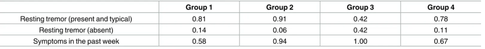
Table 5. Significant features of parkinsonism from the PostCEPT/PD-DOC clinical reference data across clusters (groups) obtained using MAP-DP with appropriate distributional models for each feature. Each entry in the table is the probability of PostCEPT parkinsonism patient answering
“yes” in each cluster (group).
Group 1 Group 2 Group 3 Group 4
Resting tremor (present and typical) 0.81 0.91 0.42 0.78
Resting tremor (absent) 0.14 0.06 0.42 0.11
Symptoms in the past week 0.58 0.94 1.00 0.67

![Table 3. Comparing the clustering performance of MAP-DP (multivariate normal variant), K-means, E-M and Gibbs sampler in terms of NMI which has range [0, 1] on synthetic Gaussian data generated using a GMM with K = 3](https://thumb-us.123doks.com/thumbv2/123dok_us/9034013.2801209/15.918.60.865.146.281/comparing-clustering-performance-multivariate-variant-synthetic-gaussian-generated.webp)