PARIS RESEARCH LABORATORY
d i g i t a l
September 1993
J ´er ˆome Barraquand
Pierre Ferbach
Path Planning
through
Variational Dynamic Programming
J ´er ˆome Barraquand
Pierre Ferbach
The authors can be contacted at the following addresses:
J´erˆome Barraquand
Digital Equipment Corporation Paris Research Laboratory 85, Avenue Victor Hugo
92500 Rueil-Malmaison, France
Pierre Ferbach ´
Ecole Nationale Sup´erieure des Techniques Avanc´ees 32, Bd Victor
75015 Paris, France
c
Digital Equipment Corporation 1994
The path planning problem, i.e., the geometrical problem of finding a collision-free path between two given configurations of a robot moving among obstacles, has been studied by many authors in recent years. Several complete algorithms exist for robots with few degrees of freedom (DOF), but they are intractable for more than 4 DOF. In order to tackle problems in higher dimensions, several heuristic approaches have been developed for various subclasses of the general problem. The most efficient heuristics rely on the construction of potential fields, attracting the robot towards its goal configuration. However, there is no obvious way to extend this approach to manipulation task planning problems.
This report presents a novel approach to path planning which does not make use of a potential function to guide the search. It is a variational technique, consisting of iteratively improving an initial path possibly colliding with obstacles. At each iteration, the path is improved by performing a dynamic programming search in a submanifold of the configuration space containing the current path. We call this method Variational Dynamic Programming (VDP). The method can solve difficult high-dimensional path planning problems without using any problem-specific heuristics. Experiments are reported for several computer simulated robots in 2D and 3D workspaces, including manipulator arms and mobile robots with up to 16 DOFs. More importantly, an extension of VDP can solve manipulation planning problems of unprecedented complexity. We report an experiment in dual-arm manipulation planning with 12 DOF in a cluttered workspace.
R ´esum ´e
Le probl`eme de la planification de trajectoire, i.e., le probl`eme g´eom´etrique consistant `a trouver des chemins sans collision entre deux configurations d’un robot en pr´esence d’obstacles, a ´et´e largement ´etudi´e ces derni`eres ann´ees. De nombreux algorithmes existent pour r´esoudre ce probl`eme dans des cas pratiques. Toutefois, l’extension de ces m´ethodes aux probl`emes de planifications de tˆaches de manipulation n’est pas triviale.
Path planning, manipulation planning, robotics, computer aided design, computer graphics, variational dynamic programming
Acknowledgements
2 Relation to other work
33 Centralized versus Distributed Representations
53.1 Definitions : : : : : : : : : : : : : : : : : : : : : : : : : : : : : : : : : 5 3.2 Centralized Representations: the Problem of Collision Detection : : : 5 3.3 Distributed Representations : : : : : : : : : : : : : : : : : : : : : : : 6
4 Variational Dynamic Programming
74.1 General VDP algorithm : : : : : : : : : : : : : : : : : : : : : : : : : : 7 4.2 Generation of the initial path : : : : : : : : : : : : : : : : : : : : : : : 8 4.3 Collision with obstacles : : : : : : : : : : : : : : : : : : : : : : : : : : 8 4.4 Generation of the repulsion points : : : : : : : : : : : : : : : : : : : : 8 4.5 Generation of the submanifolds : : : : : : : : : : : : : : : : : : : : : 9 4.6 Generation of the cost function : : : : : : : : : : : : : : : : : : : : : : 10 4.7 Generation of the minimum cost path within a submanifold : : : : : : 11 4.8 Reparameterization of the path : : : : : : : : : : : : : : : : : : : : : : 11
5 Progressive Variational Dynamic Programming
115.1 Reducing the size of the search space : : : : : : : : : : : : : : : : : 11 5.2 Progressive Variational Dynamic Programming : : : : : : : : : : : : : 12 5.3 Definition of the approximating sequence by a penalty function : : : : 14 5.4 Applications of PVDP to manipulation planning problems : : : : : : : 15
6 Experimental results
166.1 10-DOF non-serial manipulator robot in 2D workspace : : : : : : : : 16 6.2 8-DOF serial manipulator arm in 2D workspace : : : : : : : : : : : : 19 6.3 Coordination of two 3-DOF mobile robots : : : : : : : : : : : : : : : : 19 6.4 16-DOF manipulator robot in 3D workspace : : : : : : : : : : : : : : 22 6.5 A manipulation planning problem using two articulated fingers : : : : 23
7 Discussion and conclusion
231
Introduction
We present a new method for geometrical path planning with many DOF. This method, unlike other planning methods for many DOF, does not require problem-specific heuristics such as potential functions to guide the search. The method was initially developed for the basic path planning problem in open free space, but its capabilities extend to several other instances of the more general constrained motion planning problem. In particular, an extension of the method can solve complex manipulation task planning problems. It is a variational technique, consisting of iteratively improving an initial path possibly colliding with obstacles. The originality of our method is to depart from standard gradient-based variational calculus techniques. Instead, at each iteration, we perturb the current path by performing a dynamic programming search in a k-dimensional submanifold of the n-dimensional configuration space containing the current path. In practice, k is chosen equal to 2, 3, or 4 in order to make the dynamic programming search tractable. Thanks to this dynamic programming strategy, the algorithm can avoid in many cases spurious local minima of the cost functional. Furthermore, when local minima arise, the result of the dynamic programming search can be used to adequately modify the cost functional, by the introduction of additional repulsion points around colliding zones on the path. This enables the algorithm to get out of the most difficult local minima.
The k-dimensional submanifold is an arbitrarily chosen ruled surface containing the current path. This surface is quantized into a k-dimensional grid of configurations. Then, the grid is searched using Dijkstra’s algorithm with an additive cost function proportional to the number of configurations colliding with obstacles. Thus, it is guaranteed that fewer points in the new path collide with obstacles. Then, the operation is repeated until a free path is found. We call this method Variational Dynamic Programming (VDP). The idea behind VDP is to use as much as possible the power of classical complete dynamic programming-based methods, while avoiding their exponential memory and time requirements.
We have implemented this approach in a fully functional simulation program, and conducted extensive tests. Experiments are reported for several computer simulated robots in 2D and 3D workspaces, including manipulator arms and mobile robots with up to 16 DOF. To the best of our knowledge, only potential field based methods can solve problems of similar complexity. The specificity of VDP is that it can solve difficult high-dimensional planning problems without using any problem-specific heuristics. This is in itself an important point for future research in geometrical planning. It demonstrates that cluttered high-dimensional spaces can be practically searched without relying on any problem-specific knowledge. One major implication of this result is that VDP can be generalized for solving complex manipulation planning problems. This is to be contrasted with potential field based methods, which require problem-specific heuristics to resolve such problems. Of course, the generality of the method is obtained at some cost: the planner is considerably slower than some potential field-based methods, in particular the RPP method described in Barraquand and Latombe 1991 [5].
of more and more cluttered workspaces, the first being virtually free of obstacles, and the last being the original input workspace. Then, we progressively apply the VDP method to the series of workspaces. The input path used in the VDP algorithm for a given workspace in the series is the output path of the VDP method applied to the previous less cluttered workspace. In order to speed up the algorithm, the dynamic programming search at each iteration is only conducted in a small neighborhood of the current path. This makes the method considerably faster, although less general in theory. The idea is that the solution paths for two similar workspaces should be relatively close to one another in many cases. We call this version of the planner Progressive Variational Dynamic Programming (PVDP). The resulting planner is less general in theory than the original VDP planner, since it uses problem-specific heuristics to guide the search. On the other hand, it is dramatically faster. In fact, it can solve some problems in a time comparable to that of potential-field based methods.
PVDP can be used to address constrained motion planning problems, i.e., extensions of the basic path planning problem where the free space in not necessarily an open subset of the configuration space. In particular, we have successfully applied PVDP to high-dimensional manipulation planning problems. We briefly describe below the extension of the PVDP method to manipulation planning problems. A complete presentation of the method can be found in Ferbach and Barraquand 1993 [16]. Given an environment containing a robot, stationary obstacles, and movable bodies, the manipulation problem consists in finding a sequence of free robot motions, grasping and ungrasping operations, to reach a given state from a given initial state in the joint configuration space of the robot and all movable bodies. The movable objects can only move when they are grasped by the robot. The generalized obstacles (i.e., forbidden postures) in the joint configuration space C are not only the configurations where the robot or the movable objects hit the stationary obstacles, but also all postures where the movable objects are levitating without being grasped by the robot. Hence, the free space of the joint system is not anymore an open subset of the configuration space manifold. In particular, at a configuration q where the robot grasps one object, the free space in the neighborhood of q is an(n h)-dimensional submanifold of the n-dimensional configuration space C, h being the number of grasping constraints. The principle underlying PVDP is to replace the equality-constrained problem by a convergent series of more and more difficult inequality-equality-constrained planning problems in open free space. In other words, grasping constraints are handled by PVDP in an iterative fashion. PVDP first computes a path where the movable objects can levitate without being grasped by the robots. Then, this path is used as the input for a series of increasingly difficult problems where the objects must get closer and closer to the robots in order to move. The planner has successfully solved manipulation planning problems of unprecedented complexity. In particular, we report an experiment in dual-arm manipulation task planning for a 12 DOF system. Several other examples are described in Ferbach and Barraquand 1993 [16].
present experimental results illustrating the capabilities of the implemented planners. In section 7, we briefly discuss some theoretical and practical issues related to variational dynamic programming.
2
Relation to other work
The path planning problem, i.e., the geometrical problem of finding a collision-free path between two given configurations of a robot moving among obstacles, has been much studied in recent years (Latombe 1990 [24]). Today the mathematical and computational structures of the general problem (when stated in algebraic terms) are reasonably well understood (Schwartz and Sharir 1983 [32]) (Canny 1988 [11]). In addition, practical algorithms have been implemented in more or less specific cases, e.g., (Brooks and Lozano-Perez 1983 [9]) (Faverjon 1984 [14]) (Lozano-Perez [27]) (Faverjon and Tournassoud 1987 [15]) (Zhu and Latombe 1991 [35]) (Barraquand Langlois and Latombe 1992 [4] ).
Many efficient and complete algorithms exist when the number of degrees of freedom (DOF) of the robot is small (Latombe 1990 [24]): exact or approximate cell decomposition methods, roadmap methods, grid search methods. These methods differ mostly in the data representa-tions used to construct the connectivity graph of the free space. But they all rely on the same general algorithmic principle for searching the connectivity graph: Dynamic Programming. Sometimes, heuristics are imbedded to speedup the search, and various algorithms such as A or Best First Search are used instead of Breadth First algorithms such as Dijkstra’s. These algorithms nevertheless use variants of the Bellman principle of Dynamic Programming, as exemplified in Bertsekas 1988 [8]. Hence, they suffer from the traditional “curse of dimension-ality” problem of Dynamic Programming (Bellman 1958 [7]): they require exponential space and time in the number of DOF. These methods are therefore intractable for more than 4 DOF. This is not surprising, since these methods are complete, while the path planning problem is known to be PSPACE-hard.
In order to tackle problems in higher dimensions, several heuristic (i.e., incomplete) approaches have been developed for various subclasses of the general problem, and some successful systems have been implemented, e.g., (Donald 1984 [12]) and (Faverjon and Tournassoud 1987 [15]).
A widely used heuristic consists in guiding the robot along the negated gradient of a real-valued function defined over the configuration space, called the potential function. The potential has two components: a goal potential attracting the robot towards its goal configuration, and an obstacle potential, repulsing the robot from the obstacles. This so-called artificial potential
field approach was originally proposed in Khatib 1986 [20]. Emphasis was put on real-time
efficiency, rather than on completeness. In particular, since it acts as a gradient descent optimization procedure, this approach may get stuck at a local minimum of the potential function. The local-minima problem can be addressed at two levels: (1) in the definition of the
potential function, by attempting to specify a function with no or few local minima; and (2)
in the design of the search algorithm, by including appropriate techniques for escaping from local minima. At the first level, the construction of analytical potentials free of local minima has been investigated, so far with limited success. Solutions have been proposed only in Euclidean configuration spaces with spherical or star-shaped obstacles (Koditschek 1987 [21]) (Rimon and Koditschek 1989 [31]). Another line of research has been to construct numerical potential functions with “good” properties (Barraquand Langlois and Latombe 1992 [4] ). At the second level, powerful methods have been developed for escaping from local minima, in particular randomization methods (Barraquand and Latombe 1991 [5]). Very recently, new and promissing randomization methods have been developed by Overmars 1992 [30] and Kavraki and Latombe 1993 [19].
Potential field methods appear to outperform other approaches for practical path planning problems with many degrees of freedom. In particular, the RPP method described in Barraquand and Latombe 1991 [5] is already being used in industrial settings (Ohlund 1990 [29]), (Graux et al. 1992 [18]). However, the efficiency of these methods highly depends on the properties of problem-specific potential functions. In particular, extending the capabilities of potential field-based planners to more general manipulation task planning problems is a difficult task.
Our approach to manipulation task planning is fundamentally different. We do not decompose the problem into a sequence of robot motions and manipulation tasks. Our planner is not a combination of a path planner and a manipulation task planner. Instead, we simply consider the whole manipulation problem as a special instance of the basic path planning problem in the joint configuration space of the robot and the movable objects. The major advantage of this approach is to avoid the artificial decoupling between motion planning and task planning. As a consequence, PVDP can solve manipulation planning problems of unprecedented complexity.
3
Centralized versus Distributed Representations
3.1 Definitions
LetAdenote the robot,Wits workspace, andCits configuration space. A configuration of the robot, i.e., a point inC, completely specifies the position of every point inAwith respect to a coordinate system attached toW(Lozano-Perez 1983 [26]). Let n be the dimension ofC, i.e., the number of DOF. We represent a configuration q2Cby a list of n parameters(q1;:::;qn), with appropriate modulo arithmetic for the angular parameters (Latombe 1990 [24]). The subset ofCconsisting of all the configurations where the robot has no contact or intersection with the obstacles inW is called the free space and is denoted byCfree.
For each point p2A, one can consider the geometrical application that maps any configuration
q=(q1;:::;qn)2Cto the position w2W of p in the workspace. This map:
X : AC ! W
(p;q) 7! X(p;q)=w is called forward kinematic map.
3.2 Centralized Representations: the Problem of Collision Detection
practical when some objects are movable, since they may change dramatically under small displacements.
The high computational requirements of motion planning are mostly due to the need to perform repeated collision checking between the robot and the obstacles (Metivier and Urbschat 1990 [28]). Detecting the collision of a robot with many DOF in realistic environments may take as much as 1/10 to 1 second when using centralized representations. Planning of a path requires a number of collision detections ranging from a few hundred for the simplest cases to a few hundreds of thousands for the most complex ones. Such computation times are practically prohibitive for planning very complex motions using centralized representations.
3.3 Distributed Representations
The experiments reported in this paper were all performed using a distributed representation of the workspace. The workspaceWis modeled as a N-dimensional bitmap array, with N =2 or 3 being the dimension ofW. The array is defined by the following function BM:
BM : W ! f1;0g
w 7! BM(w)
in such a way that the subset of points w such that BM(w) = 1 represents the workspace obstacles and the subset of points w such that BM(w) = 0 represents the empty part of the workspace. We write:Wempty=fw2W;BM(w)=0g.
The main advantage of distributed representations is that they are structured, i.e., assessing the occupancy of any point in workspace is performed in a time constant in the number and shape of the obstacles, and in the resolution of the bitmap. A point x is occupied if and only if
BM(x)=1. Consequently, checking the collision of the robot with obstacles can be done by simply “drawing” the robot on the bitmap. The drawing procedures used are reminiscent of the Bresenham’s algorithm well known in Computer Graphics literature. Details on the collision detection methods employed can be found in (Barraquand and Latombe 1991 [5]).
4
Variational Dynamic Programming
In this section we describe the Variational Dynamic Programming (VDP) method. It is based upon a dynamic programming technique applied successively to various submanifolds of the configuration space. The idea behind VDP is to use as much as possible the power of classical complete dynamic programming-based methods, while avoiding their exponential memory and time requirements. In order to generate a free path in a configuration space of much higher dimension, VDP conducts iteratively several searches in 2 or 3-dimensional submanifolds of the configuration space.
4.1 General VDP algorithm
The input to the algorithm is:
The initial configuration qinit
The goal configuration qgoal
The specification of the forward kinematic map and the distribution of obstacles in the workspace. In the current implementation, the workspace in represented as a bitmap as described in Section 3. However, the algorithm below is independent of the chosen data representation.
The output of the algorithm at any given iteration is a path lying as much as possible in free space. The total number of iterations is arbitrarily bounded to a prespecified number. The algorithm terminates if a free path is found at a given iteration. Otherwise, the algorithm returns the best available path obtained after the prespecified number of iterations.
algorithm VDP (VARIATIONAL DYNAMIC PROGRAMMING) begin
Generation of the initial path;
while Collision with obstacles
Generation of submanifold; Generation of repulsion points; Generation of cost function;
Generation of minimum cost path within submanifold; Reparameterization of path;
endwhile; end;
This algorithm generates iteratively a series of paths joining qinit to qgoal, with a decreasing percentage of collision points.
We now describe the various parts of the general algorithm in more detail.
4.2 Generation of the initial path
In the current implementation, the initial pathis simply a geodesic path (for an appropriate metric) between (0) = qinit and (1) = qgoal in the configuration space manifold. For example, if the configuration space is a convex open subset of Rn, the initial path is the straight line joining qinitand qgoal. This straight line is quantized into a series of m+1 equally spaced configurations, the(i+1)
thpoint being
(i=m)=(1 i=m)qinit+i=mqgoal. The distance dref between two consecutive configurations is chosen small enough so as to induce a small robot motion in the workspace (see e.g., Barraquand and Latombe 1991 [5] for a discussion).
4.3 Collision with obstacles
This function returns true if the current path collides with obstacles, and false if the current path is a free path. More precisely, it examines each discrete point along the path and computes the corresponding position of the robot using the forward kinematic map. Then, it tests if this position hits obstacles using the collision detection techniques described in Section 3.
4.4 Generation of the repulsion points
At a given iteration of the VDP algorithm, the current pathcollides with obstacles at one or more points. We partition the path into a series of connected free and colliding zones. More precisely, we compute a subdivision 0 = s0 < s1 < ::: < s2r
+1
= 1 of the interval [0;1] verifying the following properties:
8i2[0;r];8s2]s2i;s2i +1
[; (s)2Cfree
8i2[0;r 1];8s2[s2i +1
;s2i +2
For each colliding zone [s2i +1
;s2i +2
], i 2 [0;r 1], we define a repulsion point rep
i =
((s2i +1
+s2i +2
)=2) in the middle of the zone. The definition of these r repulsion points will be useful for escaping local minima of the overall cost function along the path. We also compute for each repulsion point repithe radius of the corresponding colliding zone:
Ri = 1 2d((s2i
+1 );(s2i
+2 ))
where d(q;q 0
) is the Riemanian distance between q and q 0
for an appropriate metric in the configuration space manifold C. In practice, d is the Euclidean distance between the two vectors q and q0
considered as elements of Rn.
4.5 Generation of the submanifolds
We describe how a k-dimensional submanifold of the configuration space containing a given path can be constructed. At a given iteration of the VDP algorithm, we have a current path
(s)linking(0)=qinitand(1)=qgoal.
In a first step, we select two unit vectors vinit and vgoalin the generalized coordinate system
(q1;:::;qn). In the absence of reliable heuristic, we select these two vectors randomly using a uniform probability distribution on the unit sphere in Rn. We extend the path at both extremities by defining the extended path ˜in the following fashion:
˜ (s)=
8 <
:
qinit+svinit if s<0
(s) if s2[0;1]
qgoal+svgoal if s>1
In general, the extended path ˜can be defined for all s2R, i.e., it can be prolongated indefinitely in both directions. However, we assume that the configuration space is a bounded manifold. This is a very reasonable assumption, since any practical robotics system has a bounded range of action. Hence, the generalized coordinates q=(q1;:::;qn)stay in a bounded subset of R
n. Therefore, there exist two numbers smin <0 <1<smaxsuch that all configurations ˜(s)for
s 62[smin;smax]are unreachable.
In a second step, we randomly select a set of k 1 independent unit vectors u1;:::;uk 1, using again a uniform probability distribution on the unit sphere in Rn. This enables us to define parametrically a k-dimensional ruled submanifoldS
of the configuration space C:
S
=fq2C j 9(s;1;:::;k 1); q=(˜ s)+
k 1
X
i=1 iuig
As it is the case for the first parametric coordinate s, all other parametric coordinates1;:::;k 1 are bounded, since the configuration space is assumed bounded:
8i2[1;k 1]; i 2[i
min
;i
max
Hence, the set of parametric coordinates(s;1;:::;k 1) is a bounded subset of R
k. The bounded submanifoldS
is then quantized into a finite cartesian grid along its parametric co-ordinates s;1;:::;k 1, using constant incrementss;1;:::;k 1. Within the quantized submanifold, the set of neighbors of a given configuration q is the classical k-neighborhood for the parametric coordinates, i.e., the set of 3k 1 configurations whose parameters differ from those of q of one quantization step at most. For notational convenience, we will indifferently denote by s or 0 the parameter along the current path. The quantization i along each parameteriis chosen in such a way that the distance between two neighboring configurations is of the order of dref.
Remark: The construction of the k-dimensional submanifold described above can be slightly
modified in the following fashion. Instead of selecting constant unit vectors vinitand vgoal, we can select two series of “slowly” varying vectors8s<0;vinit(s)and8s>1;vgoal(s)such that the difference between two consecutive vectors in the series is “small”. Similarly, we can define slowly varying series of vectors8s;ui(s) for each index i 2 [1;k 1]. In our experiments, we have implemented both approaches. The experimental performance of the VDP algorithm does not seem to be affected by the variability of unit vectors. However, there is an important theoretical difference between the two approaches. Indeed, the version using varying unit vectors is probabilistically resolution-complete, i.e., if a solution path exists in open free space, then the probability of finding a quantized path at distance less than dref to this solution path tends towards one when the computation time tends towards infinity.
Let us assume that a collision free pathsolexists. If the unit vectors are allowed to vary along the coordinate s, it is easily seen that at each iteration, there is a very small but strictly positive lower bound p on the probability that the submanifold generated contains a path
0
identical tosolup to the configuration space quantization dref. In this event,
0
is a collision-free path in the search submanifold. The algorithm will therefore necessarily find a collision-free path thanks to the optimality of Dijkstra’s algorithm. We can conclude that the probability of finding a solution path after N iterations of VDP is lower bounded by 1 (1 p)
N. Therefore, this probability tends towards 1 when the number of iterations tends towards infinity. The rate of convergence is geometric. However, the lower bound p is so small in practice that this result says little about the actual efficiency of VDP.
4.6 Generation of the cost function
The VDP algorithm consists in iteratively improving an initial path by performing dynamic programming searches in k-dimensional submanifold grids. We describe the cost function used for the search within a given grid. The total cost along a quantized path (s0 = 0);(s1);:::;(sm=1)is an additive functional:
JC()=
m 1
X
i=0
C((si);(si +1
The elementary cost function C(q;q 0
)between two neighboring configurations is the product of two components:
C(q;q 0
)=Cobst(q;q 0
)Crep(q;q 0
)
The component Cobsthas higher values in colliding zones, thereby inducing the optimal path to lie as much as possible in free space. The component Crephas higher values in the neighborhood of repulsion points, thereby forcing the optimal path out of local minima of the pure obstacle-avoidance functional JCobst.
We now describe in more detail the expressions of Cobstand Crep.
Cobst(q;q 0
)= (
0:001
d(q;q 0
)
dref if q and q’ are non-collision configurations
1
d(q;q 0
)
dref if q or q’ is a collision configuration
where d(q;q 0
)is again the distance between q and q 0
in configuration space.
rep1;:::;rep
rbeing the r repulsion points precomputed at the current iteration, and R1;:::;Rr the radii of the corresponding colliding zones, the multiplicative cost factor Crepis defined as follows.
Crep(q;q 0
)=1+
r
X
i=1 i
Ri
d(q 00
;rep
i)
where q00 =
q+q 0
2 , and1;2;:::;rare positive coefficients chosen at each iteration randomly between 0.5 and 2 for example. We call these coefficients the repulsion coefficients.
4.7 Generation of the minimum cost path within a submanifold
This procedure achieves the dynamic programming search of an optimal path within the quantized submanifold using the standard Dijkstra’s algorithm (see e.g., Aho Hopcroft and Ullman 1983 [1]). The priority queue is implemented as a heap.
4.8 Reparameterization of the path
After an optimal path has been found by the search algorithm, the distance in configuration space between two consecutive points along the path is not equal anymore to the reference distance dref. This procedure simply reparameterizes the path in such a way that the distance between two consecutive points equals dref.
5
Progressive Variational Dynamic Programming
5.1 Reducing the size of the search space
We have found that VDP can solve all the problems that have been solved by the potential field based planner RPP (Barraquand and Latombe 1991 [5]). However, in its original form, VDP is about two orders of magnitude slower than RPP for the most difficult problems. This can be easily understood, since at each iteration of the algorithm, VDP performs an uninformed search (Dijkstra’s algorithm) of the whole k-dimensional array of quantized parametric coordinates
0;:::;k 1.
By reducing the size of this search space at each iteration, the total computation time can be dramatically reduced. Letibe the path at the end of iteration i of the VDP algorithm. If the pathiis already close to a collision free-path, the optimal pathi
+1obtained after the search of the whole k-dimensional submanifold at iteration i+1 lies in a small neighborhood ofi. Hence, a solution for dramatically reducing the number of explored cells is to limit the search fori
+1 to a small “tubular” neighborhood of
i. This will work if the configuration space is not too cluttered, i.e., if the motion planning problem at hand is simple.
In order to use the same idea for more difficult problems, a solution is to replace the initial motion planning problem by a series a simpler problems in less cluttered workspaces converging towards the initial problem. More precisely, instead of applying the VDP method directly on the input workspace, we can first generate a series of more and more cluttered workspaces using heuristic ad-hoc techniques, the first being virtually free of obstacles, and the last being the original input workspace. Then, we progressively apply the VDP method to the series of workspaces. The input path used in the VDP algorithm for a given workspace in the series is the output path of the VDP method applied to the previous less cluttered workspace. Since two consecutive problems in the series are similar, it can be expected that the solution paths for those two problems will also be similar. Hence, the dynamic programming search at each iteration can be only conducted in a small neighborhood of the current path. This idea of
Progressive Variational Dynamic Programming is described in more detail below.
5.2 Progressive Variational Dynamic Programming
Let P be our initial motion planning problem, consisting in finding a pathjoining(0)=qinit and(1)=qgoalwhile avoiding obstacles:
8s2[0;1]; (s)2Cfree
We can define in many different ways (see next subsection) a decreasing finite sequence of free-spacesC C
0
free C 1
free:::C
i
free :::C
imax
free =Cfree. Then, we can replace problem
P by the sequence of problems Pi whose solution pathsi must satisfy the simpler obstacle avoidance constraints:
8s 2[0;1]; i(s)2C
i free
The original VDP algorithm can be reparameterized to better fit the need of each subproblem
Pi.
VDP(Cfree;k;
k
max;nbiter;repulsion)
Cfree is the set of authorized configurations. k is the dimension of the submanifold where the search is conducted.
k
conducted around the current path. nbiteris the number of iterations of the VDP algorithm, i.e., the number of times a submanifold is generated and searched. repulsion is a boolean variable set totrueif the repulsion parameters have positive values,falseif they are all set to zero,
i.e., there is no repulsion.
The number
k
maxis chosen as a function of the dimension k of the submanifold. Typically, for
k =2, 2
max is chosen equal to about 8 times the size of the quantization step dref. For k =3,
3
max is chosen equal to 4dref. For k =4, 4
maxis chosen equal to dref. In other words, in a 4-dimensional submanifold, the search is only conducted along the immediate neighboring configurations of the current path.
algorithm PVDP (PROGRESSIVE VARIATIONAL DYNAMIC PROGRAMMING) begin
Generation of the initial path0using standard VDP planner;
for i=1, i<imax, i=i+1
VDP(C
i free;2;
2
max;nbiter,true); VDP(C
i free;3;
3
max;nbiter,false); VDP(C
i free;4;
4
max;nbiter,false);
ifnot foundBacktrack ;
endfor; end;
In other words, for each subproblem Pi, PVDP performs a few (nbiter)iterations of the VDP algorithm using 2D submanifolds, then performs a few iterations using 3D submanifolds, and finally continues with a few iterations using 4D submanifolds. Of course, if a free path is found to problem Piafter any of those iterations, the algorithm immediately steps to the next subproblem Pi+1. If a valid path for problem Piis not found, the algorithm backtracks, i.e., a new initial path0is generated using the standard VDP planner for problem P1, and the PVDP procedure is restarted from there.
The number nbiteris typically set to 5. The search is continued until a free pathiis found. The algorithm is stopped after a solution pathi
max = is found for the original problem. Since the algorithm may never terminate, we artificially impose an upper bound on the total running time. The algorithm returns failure if this upper bound is reached.
Remark: Instead of searching for a better path in a neighborhood of the current pathfor all
times t 2 [0;1], it is possible to limit the search locally to subintervals of[0;1]for which does not satisfy the constraints. This is how the search algorithm has been implemented in the PVDP method.
5.3 Definition of the approximating sequence by a penalty function
As described in Section 3, the obstacles in the workspace can be represented either using geometrical primitives (e.g., polygons), or using distributed representations (e.g., bitmaps). In order to define the sequence of free spacesC
i
free, we have chosen to use the representation of obstacles by geometrical primitives. Similar algorithms could be defined using bitmap representations.
We assume for the sake of simplicity that obstacles can be described as a finite set of convex polygons B1;:::;Bm. However, our approach can easily be generalized to the case of obstacles boundaries represented by higher-order polynomials. Alternatively, the obstacles could be represented through a bitmap description, and the following definition of the sequence of free spaces could be adapted accordingly.
Each face Bl
denoted gl
j. Let hjbe the number of faces of Bj. We define:
8w2W; gj(w)= min
l2[1;hj]
glj(w)
Polygon Bjcan be defined in the following way.
Bj =fw2W;gj(w)0g
Hence, a point w in the workspace does not intersect with any obstacle iff
gobst(w)= max
j2[1;m]
gj(w)<0
Besides, if the robot considered is articulated, we must check whether or not it collides with itself. We assume the set of configurations where the robot does not collide with itself can be defined by:
fq2C;gautocoll(q)<0g
Let X be the forward kinematic map of the robotA. The free spaceCfreebeing defined as the set of configurations such that the robot does not collide with itself or obstacles, we can write:
Cfree=fq2C;gautocoll(q)<0g\fq2C;8p2A;gobst(X(p;q))<0g We consider a finite decreasing sequence of numbers1 >2 >:::>i
max =0, and we define the corresponding finite sequence of free spaces
C
i
free =fq2C;gautocoll(q)<0g\fq2C;8p2A;gobst(X(p;q))<ig
The sequencei is called-strategy. More complex-strategies can be defined. For example, for a given obstacle Bj, the function gjcan be replaced by any other function g0
j:
g0
j(w)= min
l2[1;hj] ig
l j(w)
where1;:::;h
jare arbitrary positive numbers. Also, any other additional heuristic can be
added to improve the progressiveness in the sequence of problems Pi. Examples of practical
-strategies will be given in Section 6. In general we call-strategy the whole set of empirical parameters that can be used to define the sequenceC
i
free. The function gobstis called a penalty function, since it is used in the sequence of problems Pi to increasingly penalize the robot motions that do not satisfy the obstacle avoidance constraints.
5.4 Applications of PVDP to manipulation planning problems
Ferbach and Barraquand 1993 [16]. Given an environment containing a robot, stationary obstacles, and a movable object, the manipulation problem consists in finding a sequence of free robot motions, grasping and ungrasping operations, to reach a given state from a given initial state in the joint configuration space of the robot and of the movable object. The movable object can only move when it is grasped by the robot. The generalized obstacles (i.e., forbidden postures) in the joint configuration spaceCare not only the configurations where the robot or the movable object hit the stationary obstacles, but also all postures where the movable object is levitating without being grasped by the robot.
It is shown in Ferbach and Barraquand 1993 [16] that under suitable conditions on the set of stable configurations for the movable object, the grasping constraints are holonomic, i.e., they can be represented by:
8s2[0;1];ggrasp((s))=0 whereis the path followed by the robot and the movable object.
Hence, we can define in a fashion similar to that of the previous subsection a decreasing sequence of positive numbers i converging towards zero, and consider the corresponding sequence of problems Pi for which the original grasping constraint is replaced by:
8s2[0;1];ggrasp((s))<i
The principle underlying PVDP is to replace the original problem by the series of problems
Pi. In other words, grasping constraints are handled by PVDP in an iterative fashion. PVDP first computes a path where the movable objects can levitate without being grasped by the robots. Then, this path is used as the input for a series of increasingly difficult problems where the objects must get closer and closer to the robots in order to move. PVDP has successfully solved manipulation planning problems of unprecedented complexity. We report in Section 6 an experiment in dual-arm manipulation task planning for a 12 DOF system. Several other examples are described in Ferbach and Barraquand 1993 [16].
6
Experimental results
We have implemented both VDP and PVDP in two programs written in C, running on a DEC3000-500 Alpha AXP workstation. We have experimented with VDP and PVDP using a variety of robot structures. Several of these experiments are derived from the RPP simulation program developed at the Stanford Computer Science Robotics Laboratory (see e.g., Bar-raquand and Latombe 1991 [5]). We present below some of the most significant experiments, and we compare the capabilities of VDP to that of RPP.
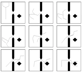
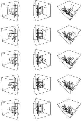
6.1 10-DOF non-serial manipulator robot in 2D workspace
Figure 1: VDP method, 2D submanifolds.
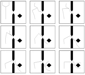
[image:25.612.148.433.384.638.2]Figure 3: PVDP method
In this example, the dimension of the submanifolds was chosen equal to k=2. The number of iterations of the VDP algorithm was 34. The total computation time was about 3 minutes. This is slower than the computation time using the RPP method, which takes about 10 seconds in this case. Using 3D submanifolds, VDP finds a path in only 3 iterations instead of 34. However, the overall computation time is over 13 minutes, since a single 3D iteration is computationally intensive. PVDP solves the same problem in less than 30 seconds. We see that the performance of PVDP is comparable to that of RPP on this relatively simple problem.
We also tested VDP on the more difficult problem depicted in Figure 2. Figure 2 shows a path found by VDP using 3D submanifolds. The number of iterations was 76, and the total computation time was 7 hours. The VDP method using only 2D submanifolds failed to solve this problem. This is dramatically slower than RPP, which solved this problem in about 30 seconds. Figure 3 shows a path found by PVDP for the same problem. The total computation time was 20 minutes. This is much faster than VDP, but still not nearly as fast as RPP.
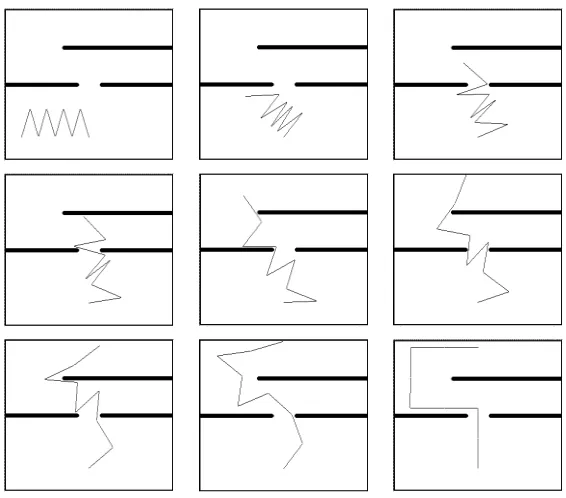
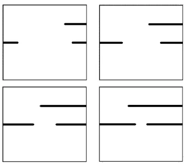
We now describe the-strategy that was used by PVDP for this problem. The original problem
P was replaced by a sequence of 15 problems Pi. Figure 4 shows a few of the workspaces in the series. The length L of the two bars in the middle was chosen according to the following formula:
8i2[1;15]; Li=L1+(L15 L1) p
i=15
A strictly similar formula was used for the diameter D of the diamond on the left. We see in the above formula that the lengths of the obstacles were increased with the square root of the problem index i, since the last steps are the most difficult.
6.2 8-DOF serial manipulator arm in 2D workspace
We consider the 8-DOF serial manipulator with 8 revolute joints depicted in Figure 5. Figure 5 shows a path found by VDP using 3D submanifolds. The number of iterations was 93. The total computation time was 6 hours. Figure 6 shows a path found by PVDP for the same problem. The computation time was 20 minutes. This is still not nearly as fast as RPP, which solved the same problem in less than 20 seconds. Figure 7 shows a few of the 40 different workspaces used in the progressive method.
6.3 Coordination of two 3-DOF mobile robots
The same planner was applied to problems requiring the coordination of two 3-DOF mobile robots in a two-dimensional workspace made of several corridors. The problem shown in figure 8 is particularly difficult because the two robots have to interchange their positions in the central corridor; hence, both of them must first move to an intermediate position in order to allow the permutation. Notice that in the initial configuration both robots are rather close to their respective goal configurations, however the paths to move there are quite long.
Figure 5: VDP method, 3D submanifolds.
[image:28.612.163.446.386.635.2]Figure 7: A few of the 40 workspaces used in the PVDP method
[image:29.612.148.433.413.599.2]PVDP in 26 minutes. This is still considerably slower than RPP, which solved this problem in less than 20 seconds.
[image:30.612.167.444.154.565.2]6.4 16-DOF manipulator robot in 3D workspace
Figure 9: 3 views of a path found by VDP for a 16DOF manipulator in a 3D workspace.
of iterations of VDP using 3D submanifolds was 20. The total computation time was 2 hours and 15 minutes. RPP solved this problem in less than 3 minutes.
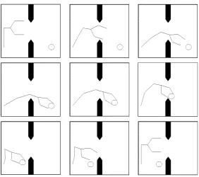
6.5 A manipulation planning problem using two articulated fingers
The 10-DOF robot depicted in Figure 1 was used in the pick and place problem illustrated in Figure 10. We used the PVDP method. The RPP planner is not designed for solving manipulation planning problems, hence cannot be compared with PVDP on this example.
The task assigned to this robot is a simple pick and place operation consisting in grasping the disk in the lower right corner of the workspace, bringing it to the lower left corner, and then returning to its initial configuration. The total number of degrees of freedom for the whole problem is 12. Figure 10 illustrates a manipulation plan found by PVDP.
In this example, the robot is said to have grasped the disk when the following conditions are satisfied:
the center M of the disk coincides with the middle R =
E1+E2
2 of the two end-effectors
E1and E2of the robot.
the distancejjE1E2jjbetween the two end effectors E1and E2is equal to the diameter D of the disk.
Let M1 and M2 be the initial and goal configurations of the disk. The grasping constraint
8t; F((t))=0 is replaced in the approximating problem P
by the constraint
8t;F((t))< with the following expression for F(q).
F(q)=min
max(jjE1E2jj D;jjRMjj); min
i2f1;2g
jjMMijj
In other words, in problem P, either the disk is at distance less than
of a docking position, or if satisfies both conditionsjjE1E2jj<D+andjjRMjj<.
The initial value ofis one fourth of the size of the workspace. Then, it is decreased at each iteration of the penalty function method by 0:001, i.e., 0:1% of the size of the workspace. The tolerance value was set totol=0:006, i.e 0:6% of the workspace. The path was computed in about half an hour.
7
Discussion and conclusion
Figure 10: A pick and place operation using a two-fingered 10-DOF robot
potential functions that make much of the power of planners such as RPP. In the current implementation of VDP, the submanifolds used for searching collision-free paths are generated purely at random. We think it should be possible to use information deriving from potential functions in order to improve the procedure generating the submanifolds. Future research will determine whether or not VDP can be made as fast as RPP through the use of numerical potential functions.
On the other hand, VDP has several unique features. First, it is a variational planner, and can therefore be used in constrained motion planning problems such as manipulation planning problems. Such problems are out of reach of classical planners such as RPP. However, as outlined in Ferbach and Barraquand 1993 [16], it may be possible to develop a variational version of RPP. Future research will determine whether a variational version of RPP can be made as efficient as PVDP for solving manipulation planning problems.
Second, VDP uses dynamic programming. This may become an important advantage over ran-domized planners when addressing motion planning problems with non-holonomic constraints. Indeed, optimal algorithms based upon dynamic programming already exist (Barraquand and Latombe 1993 [6]) for planning motions of non-holonomic mobile robots with few DOF. We think it is possible to use the main ideas underlying VDP to develop a motion planner for non-holonomic robots with many DOF. This extension is left for future research.
References
1. Aho, A.V., Hopcroft, J.E., and Ullman, J.D. Data Structures and Algorithms, Addison-Wesley (1983).
2. Alami, R., Simeon, T., and Laumond J.P. A Geometrical Approach to Planning Manipu-lation Tasks: The Case of Discrete Placements and Grasps. In Miura, H. and Arimoto, S. (editors), Robotics Research 5, MIT Press, pages 453–459 (1989).
3. Barraquand, J., Langlois, B. and Latombe, J.C. Robot Motion Planning with Many Degrees of Freedom and Dynamic Constraints. In Miura, H. and Arimoto, S. (editors), Robotics
Research 5, MIT Press, pages 435–444 (1989).
4. Barraquand, J., Langlois, B. and Latombe, J.C. Numerical Potential Field Techniques for Robot Path Planning. IEEE Transactions on Systems, Man, and Cybernetics, 22(2) (1992).
5. Barraquand, J. and Latombe, J.C. Robot Motion Planning: A Distributed Representation Approach. International Journal of Robotics Research, MIT Press, 10(6) (1991).
6. Barraquand, J. and Latombe, J.C. NonHolonomic MultiBody Mobile Robots: Controlla-bility and Motion Planning in the Presence of Obstacles. Algorithmica, 10(2/3/4) (1993).
7. Bellman, R. Dynamic Programming. Princeton University Press, Princeton (1957).
8. Bertsekas, D.P. Dynamic Programming. Deterministic and Stochastic Models Prentice-Hall, Englewood Cliffs, N.J. (1987).
9. Brooks, R.A. and Lozano-P´erez, T. A Subdivision Algorithm in Configuration Space for Find-Path with Rotation. In Proceedings of the 8th International Joint Conference on
Artificial Intelligence (Karlsruhe, FRG), pages 799–806 (1983
10. Buckley, C.E. The Application of Continuum Methods to Path Planning, Ph.D. Dissertation, Department of Mechanical Engineering, Stanford University, CA. (1985).
11. Canny, J.F. The Complexity of Robot Motion Planning. MIT Press, Cambridge, MA. (1988).
12. Donald, B.R. Motion Planning with Six Degrees of Freedom. Technical Report 791, Arti-ficial Intelligence Laboratory, MIT, Cambridge (1984).
13. Dupont, P.E., and Derby, S. An Algorithm for CAD-based Generation of Collision-Free Robot Paths. In Proceedings of NATO workshop on CAD Based Programming for Sensory
Robots (Il Ciocco, Italy), July 1988.
14. Faverjon, B. Obstacle Avoidance Using an Octree in the Configuration Space of a Manip-ulator. In Proceedings of the IEEE International Conference on Robotics and Automation
15. Faverjon, B. and Tournassoud, P. A Local Based Approach for Path Planning of Manipula-tors with a High Number of Degrees of Freedom. In Proceedings of the IEEE International
Conference on Automation and Robotics (Raleigh), pages 1152–1159 (1987).
16. Ferbach, P. and Barraquand, J. A Penalty Function Method for Constrained Motion
Plan-ning. Research report 34, Paris Research Laboratory, Digital Equipment Corp., September
1993.
17. Gilbert, E.G., and Johnson, D.W. Distance Functions and their Application to Robot Path Planning in the Presence of Obstacles. IEEE Transactions on Robotics and Automation (1985).
18. Graux, L., Millies, P., Kociemba, P.L., and Langlois, B. Integration of a Path Generation Algorithm into Off-line Programming of AIRBUS Panels. In Proceedings of Aerofast’92
(Bellevue, Washington), SAE Technical papers series , October 1992.
19. Kavraki, L. and Latombe J.C. Randomized Preprocessing of Configuration Space for Fast
Path Planning. Technical report STAN-CS-93-1490, Stanford University, September 1993.
20. Khatib, O. Real-Time Obstacle Avoidance for Manipulators and Mobile Robots.
Interna-tional Journal of Robotics Research. 5(1):90-98 (1986)
21. Koditschek, D.E. Exact Robot Navigation by Means of Potential Functions: Some Topo-logical Considerations. In Proceedings of the IEEE International Conference on Robotics
and Automation, Raleigh, pages 1–6 (1987).
22. Koga, Y. and Latombe, J.C. Experiments in Dual-Arm Manipulation Planning. In
Proceed-ings of the IEEE International Conference on Robotics and Automation (Nice, France),
pages 2238–2245, May 1992.
23. Koga, Y. and Latombe, J.C. On Multi-Arm Manipulation Planning. Working paper, Robotics Laboratory, Computer Science Department, Stanford University, 1993.
24. Latombe, J.C. Robot Motion Planning. Kluwer Academic Publishers, Boston (1990).
25. Laumond, J.P. and Alami, R. A Geometrical Approach to Planning Manipulation Tasks in
Robotics. Technical Report 89-261, LAAS, Toulouse, France (1989).
26. Lozano-P´erez, T. Spatial Planning: A Configuration Space Approach. IEEE Transactions
on Computers. C-32(2):108-120 (1983).
27. Lozano-P´erez, T. A Simple Motion-Planning Algorithm for General Robot Manipulators.
IEEE Journal of Robotics and Automation. RA-3(3):224-238 (1987).
28. M´etivier, C. and Urbschat, R. Run-Time Statistical Analysis of a Robot Motion Planning
Al-gorithm. Internal Technical Note, Robotics Laboratory, Computer Science Dept., Stanford
University (1990).
30. Overmars, M. A Random Approach to Path Planning, TR 32, Utrecht Univ., The Nether-lands, 1992.
31. Rimon, E. and Koditschek, D.E. The Construction of Analytic Diffeomorphisms for Exact Robot Navigation on Star Worlds. In Proceedings of the IEEE International Conference
on Robotics and Automation (Scottsdale), pages 21–26 (1989).
32. Schwartz, J.T. and Sharir, M. On the ‘Piano Movers’ Problem: II. General Techniques for Computing Topological Properties of Real Algebraic Manifolds. Advances in Applied
Mathematics. Academic Press, 4:298-351 (1983).
33. Warren, C.W. Global Path Planning using Artificial Potential Fields. In Proceedings IEEE
International Conference on Robotics and Automation (Washington D.C.), pages 316–321
(1989).
34. Wilfong, G. Motion Planning in the Presence of Movable Obstacles. In Proceedings of the
4th ACM Symposium of Computational Geometry, pp 279-288 (1988).