Munich Personal RePEc Archive
Dirichlet Process Hidden Markov
Multiple Change-point Model
Ko, Stanley I. M. and Chong, Terence T. L. and Ghosh,
Pulak
University of Macau, The Chinese University of Hong Kong and
Nanjing University, Indian Institute of Management at Bangalore
7 August 2014
Online at
https://mpra.ub.uni-muenchen.de/57871/
Dirichlet Process Hidden Markov Multiple Change-point
Model
∗
Stanley I.M. Ko
†Terence T.L. Chong
‡Pulak Ghosh
§August 7, 2014
Abstract
This paper proposes a new Bayesian multiple change-point model which is based on the hidden Markov approach. The Dirichlet process hidden Markov model does not require the specification of the number of change-points a priori. Hence our model is robust to model specification in contrast to the fully parametric Bayesian model. We propose a general Markov chain Monte Carlo algorithm which only needs to sample the states around change-points. Simulations for a normal mean-shift model with known and unknown variance demonstrate advantages of our approach. Two applications, namely the coal-mining disaster data and the real US GDP growth, are provided. We detect a single change-point for both the disaster data and US GDP growth. All the change-point locations and posterior inferences of the two applications are in line with existing methods.
Keywords: Change-point; Dirichlet process; Hidden Markov model; Markov chain Monte Carlo; Nonparametric Bayesian.
∗The authors would like to thank all the participants in the Econometric Society Australasian Meet-ing 2011, Adelaide, Australia, July 2011, for helpful comments and discussions. The third author (P.G.) acknowledges the support of DST grant (SR/S4/MS:648/10) from the Government of India.
†Corresponding author: Department of Finance and Business Economics, University of Macau, Macau, China. Email: [email protected].
‡Department of Economics and Institute of Global Economics and Finance, The Chinese University of Hong Kong, Hong Kong, and Department of International Eonomics and Trade, Nanjing University, China. Email: [email protected].
1
Introduction
The earliest Bayesian change-point model is explored by Chernoff and Zacks (1964), who assume a constant probability of change at each point in time. Smith (1975) investigate the single change-point model under different assumptions of model parameters. Carlin, Gelfand, and Smith (1992) assume that the structural parameters are independent of the change-points and introduce the Markov chain Monte Carlo sampling method to derive the posterior distributions. Stephens (1994) further applies the Markov chain Monte Carlo method to the case of multiple changes. Chib (1998) allows the change-point probability to depend on the regime between two adjacent change-points. Koop and Potter (2007) propose the Poisson hierarchical prior for durations in the change-point model that allows the number of points to be unknown. More recent works on the Bayesian change-point model include Wang and Zivot (2000), Giordani and Kohn (2008), Pesaran, Pettenuzzo, and Timmermann (2006), Maheu and Gordon (2008) and Geweke and Yu (2011).
In this paper we follow the modeling strategy of Chib (1998) which is one of the most pop-ular Bayesian change-point models. He introduces a discrete random variable indicating the regime from which a particular observation is drawn. Specifically, letYn= (y1, y2, . . . , yn)′ be
the observed time series, such that the density of yt conditioned on Yt−1 = (y1, y2, . . . , yt−1)′
depends on the parameterθ whose value changes at an unknown time period 1< τ1 <· · ·<
τk< n and remains constant within each regime, that is,
yt∼
p(yt|Yt−1, θ1) if t≤τ1,
p(yt|Yt−1, θ2) if τ1 < t≤τ2,
... ...
p(yt|Yt−1, θk) if τk−1 < t≤τk,
p(yt|Yt−1, θk+1) ifτk< t≤n,
(1)
where θi ∈ Rl is an l dimension vector, i = 1,2, . . . , k + 1. Note that we consider in this
paper the change-point problem when the data are assumed to be generated by a parametric
model where the unknown parameter θi changes with respect to different regimes. Let st be
the discrete indicator variable such that
yt|st∼p(yt|Yt−1, θst), (2)
wheresttakes values in{1,2, . . . , k, k+ 1}. The indicator variablest is modeled as a discrete
time, discrete-state Markov process with the constrained transition probability matrix
P =
p11 p12 0 · · · 0
0 p22 p23 · · · 0
... ... ... ... ...
... ... ... pkk pk(k+1)
0 0 · · · 0 1
where pij = pr(st = j | st−1 = i) is the probability of moving to regime j at time t given
that the regime at time t−1 isi. With this parameterization, the ith change-point occurs
atτi if sτi =i and sτi+1 =i+ 1.
As pointed out in Chib (1998), the above is a hidden Markov model where the transition
matrix of the hidden state st is restricted as in (3). Hence, Chib’s multiple change-point
model inherits the limitation of the hidden Markov model in that the number of states has to be specified in advance. In light of this, Chib (1998) suggests to select from alternative models (e.g. one change-point v.s. multiple change-points) according to the Bayes factors. In this paper, we introduce the Dirichlet process hidden Markov model (DPHMM) with left-to-right transition dynamic, without imposing restrictions on the number of hidden states. The use of the DPHMM has the following appealing features:
1. We do not have to specify the number of states a priori. The information provided
by the observations determines the states endogenously. Hence, our method can be regarded as semiparametric.
2. Our modeling approach facilitates the sampling of states since we only need to sample the states around change-points.
We note that (Kozumi and Hasegawa (2000)) propose a method similar to ours in that they
utilize a Dirichlet process prior for θ, but in a mixture model.
The rest of the paper is organized as follows. Section 2 provides a brief introduction of the Dirichlet process. Section 3 incorporates the Dirichlet process into the change-point model. The general Markov chain Monte Carlo sampler is discussed in Section 4. A Monte Carlo study of the normal mean-shift model is conducted in Section 5. Section 6.1 discusses learning of DPHMM parameters. Section 7 provides applications of our model and Section 8 concludes the paper.
2
The Dirichlet Process
Our new method employs the Dirichlet process technique which is widely used in nonpara-metric Bayesian models. The Dirichlet process prior is first proposed by Ferguson (1973). He derives the Dirichlet process prior as the prior on the unknown probability measure space
with respect to some measurable space (Ω,F). Hence the Dirichlet process is a distribution
over probability measures. Blackwell and MacQueen (1973) show that the Dirichlet process can be represented by the Polya urn model. Sethuraman (1994) develops the constructive sticking-breaking definition.
(Neal (1992), Neal (2000) and Beal, Ghahramani, and Rasmussen (2002)). To illustrate the idea, let us first consider the case with a finite number of states. With the left-to-right
restriction to the transition dynamic, a particular state st−1 = i will either stay at the
current state i or transit to a state j > i. A left-to-right Markov chain with k states will
typically have the following upper triangular transition matrix
P =
p11 p12 p13 · · · p1k
0 p22 p23 · · · p2k
0 0 p33 · · · p3k
... ... ... ... ...
0 0 · · · pkk
, (4)
where the summation of each row equals 1. Note that the left-to-right Markov chain here is
different from Chib’s restricted band transition matrix (3). Here, the number of states k is
not necessarily the number of regimes as the case in Chib’s model.
Let pi = (0, . . . , pii, pi(i+1), . . . , pik) be the transition probabilities of the ith row of the
transition matrix (4). Suppose we draw m samples {c1, . . . , cm} of st+1 given st = i with
probability profilepi. The joint distribution of the sample is thus
pr(c1, . . . , cm |pi) = k
Y
j=i
pmj
ij , (5)
where mj denotes the number of samples that take state j, j = i, . . . , k. We assume a
symmetric Dirichlet prior π(pi |β) for pi with positive concentration parameter β
pi |β ∼Dirichlet(β/(k−i+ 1), . . . , β/(k−i+ 1)) =
Γ(β)
Γ k−βi+1k−i+1
k
Y
j=i
pβ/ij(k−i+1)−1. (6)
With the Dirichlet prior, we can analytically integrate out pi such that
pr(c1, . . . , cm |β) =
Z
pr(c1, . . . , cm |pi, β)dπ(pi |β) =
Γ(β)
Γ(m+β)
k
Y
j=i
Γ mj +k−βi+1
Γ k−βi+1 . (7)
The conditional probability of a sample cd ∈ {c1, . . . , cm} given all other samples is thus
pr(cd =j |c−d) =
m−d,j +β/(k+i−1)
m−1 +β , (8)
wherec−ddenotes the sample set withcddeleted, andm−d,j is the number of samples in c−d
that take state j.
Taking the limit of equation (8) as k tends to infinity, we have
pr(cd=j |c−d) =
( m
−d,j
m−1+β j ∈ {i, i+ 1, . . . , k}, β
m−1+β for all potential states .
Note that the probability that cd takes an existing state, say j, is proportional to m−d,j,
which implies that cd is more likely to choose an already popular state. In addition, the
probability that a new state (i.e. k+ 1) takes place is proportional to β. Hence, there are
potentially many states available, with infinite dimension transition matrix
P =
p11 p12 p13 · · ·
0 p22 p23 · · ·
0 0 p33 · · ·
... ... ... ...
. (10)
The actual state space can be regarded as consisting of an infinite number of states, only a finite number of which are actually associated with the data. Therefore, the number of states is endogenously determined.
3
The Dirichlet Process Hidden Markov Multiple
Change-point Model and the State Evolution
Let us now turn to the proposed multiple change-point model and discuss a particular state
evolution. Suppose we have already generated the hidden states up to st = i. We impose
the Dirichlet process as described in Section 2 to st+1. In the change-point model, the
transitions that have existed so far from state i are only self transitions. With the
left-to-right restriction, we will neither see a backward transition, i.e., transition from state i to
some previous states, nor a forward transition, i.e., transition to some future states. The
counts of the existing transitions from state iwill be used as the counts defined in equation
(9). Hence, we will have
pr(st+1 =j |st=i, s1, . . . , st−1) = (
nii
nii+β j =i,
β
nii+β st+1 takes a new state,
(11)
where nii = Ptt−′=11 δ(st′, i)δ(st′+1, i) denotes the counts of transitions that have occurred so
far from state i to itself.1 Note that in equation (11), s
t+1 depends only on the state that
st takes according to the Markovian property. All other previous states merely provide the
transition counts.
We introduce a self-transition prior mass α for each state. The idea here is that if st
transits to a new state, say st+1 =i+ 1, then without previous transition records, the next
state st+2 conditioned on st+1 = i+ 1 will further take another new state with probability
1. Hence, with α, the trivial case is avoided and we have
pr(st+1 =j |st=i, s1, . . . , st−1) = ( n
ii+α
nii+β+α j =i,
β
nii+β+α st+1 takes a new state.
(12)
1
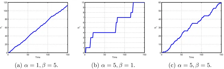
Therefore, the whole Markov chain is characterized by two parameters, α and β, instead
of a transition probability matrix. We can see that α controls the prior tendency to linger
in a state, and β controls the tendency to explore new states. Figure 1 illustrates three
left-to-right Markov chains of length n = 150 with different α and β. Figure 1a depicts the
chain that explores many new states with very short linger time. Figure 1b shows the chain with long linger time and less states. Figure 1c lies in between.
Equation (12) coincides with Chib (1998)’s model when the probability pii is integrated
out. Specifically, in Chib (1998),
pr(st+1 =j |st=i, s1, . . . , st−1)
=
Z
p(st+1=j |st=i, s1, . . . , st−1, pii)f(pii)dpii
=
( n
ii+a
nii+a+b j =i,
b
nii+a+b j =i+ 1.
(13)
where pii ∼ Beta(a, b) and f(pii) is the corresponding density. However, our model stems
from a different perspective. The derivations in the previous section and equation (12) follow the nonparametric Bayesian literature (Neal (2000)) and the infinite HMM of Beal, Ghahramani, and Rasmussen (2002). Indeed, it is known that when the Dirichlet process is truncated at a finite number of states, the process reduces to the generalized Dirichlet distribution (GDD), see Connor and Mosimann (1969) and Wong (1998). For the same reason we have (12) coincides with (13). We would like to point out that our modeling
strategy facilitates the Gibbs sampler of st which is different from Chib (1998). We will
elaborate further on the Gibbs sampler in the next section. Also, learning of α and β will
be discussed in Section 6.1.
0 50 100 150
0 20 40 60 80 100 120
Time St
(a)α= 1, β = 5.
0 50 100 150
0 1 2 3 4 5 6 7 8 9 10
Time
St
(b)α= 5, β= 1.
0 50 100 150
0 10 20 30 40 50 60
Time
St
[image:7.612.118.490.492.607.2](c) α= 5, β= 5.
4
Markov Chain Monte Carlo Algorithm
4.1
General
Suppose we have observations Yn = (y1, y2, . . . , yn)′. Given the state Sn = (s1, . . . , sn)′ we
have
yt|st∼p(yt|Yt−1, θst), (14) whereθst ∈R
l,Y
t−1 = (y1, . . . , yt−1)′. Letθ = (θ1, . . . , θk)′ andγ denotes a hyperparameter.
Recall that we impose the DPHMM to the states and a hierarchical model to the parameter, we are thus interested in sampling from the posterior p(θ, Sn, γ |Yn) given the priorsp(θ|γ),
p(γ) and p(Sn). The general Gibbs sampler procedure is to sample the following in turn:
Step 1. Sn |θ, γ, Yn,
Step 2. θ |γ, Sn, Yn,
Step 3. γ |θ, Sn, Yn.
We will discuss the three steps below.
4.2
Simulation of
S
nThe state prior p(Sn) can be easily derived from (12). Moreover, the full conditional is
p(Sn |θ, γ, Yn)∝p(Sn)p(Yn |Sn, θ, γ). (15)
Simulation of Sn from the full conditional (15) is done by the Gibbs sampler. Specifically,
we draw st in turn for t= 1,2, . . . , n from
p(st|St−1, St+1, θ, γ, Yn)∝p(st|st−1, St−2)p(st+1 |st, St+2)p(yt|st, Yt−1, θ, γ), (16)
where St−1 = (s1, . . . , st−1)′ and St+1 = (st+1, . . . , sn)′. The most recent updated values of
the conditioning variables are used in each iteration. Note that we write p(st | st−1, St−2)
andp(st+1 |st, St+2) to emphasize the Markov dynamic; the other conditioning states merely
provide the counts.
With the left-to-right characteristic of the chain, we do not have to sample all st from
t = 1 to T. Instead, we only need to sample the state in which a change-point takes place.
To see this, let us consider a concrete example. Suppose from the last sampler, we have
s1 s2 s3 s4 s5 s6 s7 s8 s9 s10 s11 · · ·
With left-to-right transition restriction, st requires a sampling from (16) if and only if st−1
and st+1 differ. For other cases, st is unchanged with probability one. Suppose we are at
t = 2. Since s1 and s3 are both equal to 1, s2 is forced to take 1. In the above chain, the
first state that needs to sample from (16) iss3, which will either take the values 1 or 2 (s2 or
s4). If s3 takes 2 in the sampling (i.e., joining the following regime), then the next state to
sample would be s5; otherwise (i.e., joining the preceding regime), the next state to sample
is s4 because s5 −s3 6= 0 for s3 = 1. Now suppose we are at t = 9. We will draw a new s9
and s9 will either join the regime of s8 or the regime ofs10. This will look strange because a
gap exists in the chain. However, our concern here is the consecutive grouping orclustering
in the series. We can alternatively think that the state represented by s9 is simply pruned
away in the current sweep. Note the numbers assigned to thest’s are nothing but indicators
of regimes.2 Therefore, we will relabel the s
t’s after each sweep.
In general, suppose st−1 = i and st+1 = i+ 1. st takes either i or i+ 1. Table 1 shows
the corresponding probability values specified in (16). To see this, if st takes i, then the
transition from st−1 to st is a self-transition and that from st to st+1 is an innovation. The
corresponding probability values are in the first row of Table 1. The reasoning forst =i+ 1
is similar. Note the changes of counts in different situations.
Table 1: Sampling probabilities ofst.
p(st |st−1 =i, St−2) p(st+1=i+ 1|st, St+2) p(yt |st, Yt−1, θ)
st =i
nii+α
nii+β+α
β
nii+ 1 +β+α
p(yt|Yt−1, θi)
st =i+ 1
β nii+β+α
ni+1,i+1+α
ni+1,i+1+β+α p(yt|Yt−1, θi+1)
Note:
nii =Ptt−′=12 δ(st′, i)δ(st′+1, i) andni+1,i+1 =
Pn−1
t′=t+1δ(st′, i+ 1)δ(st′+1, i+ 1).
For the initial point s1, if currently s2−s1 6= 0, then we can sample s1 from
pr(s1 |s2, s3, . . . , sn) =
(
c· β+αα ·β+βα ·p(y1 |Y0, θs1) if s1 unchanged,
c· β+βα · ns2s2+α
ns2s2+β+α ·p(y1 |Y0, θs2) ifs1 =s2,
(17)
wherens2s2 =
Pn−1
t′=2δ(st′, s2)δ(st′+1, s2) andcis the normalizing constant. For the end point
sn, if sn−sn−1 6= 1, we sample sn from
pr(sn |sn−1, sn−2, . . . , s1) = (
c· nsn−1sn−1+α
nsn−1sn−1+β+α ·p(yn |Yn−1, θsn−1) if sn=sn−1,
c·n β
sn−1sn−1+β+α ·p(yn |Yn−1, θsn) if sn unchanged,
(18)
where nsn−1sn−1 =
Pn−2
t′=1δ(st′, sn−1)δ(st′+1, sn−1) and cis the normalizing constant. 2
As mentioned in Section 3, the DPHMM facilitates the Gibbs sampler of states. In
sampling st from (16), we simultaneously use up all information of the transitions prior to
t (i.e. s1, . . . , st−1) and after t (i.e. st+1, . . . , sT) which are captured in p(st |st−1, St−2) and
p(st+1 |st, St+2). Thus far, our algorithm only requires a record of transitions and draws at
the point where the structural change takes place, whereas we have to sample allst in Chib
(1998).
4.3
Updating
θ
and
γ
Given Sn and Yn, the full conditionals of θ and γ are simply
p(θi |γ, Sn, Yn)∝p(θi |γ)
Y
{t:st=i}
p(yt|Yt−1, θi),
p(γ |θ, Sn, Yn)∝p(γ)p(θ |γ, Sn, Yn),
(19)
which are model specific. In the following sections, we will study a simulated normal
mean-shift model, a discrete type Poisson model, and an ar(2) model.
4.4
Initialization of states
In Section 4.2, we have discussed the simulation of the states Sn. The number of
change-points is inherently estimated through the sampling of states in equation (16). Within the burn-in period, the state number will be changing around after each MCMC pass. After the burn-in period, the Markov chain converges and hence the number of states becomes stable. Theoretically, it is legitimate to set any number of change-points in the beginning and let the algorithm find out the convergent number of states. In practice, we find it is more efficient to initialize with a large number of states and let the algorithm prune away redundant states, rather than allow for the change-point number to grow from a small number. Specifically,
suppose a reasonably large state numberk is proposed. We initialize equidistant states, that
is
st =i, if
(i−1)·n
k < t≤ i·n
k , (20)
where i = 1, . . . , k. Then the algorithm described above will work out the change-point
0 50 100 150 −4
−2 0 2 4 6 8
Time yt
(a) Model 1.
0 50 100 150
−4 −2 0 2 4 6 8 10
Time yt
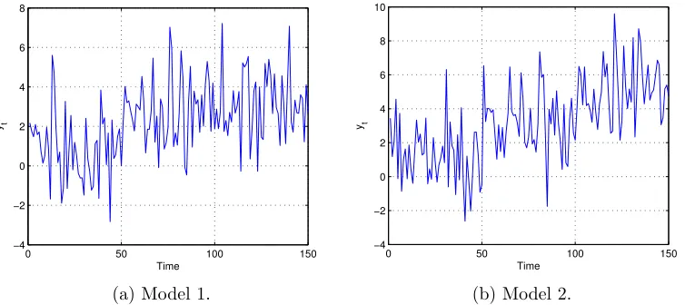
[image:11.612.118.495.109.277.2](b) Model 2.
Figure 2: Random realizations of Model 1 and Model 2.
5
A Monte Carlo Study: the Normal Mean-Shift Model
5.1
The Model
In this section, we first study the normal mean-shift model with known varianceσ2. Suppose
the normal data Yn = (y1, . . . , yn)′ is subject to unknown k changes in mean. We use the
following hierarchical model
yt|θi ∼N(θi, σ2) if τi−1 < t≤τi,
θi |µ, υ2 ∼N(µ, υ2),
(µ, υ2)∼Inv-Gamma(υ2 |a, b),
(21)
where σ2 is known and τ
i (i = 1, . . . , k) is the change-point. We set τ0 = 0 and τk+1 = n.
Next, we apply our algorithm to the case of unknown variance. In addition to (21), we
assume the Inverse-Gamma prior for σ2
σ2 ∼Inv-Gamma(σ2 |c, d). (22)
All derivations of the full conditionals and the Gibbs samplers are given in the Appendix.
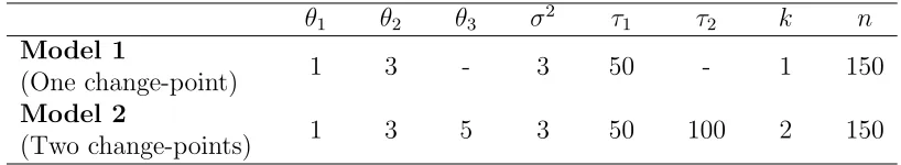
We simulate two normal sequences with the parameters specified in Table 2. Specifically,
Model 1 is subject to one change-point occurring at t = 50. Model 2 is a two change-points
model with breaks at t = 50 and t = 100. Both models assume variance σ2 = 3. Two
Table 2: Normal Mean-Shift Models 1 and 2.
θ1 θ2 θ3 σ2 τ1 τ2 k n
Model 1
1 3 - 3 50 - 1 150
(One change-point) Model 2
1 3 5 3 50 100 2 150
(Two change-points)
5.2
Simulation results
To implement our algorithm, we set the inverse-Gamma hyperparametersa=b =c=d= 1,
and the DPHMM parameters α = 3 and β = 2. The two Gibbs samplers for the cases of
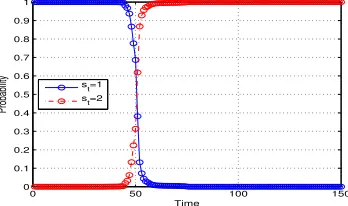
known and unknown variance are conducted for 5000 sweeps with 5000 burn-in samples, respectively. The 5000 sweeps after the burn-in period are thinned with 50 draws to reduce dependence of iterations. The first column of Figure 3 shows the probabilities of regime
indicator st =i of the two models. Intersections of the lines st =i clearly demonstrate the
break locations.
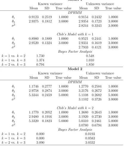
To compare our proposed DPHMM to Chib’s method, we also report the posterior infer-ence of Chib’s model under the true change-point number and the same model specification
as in (A-3) and (A-4).3 The posterior means and standard deviations of parameters are
summarized in Table 3. First, our method performs well in all cases where the posterior dis-tributions concentrate on the true values. The sample first-order serial correlations demon-strate good mixing of the samplers. Second, our results are comparable to those estimated from Chib’s model. The Bayes factors show that in most of the cases the models with the true number of change-points are preferred to others. For example, in Model 2 where two
change-points exist, the Bayes factors comparing models with k = 1 versus k = 2 are close
to zero favoring the two change-point model. Likewise, the Bayes factors comparing k = 2
versusk = 3 favor the two change-point model. Hence we conclude that the model with two
change-points is correctly specified with high probability. However, the Bayes factor fails to detect the correct number of changes in Model 1 with unknown variance. The values suggest a model with two change points. The posterior probabilities of states estimated by Chib’s model are shown in the second column of Figure 3. In summary, the simulation results demonstrate that our algorithm works well in the normal mean-shift models and is robust to the change-point number compared to Chib’s model.
3
0 50 100 150 0 0.1 0.2 0.3 0.4 0.5 0.6 0.7 0.8 0.9 1 Time Probability
st=1 st=2
DPHMM: Model 1 with known variance.
0 50 100 150
0 0.1 0.2 0.3 0.4 0.5 0.6 0.7 0.8 0.9 1 Time Probability
st=1
st=2
Chib: Model 1 with known variance.
0 50 100 150
0 0.1 0.2 0.3 0.4 0.5 0.6 0.7 0.8 0.9 1 Time Probability
st=1
st=2
DPHMM: Model 1 with unknown variance.
0 50 100 150
0 0.1 0.2 0.3 0.4 0.5 0.6 0.7 0.8 0.9 1 Time Probability
st=1
st=2
Chib: Model 1 with unknown variance.
0 50 100 150
0 0.1 0.2 0.3 0.4 0.5 0.6 0.7 0.8 0.9 1 Time Probability
st=1
st=2
st=3
DPHMM: Model 2 with known variance.
0 50 100 150
0 0.1 0.2 0.3 0.4 0.5 0.6 0.7 0.8 0.9 1 Time Probability
st=1 st=2 st=3
Chib: Model 2 with known variance.
0 50 100 150
0 0.1 0.2 0.3 0.4 0.5 0.6 0.7 0.8 0.9 1 Time Probability
st=1 st=2 st=3
DPHMM: Model 2 with unknown variance.
0 50 100 150
0 0.1 0.2 0.3 0.4 0.5 0.6 0.7 0.8 0.9 1 Time Probability
st=1 st=2 st=3
[image:13.612.117.291.122.225.2]Chib: Model 2 with unknown variance.
Table 3: Posterior estimates of Normal Mean-Shift Models 1 and 2.
Model 1
Known variance Unknown variance
Mean SD True value Mean SD True value
DPHMM
θ1 0.9123 0.2519 1.0000 0.9154 0.2432 1.0000
θ2 2.9375 0.1812 3.0000 2.9354 0.1723 3.0000
σ2 2.8244 0.3343 3.0000
Chib’s Model with k = 1
θ1 0.8980 0.1889 1.0000 0.9521 0.2441 1.0000
θ2 2.9520 0.1324 3.0000 2.9331 0.1619 3.0000
σ2 2.7933 0.4121 3.0000
Bayes Factor Analysis
k = 1 vs. k = 2 1.730 0.548
k = 1 vs. k = 3 1.374 1.010
k = 2 vs. k = 3 0.794 1.850
Model 2
Known variance Unknown variance
Mean SD True value Mean SD True value
DPHMM
θ1 1.1746 0.2777 1.0000 1.2770 0.2584 1.0000
θ2 2.9758 0.2874 3.0000 3.2176 0.2672 3.0000
θ3 5.3344 0.2459 5.0000 5.1108 0.2682 5.0000
σ2 3.1102 0.3726 3.0000
Chib’s Model with k = 2
θ1 1.1770 0.2052 1.0000 1.3680 0.2643 1.0000
θ2 2.9480 0.1916 3.0000 3.1920 0.2730 3.0000
θ3 5.3320 0.1823 5.0000 5.0310 0.2461 5.0000
σ2 3.0780 0.6794 3.0000
Bayes Factor Analysis
k = 1 vs. k = 2 0.000 0.0193
k = 1 vs. k = 3 0.000 0.0583
k = 2 vs. k = 3 3.090 3.0332
5.3
Robustness check of change-point number
In this section, we study the robustness of our algorithm in detecting the true number of change-points. Although our method does not require prespecification of the change-point number, it is still possible that our algorithm fails to estimate the correct number of change-points. Thus, we replicate the entire estimation process as in the previous section for 1000 times and record the estimated change-point number in each replication. Specifically, in each of the 1000 replications, we iterate the Gibbs sampler for 5000 times and the change-point number of the last sample is recorded. Therefore, we obtain 1000 collections of change-point numbers. Table 4 reports the frequencies of the detected change-point numbers. We see that
with high frequency (over 99%) our method detects one change-point (k = 1) in Model 1
in both cases of known and unknown variance. In Model 2, our results show that over 90%
of the 1000 replications detect two change-points (k = 2), and over 99% detect at least one
[image:15.612.110.499.347.436.2]change-point. The figures demonstrate that our algorithm correctly detects the change-point number with high probability in different cases.
Table 4: Frequencies of estimated change-point numbers.
Known variance Unknown variance
k = 0 k = 1 k = 2 k = 0 k= 1 k= 2 Model 1
0.3% 99.7% 0.0% 0.5% 99.5% 0.0%
(One change-point) Model 2
0.0% 6.5% 93.5% 0.2% 8.7% 91.1%
(Two change-points)
6
Learning
α
and
β
In the previous section, we set the DPHMM parameters α = 3 andβ = 2 in estimating the
simulated models. In order to learn aboutα andβ, we propose to use vague Gamma priors,
see Beal, Ghahramani, and Rasmussen (2002). Note that with the number of states specified in each MCMC sweep, the DPHMM reduces to the generalized Dirichlet distribution (GDD), see Connor and Mosimann (1969) and Wong (1998). Hence the posterior is
p(α, β |Sn)∝Gamma(aα, bα)Gamma(aβ, bβ) k+1 Y
i=1
βΓ(α+β) Γ(α)
Γ(nii+α)
Γ(nii+ 1 +α+β)
, (23)
where nii =PTt=1−1δ(st, i)δ(st+1, i) denotes the counts of self transitions. We set aα =bα =
aβ = bβ = 1 here and in the subsequent sections. Below we consider two alternative
6.1
The Maximum-a-Posteriori
We first solve for the maximum-a-posteriori (MAP) for α and β which are obtained as the
solutions to the following gradients using Newton-Raphson method,
∂lnp(α, β |Sn)
∂α =
aα−1
α −bα+
k+1 X
i=1
[ψ(α+β) +ψ(nii+α)−ψ(α)−ψ(nii+ 1 +α+β)] = 0
∂lnp(α, β |Sn)
∂β =
aβ−1
β −bβ +
k+1 X
i=1
1
β +ψ(α+β)−ψ(nii+ 1 +α+β)
= 0,
(24)
where ψ(·) is the digamma function defined asψ(x) =dln Γ(x)/dx.
We implement our algorithm in the previous section together with the MAP update of α
and β in each sweep. The DPHMM with MAP update correctly detects the true number of
change-points in all cases. Table 5 shows the MAP solutions for α and β, and the posterior
estimates of all parameters in each model. We can see that the average MAP values ofαand
β are 0.6353 and 0.1937 respectively in Model 1 with known and unknown variance. The
results are slightly different in Model 2 such that average MAP values are 0.9451 and 0.2360
respectively. We also report the sample standard errors which show evidence of stability of
the MAP values after the burn-in period. In all cases, α is greater than β indicating that
the algorithm tends to linger in existing states rather than exploring a new one. Besides, all
parameter estimates are in line with the results in the previous section when α and β are
prespecified.
6.2
The Metropolis-Hastings Sampler
We also consider a Metropolis-Hastings (M-H) sampler for the posterior (23). The candidate-generating density is assumed to be the random walk process with positive support
f(α′|α)∝φ(α′−α), α′ >0, (25)
whereα is the value of the previous draw,φ(·) is the standard normal density function. The
acceptance ratio, givenβ is thus
A(α, α′) = p(α
′, β |S
n) Φ(α)
p(α, β |Sn) Φ(α′)
, (26)
where Φ(·) is the standard normal distribution function. The same M-H sampler is also
applied to β given the updatedα. We incorporate the M-H sampler ofα andβ in the Gibbs
sampler in Section 5. The posterior estimators are shown in Table 6. The posterior means
and standard deviations of parameterθi andσ2 are similar to those obtained in the previous
This affirms the conclusion in the MAP results that the algorithm tends to linger in existing states rather than exploring a new one. Both the MAP and M-H methods correctly estimate the number of change-points in each simulation.
6.3
Comparison between MAP and M-H
We can see that the estimates ofαandβfrom the two approaches are quite different as shown
in Tables 5 and 6. The MAP as a point estimator may not reflect the variations of αand β,
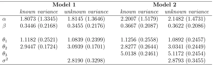
[image:17.612.73.517.315.448.2]whereas the M-H is a typical Bayesian method which can be incorporated into the MCMC sampler of other parameters in question. Moreover, the MAP approach may be limited when the posterior happens to be multi-modal. Therefore, the M-H method is preferred in practice and the following empirical studies are conducted with the M-H sampler.
Table 5: MAP of α and β in Normal Mean-Shift Models 1 and 2.
Model 1 Model 2
known variance unknown variance known variance unknown variance
α 0.6353 (0.0007) 0.6353 (0.0007) 0.9453 (0.0008) 0.9451 (0.0005)
β 0.1937 (0.0005) 0.1937 (0.0005) 0.2364 (0.0001) 0.2361 (0.0005)
θ1 0.9145 (0.2560) 0.9049 (0.2430) 1.1843 (0.2847) 1.2675 (0.2585)
θ2 2.9326 (0.1745) 2.9385 (0.1731) 2.9859 (0.2892) 3.2222 (0.2716)
θ3 5.3349 (0.2468) 5.1026 (0.2661)
σ2 2.8207 (0.3340) 3.0908 (0.3752)
Note: Average MAP values of α and β are reported with standard deviations within
parentheses. For other parameters, the values are posterior means and posterior standard deviations.
Table 6: M-H sampler of α and β in Normal Mean-Shift Models 1 and 2.
Model 1 Model 2
known variance unknown variance known variance unknown variance
α 1.8073 (1.3345) 1.8145 (1.3646) 2.2007 (1.5179) 2.1482 (1.4731)
β 0.3446 (0.2168) 0.3455 (0.2176) 0.3667 (0.2087) 0.3622 (0.2086)
θ1 1.1182 (0.2521) 1.0839 (0.2399) 1.1256 (0.2558) 1.0892 (0.2457)
θ2 2.9447 (0.1724) 3.0939 (0.1701) 2.8277 (0.2644) 3.0341 (0.2449)
θ3 5.0138 (0.2461) 5.1172 (0.2454)
σ2 2.8190 (0.3298) 2.8793 (0.3455)
[image:17.612.73.515.528.663.2]7
Empirical Applications
7.1
Poisson Data with Change-Point
We first apply our Dirichlet process multiple change-point model to the much analyzed data set on the number of coal-mining disasters by year in Britain over the period 1951–1962 (Jarrett (1979), Carlin, Gelfand, and Smith (1992) and Chib (1998)).
Let the disaster count y be modeled by a Poisson distribution
f(y |λ) =λye−λ/y!. (27)
The observation sequenceYn= (y1, y2, . . . , y112)′ is subject to some unknown change-points.
We plot the data yt in Figure 4. Chib (1998) estimates the models with one change-point
(k = 1) and with two change-points (k = 2), respectively. He assumes the parameter λ
following the prior Gamma(2,1) in the one-change-point case and the prior Gamma(3,1) in
the other. Hence, given the regime indicators Sn, the corresponding parameter λi in regime
i has the following posteriors with respect to the two priors
Posterior 1: λi |Sn, Yn∼Gamma(λi |2 +Ui,1 +Ni), (28)
and
Posterior 2: λi |Sn, Yn∼Gamma(λi |3 +Ui,1 +Ni), (29)
where Ui = P112t=1δ(st, i)yt and Ni = P112t=1δ(st, i). We perform our algorithm with the
following Gibbs steps:
Step 1. Sample Sn|λ, Yn as in (16) and obtain k,
Step 2. Sample λi |Sn, Yn as in (28) or (29),
Step 3. Update α and β with the Metropolis-Hastings Sampler as in Section 6.2.
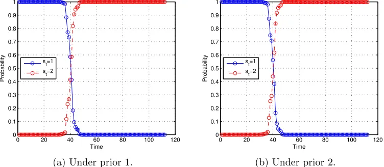
The above Gibbs sampler is conducted for 5000 sweeps with 1000 burn-in samples. To reduce the sampler dependency, the 5000 sweeps are thinned by 50 draws. The sampler estimates one change-point in the data. Figure 5 shows the posterior probabilities of the
regime indicator st =i at each time point t. The intersections of the two lines st = 1 and
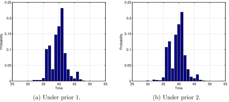
st = 2 show that the break location exits at aroundt= 40. Figure 6 provides the distribution
of the transition pointsτi. Interestingly, our model produces exactly the same figure as the
one in Chib (1998). The change-point is identified as occurring at around t = 41.
The corresponding posterior means of the parameters λ1 and λ2 are 3.1006 and 0.9387
with posterior standard deviations, 0.2833 and 0.1168, respectively, under the prior Gamma(2,1).
0 20 40 60 80 100 120 0
1 2 3 4 5 6 7
Time
[image:19.612.118.502.150.299.2]y t
Figure 4: Data on coal mining disaster count yt.
0 20 40 60 80 100 120
0 0.1 0.2 0.3 0.4 0.5 0.6 0.7 0.8 0.9 1
Time
Probability
st=1
s
t=2
(a) Under prior 1.
0 20 40 60 80 100 120
0 0.1 0.2 0.3 0.4 0.5 0.6 0.7 0.8 0.9 1
Time
Probability
st=1
s t=2
(b) Under prior 2.
[image:19.612.116.492.460.624.2]25 30 35 40 45 50 55 0
0.05 0.1 0.15 0.2 0.25
Time
Probability
(a) Under prior 1.
25 30 35 40 45 50 55
0 0.05 0.1 0.15 0.2 0.25
Time
Probability
[image:20.612.113.492.109.278.2](b) Under prior 2.
Figure 6: Posterior probability mass function of change-point location τi.
0.2464. When using the prior Gamma(3,1), we have the posterior means of λ1 and λ2 equal
to 3.1308 and 0.9567 with posterior standard deviations 0.2877 and 0.1218, respectively.
The posterior means of α and β are 1.8375 and 0.3715 with standard deviations 1.3456 and
0.2360, respectively under prior 2. All our results closely match those of the literature and
we show a certain robustness of our model under different prior assumptions.
In order to check the robustness of the estimation of the number of change-points, k,
we conduct 1000 replications of the above estimation process and collect 1000 change-point
numbers. When the first prior is assumed, 77.23% of the 1000 replications detect one
change-point. We find a similar result for prior 2. Hence, we conclude that without assuming the
number of change-points a priori, our algorithm detects the same change-point number as
in the model developed by Chib (1998) with high probability.
7.2
Real Output
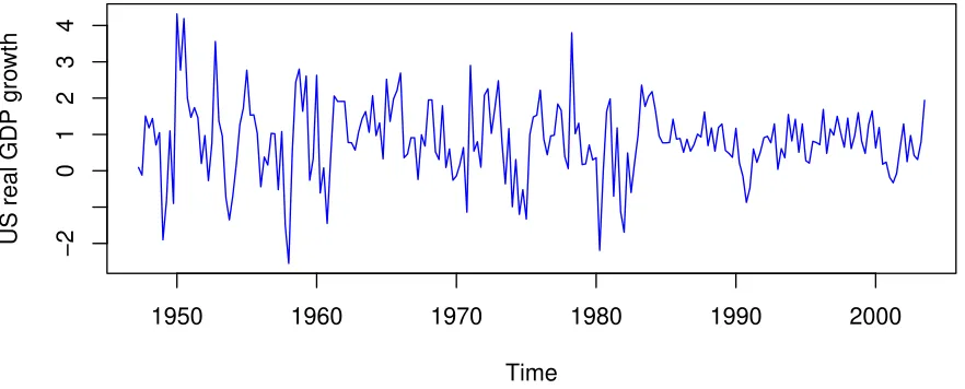
We also apply our algorithm to estimate structural changes in real GDP growth. The data and model are drawn from Maheu and Gordon (2008) (see also Geweke and Yu (2011)). Let
yt= 100[log(qt/qt−1)−log(pt/pt−1)], whereqtis quarterly US GDP seasonally adjusted andpt
is the GDP price index. The data range from the second quarter of 1947 to the third quarter of 2003, for a total of 226 observations (see Figure 7). We model the data with a Bayesian
ar(2) model with structural change. The frequentist autoregressive structural change-model
can be found in Chong (2001). Suppose the data are subject to k change-points and follow
yt=β0,st +β1,styt−1+β2,styt−2+εt, εt∼N(0, σ
2
st), st= 1,2, . . . , k + 1. (30) We assume the following hierarchical priors to β0,i, β1,i and β2,i
Time
US real GDP gro
wth
1950 1960 1970 1980 1990 2000
−2
0
1
2
3
[image:21.612.76.517.142.320.2]4
Figure 7: US real GDP growth from the second quarter of 1947 to the third quarter of 2003.
where µ= (µ0, µ1, µ2)′ and V = Diag(v20, v21, v22), such that
p(µj, v2j)∝Inv-Gamma(vj2 |a, b), j = 0,1,2. (32)
We assume the noninformative prior for σ2
i such that
p(σ2i)∝1/σ2i, i= 1, . . . , k+ 1. (33)
Conditional on σ2
i, the sampling of βi, µ and V is similar to Section 5. For σ2i, we can
draw from the following full conditional
σ2
i |βi, Sn, Yn∼Inv-χ2
σ2
i |τi−τi−1,
ω2
i
τi−τi−1
, i= 1, . . . , k+ 1, (34)
where ω2
i =
P
τi−1<t≤τi(yt−β0,st −β1,styt−1−β2,styt−2)
2.
As in the previous applications, we set the inverse-Gamma hyperparameters a =b = 1.
The M-H update of α and β follows the discussion in Section 6.2. The Gibbs sampler is
conducted for 5000 sweeps with 1000 burn-in samples. The 5000 sweeps are thinned by
50 draws. The posterior probabilities of the regime indicator st in Figure 8a suggest that
the structural break exists between the years 1980 and 1990. Figure 8b further shows the change-point at the second quarter of 1983, which is close to the results in Maheu and Gordon
(2008).4 The posterior estimates are summarized in Table 7. Finally, the posterior means of
α and β are 1.7749 and 0.3045 with standard deviations 1.3422 and 0.1939 respectively. All
of our results are consistent with Chib’s estimates. 4
19400 1950 1960 1970 1980 1990 2000 2010 0.1
0.2 0.3 0.4 0.5 0.6 0.7 0.8 0.9 1
Time
Probability
st=1
st=2
(a) Posterior probability ofst=i.
1981:10 1982:1 1983:2 1984:3 1985:4 1986:4
0.05 0.1 0.15 0.2 0.25 0.3 0.35
Time
Probability
[image:22.612.116.493.172.340.2](b) Posterior probability of break locationτi.
Figure 8: US real GDP growth structural change model.
Table 7: US real GDP growth structural change model with one change-point.
Chib’s Model DPHMM
st= 1 st= 2 st= 1 st= 2
β0,st 0.5642 (0.1228) 0.4434 (0.1162) 0.5499 (0.1303) 0.3894 (0.1169)
β1,st 0.2716 (0.0734) 0.2792 (0.1052) 0.2812 (0.0837) 0.2796 (0.1173)
β2,st 0.0800 (0.0739) 0.1588 (0.1010) 0.0913 (0.0855) 0.2253 (0.1124)
σ2
st 1.3331 (0.1542) 0.3362 (0.0516) 1.4089 (0.1722) 0.2672 (0.0460)
Note:
[image:22.612.73.503.524.613.2]Finally, we replicate 1000 times the whole estimation process and check the robustness of the detected change-point number. The result suggests that nearly 100% of the replications detect one break point.
8
Concluding Remarks
In this paper, we have proposed a new Bayesian multiple change-point model, that is the Dirichlet process hidden Markov model. Our model is semiparametric in the sense that the number of states is not built-in to the model but endogenously determined. As a result, our model avoids the model misspecification problem. We have proposed an MCMC sampler which only needs to sample the states around change-points. We have also proposed the MAP and M-H updates of hyperparameters in the DPHMM process. We have presented three specific models, namely, the discrete Poisson model, the continuous normal model,
and the ar(2) model with structural changes. Results from the simulations and empirical
Appendix
In the appendix, we give the derivations of the full conditionals and the Gibbs samplers in Section 5. For the case of known variance, we first rewrite the hierarchical model (21) as the joint distribution
p(Yn, θ, µ, υ2 |Sn, σ2)∝ k+1 Y
i=1
N(˜yi |θi, σ2i) k+1 Y
i=1
N(θi |µ, υ2)p(µ, υ2), (A-1)
where p(µ, υ2) corresponds to Inv-Gamma(υ2 |a, b), θ= (θ
1, . . . , θk+1)′ and
˜
yi =
P
τi−1<t≤τiyt
τi−τi−1
, and σ2i = σ
2
τi−τi−1
. (A-2)
From (A-1) and (A-2), we have the following full conditionals
p(θi |µ, υ2, σ2, Sn, Yn)∝ k+1 Y
i=1
N(˜yi |θi, σi2)N(θi |µ, υ2)
∝N
θi |
˜
yi/σi2+µ/υ2
1/σ2
i + 1/υ2
, 1
1/σ2
i + 1/υ2
,
p(µ|θ, υ2, Sn, Yn)∝ k+1 Y
i=1
N(θi |µ, υ2)p(µ, υ2)
∝N(µ|θ, υ¯ 2/(k+ 1)),
p(υ2 |θ, µ, Sn, Yn)∝(υ2)−(k+1)/2exp
( −1 2 k+1 X i=1
(θi−µ)2/υ2
)
p(µ, υ2)
∝Inv-Gamma υ2 |a+ k+ 1
2 , b+
1 2
k+1 X
i=1
(θi−µ)2
!
,
(A-3)
where ¯θ=Pk+1
i=1 θi/(k+ 1). Therefore, we can perform the following Gibbs sampler
Step 1. Sample Sn|θ, µ, υ, Yn as in (16) and obtaink,
Step 2. Sample θ, µ, υ |Sn, Yn as in (A-3).
For the case of unknown variance, the full conditional with respect to (22) is
σ2 |θ, Sn, Yn ∼Inv-Gamma σ2
c+ n 2, d+
1 2
n
X
t=1
(yt−θst)
2 !
. (A-4)
Conditional on σ2, we apply the same estimation strategy discussed above. The Gibbs
Step 1. Sample Sn|θ, µ, υ, σ2, Yn as in (16) and obtain k,
Step 2. Sample θ, µ, υ, σ2 |S
References
Beal, M. J., Z. Ghahramani, and C. E. Rasmussen (2002): “The Infinite Hidden
Markov Model,” in Advances in Neural Information Processing Systems, ed. by T. G.
Dietterich, S. Becker, and Z. Ghahramani, Advances in Neural Information Processing
Systems, pp. 577–584. MIT Press.
Blackwell, D., and J. B. MacQueen (1973): “Ferguson Distributions Via Polya Urn
Schemes,”The Annals of Statistics, 1(2), 353–355.
Carlin, P. B., A. E. Gelfand, and A. F. M. Smith (1992): “Hierarchical Bayesian
Analysis of Changepoint Problems,” Journal of the Royal Statistical Society. Series C
(Applied Statistics), 41(2), 389–405.
Chernoff, H., and S. Zacks (1964): “Estimating the Current Mean of a Normal
Distri-bution which is Subjected to Changes in Time,” The Annals of Mathematical Statistics,
35(3), pp. 999–1018.
Chib, S.(1998): “Estimation and comparison of multiple change-point models,” Journal of
Econometrics, 86(2), 221 – 241.
Chong, T. T.-L. (2001): “Structural Change in AR(1) Models,” Econometric Theory, 17(1), 87–155.
Connor, R. J., and J. E. Mosimann(1969): “Concepts of Independence for Proportions
with a Generalization of the Dirichlet Distribution,” Journal of the American Statistical
Association, 64(325), pp. 194–206.
Ferguson, T. S. (1973): “A Bayesian analysis of some nonparametric problems,” Annals
of Statistics, 1, 209–230.
Geweke, J., and J. Yu (2011): “Inference and prediction in a multiple-structural-break
model,”Journal of Econometrics, In Press.
Giordani, P., and R. Kohn (2008): “Efficient Bayesian Inference for Multiple
Change-Point and Mixture Innovation Models,” Journal of Business and Economic Statistics,
26(1), 66–77.
Jarrett, R. G. (1979): “A Note on the Intervals Between Coal-Mining Disasters,”
Biometrika, 66(1), 191–193.
Koop, G., and S. M. Potter (2007): “Estimation and Forecasting in Models with
Mul-tiple Breaks,”The Review of Economic Studies, 74(3), pp. 763–789.
Kozumi, H., and H. Hasegawa (2000): “A Bayesian analysis of structural changes with
Maheu, J. M., and S. Gordon (2008): “Learning, forecasting and structural breaks,”
Journal of Applied Econometrics, 23(5), 553–583.
Neal, R. M.(1992): “The Infinite Hidden Markov Model,” inProceedings of the Workshop
on Maximum Entropy and Bayesian Methods of Statistical Analysis, ed. by C. R. Smith,
G. J. Erickson,and P. O. Neudorfer, Proceedings of the Workshop on Maximum Entropy
and Bayesian Methods of Statistical Analysis, pp. 197–211. Kluwer Academic Publishers.
(2000): “Markov Sampling Methods for Dirichlet Process Mixture Models,”Journal
of Computational and Graphical Statistics, 9(2), 249–265.
Pesaran, M. H., D. Pettenuzzo, and A. Timmermann (2006): “Forecasting Time
Series Subject to Multiple Structural Breaks,”Review of Economic Studies, 73(4), 1057–
1084.
Sethuraman, J.(1994): “A Constructive Definition of Dirichlet Priors,” Statistica Sinica, 4(2), 639–650.
Smith, A. F. M. (1975): “A Bayesian approach to inference about a change-point in a
sequence of random variables,”Biometrika, 62, 407–416.
Stephens, D. A. (1994): “Bayesian Retrospective Multiple-Changepoint Identification,”
Journal of the Royal Statistical Society. Series C (Applied Statistics), 43(1), 159–178.
Wang, J., and E. Zivot (2000): “A Bayesian Time Series Model of Multiple Structural
Changes in Level, Trend, and Variance,”Journal of Business & Economic Statistics, 18(3),
374–386.
Wong, T.(1998): “Generalized Dirichlet distribution in Bayesian analysis,” Applied