Asynchronous Adaptation and Learning Over Networks—Part II: Performance Analysis

arXiv:1312.5438v3 [cs.SY] 16 Dec 2014

Asynchronous Adaptation and Learning over

Networks — Part II: Performance Analysis

Xiaochuan Zhao, Student Member, IEEE, and Ali H. Sayed, Fellow, IEEE

Abstract

In Part I [2], we introduced a fairly general model for asynchronous events over adaptive networks including random topologies, random link failures, random data arrival times, and agents turning on and off randomly. We performed a stability analysis and established the notable fact that the network is still able to converge in the mean-square-error sense to the desired solution. Once stable behavior is guaranteed, it becomes important to evaluate how fast the iterates converge and how close they get to the optimal solution. This is a demanding task due to the various asynchronous events and due to the fact that agents influence each other. In this Part II, we carry out a detailed analysis of the mean-square-error performance of asynchronous strategies for solving distributed optimization and adaptation problems over networks. We derive analytical expressions for the mean-square convergence rate and the steady-state mean-square-deviation. The expressions reveal how the various parameters of the asynchronous behavior influence network performance. In the process, we establish the interesting conclusion that even under the influence of asynchronous events, all agents in the adaptive network can still reach an O(ν1+γ′

o) near-agreement with someγ′

o>0while approaching the desired solution withinO(ν) accuracy, where

ν is proportional to the small step-size parameter for adaptation.

Index Terms

Distributed learning, distributed optimization, diffusion adaptation, asynchronous behavior, adaptive networks, dynamic topology, link failures.

The authors are with Department of Electrical Engineering, University of California, Los Angeles, CA 90095 Email:

{xzhao, sayed}@ee.ucla.edu.

This work was supported by NSF grants CCF-1011918 and ECCS-1407712. A short and limited early version of this work appeared in the conference proceeding [1]. The first part of this work is presented in [2].

I. INTRODUCTION

In Part I [2], we introduced a fairly general model for asynchronous distributed adaptation and learning over networks. The model allows the step-size for any agent to be randomly chosen within a range of values including zero, meaning an off-status; it also allows the communication links between any two agents to be randomly turned on and off; it further allows the topology to vary and the combination weights on the links between agents to vary randomly. The model also captures the situation in which agents randomly select a subset of their neighbors to share information with, as happens in gossip implementations. Based on this asynchronous model, we carried out a detailed stability analysis in Part I [2] and arrived at Theorem 1 in that Part, which provides an explicit condition on the first and second-order moments of the distribution of the step-sizes to ensure mean-square stability of the adaptive network. When the condition holds, it was further shown that the asymptotic mean-square-deviation (MSD) for every agent in the network remains bounded. Interestingly, it was shown that these conclusions hold irrespective of the randomness in the network topology.

In this Part II, we conduct a detailed mean-square-error (MSE) analysis in order to characterize the learning behavior of the asynchronous network in terms of the network parameters. In particular, we answer the following three questions:

• How is the convergence rate of the algorithm affected by the occurrence of asynchronous events in comparison to a synchronous network?

• Are agents still able to reach some sort of agreement in steady-state despite the various sources of randomness influencing their interactions?

• How close do the iterates of the various agents get to each other and to the desired optimal solution? One of the main conclusions that will follow from the analysis is that, under certain reasonable conditions, the asynchronous network will continue to be able to deliver performance that is comparable to the synchronous case where no failures occur. In particular, we will be able to establish that for a sufficiently small step-size parameterν it holds that

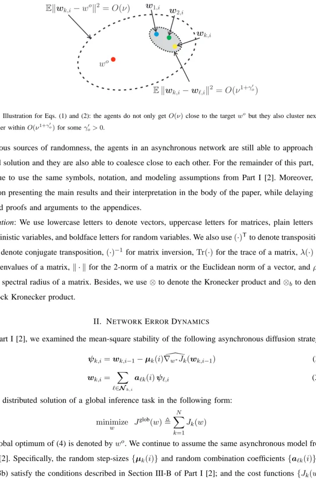
lim i→∞ E_kwo_−w k,ik2 =O(ν) (1) lim i→∞ E_{kwk,i−wℓ,ik}2 _=O(ν1+γ′ o) ₍₂₎

for someγ_o′ >0 that is given by (92) further ahead. These results imply that all agents reach a level of

O(ν1+γ′

o) agreement with each other and getO(ν) close to the desired optimal solution,wo, in

Fig. 1. Illustration for Eqs. (1) and (2): the agents do not only get O(ν)close to the targetwo

but they also cluster next to each other withinO(ν1+γ′

o)_{for someγo}′ _>0_.

to various sources of randomness, the agents in an asynchronous network are still able to approach the desired solution and they are also able to coalesce close to each other. For the remainder of this part, we continue to use the same symbols, notation, and modeling assumptions from Part I [2]. Moreover, we focus on presenting the main results and their interpretation in the body of the paper, while delaying the detailed proofs and arguments to the appendices.

Notation: We use lowercase letters to denote vectors, uppercase letters for matrices, plain letters for

deterministic variables, and boldface letters for random variables. We also use(_·)T_{to denote transposition,}

(_·)∗ to denote conjugate transposition,(_·)−1 for matrix inversion,Tr(_·) for the trace of a matrix,λ(_·) for the eigenvalues of a matrix, _{k · k} for the 2-norm of a matrix or the Euclidean norm of a vector, andρ(_·)

for the spectral radius of a matrix. Besides, we use⊗to denote the Kronecker product and⊗b to denote

the block Kronecker product.

II. NETWORKERRORDYNAMICS

In Part I [2], we examined the mean-square stability of the following asynchronous diffusion strategy:

ψ_k,i=w_k,i−1−µk(i)∇\w∗J_k(w_k,i−1) (3a)

wk,i=

X

ℓ∈Nk,i

aℓk(i)ψℓ,i (3b)

for the distributed solution of a global inference task in the following form:

minimize w J glob_(w), N X k=1 Jk(w) (4)

The global optimum of (4) is denoted bywo. We continue to assume the same asynchronous model from Part I [2]. Specifically, the random step-sizes _{µk(i)} and random combination coefficients{aℓk(i)} in

satisfy Assumptions 1 and 2 in Section II of Part I [2]. However, in order to study the mean-square-error performance in steady-state, it is necessary to strengthen the assumption on the stochastic gradient vectors

{∇\w∗J_k(w_k,i−1)}. We replace the gradient noise model described in Assumption 3 in Section III-A of

Part I [2] by the following one.

Assumption 1 (Gradient noise model):

1) The gradient noise v_k,i(w_k,i−1), conditioned on Fi−1, is assumed to be independent of any other

random sources including topology, links, combination coefficients, and step-sizes. The conditional moments ofv_k,i(w_k,i−1) satisfy:

E_{[vk,i(wk,i−1)|}F_{i−1] = 0 (5)} E_{[kvk,i(wk,i−1)k}4_|F_i−1]≤α2_kwo_−wk,i−1k4_+σ4

v (6)

for someα_≥0 andσ_v2 _≥0.

2) The individual gradient noises _{vk,i(wk,i−1)} are uncorrelated and circular across all agents such

that

Ri(wi−1) = diag{R1,i(w1,i−1), . . . , RN,i(wN,i−1)} (7)

where _Ri(wi−1) and {Rk,i(wk,i−1)} are from (23) and (19) both in Part I [2].

3) The conditional covariance of

¯

vi(wi−1) satisfies the Lipschitz condition

kRi(1N ⊗wo)− Ri(wi−1)k ≤κvk1N ⊗wo−wi−1kγv (8)

for some constantsκv ≥0 and0< γv ≤4.

4) The covariance of

¯

v_i(1N⊗wo) converges to a constant matrix: R, lim i→∞Ri(1N⊗w o_),diag {R1, . . . , RN} (9) where Rk , lim i→∞Rk,i(w o_{) (10)}

From Assumption 1, the conditional moments of

¯

vk,i(wk,i−1) satisfy E_[ ¯vk,i(wk,i−1)|Fi−1] = 0 (11) E_[k ¯ v_k,i(w_k,i−1)k4|Fi−1]≤α2k ¯ wo₋ ¯ w_k,i−1k4+ 4σ4v (12)

where a factor of 4 appeared due to the transform

¯

A. Long Term Error Dynamics

We showed in (87) from Part I [2] that the error recursion for the asynchronous network (3a)–(3b) evolves according to the following dynamics:

¯e wi =ATi (I2M N −MiHi−1) ¯e wi−1+ATi Mi ¯ vi(wi−1) (13)

where H_i−1 = diag_{H1,i−1,H2,i−1, . . . ,HN,i−1} and

Hk,i−1, Z 1 0 ∇ 2 ¯ w ¯ w∗Jk( ¯ wo₋t ¯e wk,i−1)dt (14)

The dependency of H_i−1 on the previous iterate wi−1 complicates the mean-square analysis. Recall

though from Lemma 1 in Part I [2] that the Hessian matrices of the costs_{Jk( ¯

w)_} are globally Lipschitz around ¯ wo. Let Hk,∇2 ¯ w ¯ w∗J_k( ¯ wo), _H,diag_{H1, . . . , HN} (15)

Recursion (13) can then be rewritten as

¯e wi =ATi (I2M N −MiH) ¯e wi−1+ATiMi ¯ vi(wi−1) +ATidi (16)

where the perturbation factor di is given by

di,Mi(H −Hi−1) ¯e wi−1 ,col{d1,i, . . . ,dN,i} (17) dk,i,µk(i)(Hk−Hk,i−1) ¯e wk,i−1 (18)

Let µ¯(_kn) , E_[µk(i)]n _{denote the n-th moment of the random step-size parameter µ}

k(i); we also use ¯

µk ≡µ¯(1)_k from (34) of Part I [2] for the mean and cµ,k,ℓ =E[(µk(i)−µ¯k)(µℓ(i)−µ¯ℓ)] from (37) of

Part I [2] for the cross-covariance.

Lemma 1 (Size of perturbation): If condition (103) in Part I [2], namely, q ¯ µ(4)_k ¯ µ(1)_k < λk,min 3λ2 k,max+ 4α (19) holds for all k, then

lim sup i→∞ E_kAT idik2 ≤O(ν4) (20) where ν,max k q ¯ µ(4)_k ¯ µ(1)_k (21)

Assumption 2 (Small step-sizes): The parameterν from (21) is sufficiently small such that ν <min k λk,min 3λ2 k,max+ 4α <1 (22)

Under Assumption 2, condition (19) holds. It was shown in (200) and (201) from Part I [2] that condition (19) in this Part implies condition (93) from Part I [2], i.e.,

¯ µ(2)_k ¯ µ(1)_k < λk,min α+λ2_k,max (23) for all k.

Since we are interested in examining the asymptotic performance of the asynchronous network, result (20) indicates that the network error recursion (13) can be expressed for large enough i by using the following long-term model:

¯e w_i′ =AT_i(I2M N−MiH) ¯e w_i′₋₁+AT_iM_i ¯ v_i(w_i−1) (24)

where we ignore the O(ν2) term AT

idi according to (20), and we use w′i−1 to denote the estimate

obtained from this long-term model. It is worth noting that the gradient noise

¯

vi(wi−1) in (24) is an

extraneous noise that is imported from the original model (13); it only depends on the original estimate wi−1 but not on w′i−1. We will now use recursion (24) to determine expressions (rather than bounds)

for the steady-state individual MSD and for the average network MSD. One advantage of model (24) is that the random matrix H_i−1 from (13) has been replaced by the constant matrix _H. More formally, under Assumption 1 on the fourth-order moment of the gradient noise, and by extending the arguments of Appendices D and E from Part I [2] and the arguments of [3], we will establish later in (76) that the MSD expression resulting from (24) is withinO(ν3/2) of the MSD expression for the original recursion (13); this conclusion will rely on the following useful result.

Theorem 1 (Bounded mean-square gap): Under Assumptions 1 and 2, the mean-square gap from the

original error recursion (13) to the long-term model (24) is then asymptotically bounded by

lim sup i→∞ max k E_k ¯e wk,i− ¯e w′_k,ik2 ≤O(ν2) (25) for anyk.

Proof: See Appendix B.

To proceed with the mean-square-error performance analysis, we introduce the following auxiliary variables:

D_{i ,}I2M N−MiH= diag{Dk,i} (27) B_{i ,}AT_iD_i (28) ¯si ,A T iMi ¯ vi(wi−1) (29)

Based on the gradient noise model in Assumption 1 and the asynchronous network model described in Section III-B of Part I [2], it is easy to verify that the (conditional) means of_{A_i,M_i,D_k,i,D_i,B_i,

¯

s_i} are given by:

¯ A,E₍A_i) = ¯A_⊗I2M (30) ¯ M,E₍M_i) = ¯M_⊗I2M (31) ¯ Dk,E(Dk,i) =I2M −µ¯kHk (32) ¯ D,E₍D_i) =I2M N−MH¯ = diag{D¯k} (33) ¯ B,E₍B_i) = ¯_AT_D¯ (34) ¯ s_,E₍ ¯si|Fi−1) = 0 (35)

It can be verified that the block-Kronecker-covariance matrices of several random quantities are given by:

CA,E[(Ai−A¯)⊗b(Ai−A¯)] =CA⊗I4M2 (36) CM ,E[(Mi−M¯)⊗b(Mi−M¯)] =CM ⊗I4M2 (37) CD ,E[(D∗i −D¯∗)T⊗b(Di−D¯)] =CM(HT⊗bH) (38) CB,E[(B∗i −B¯∗)T⊗b(Bi−B¯)] = ( ¯AT⊗bA¯T)CD+CAT( ¯DT⊗bD¯+CD) (39)

where the symbol_⊗b denotes the block-Kronecker operation of block size2M×2M (see Appendix C).

Moreover, it can be verified by using property (133) from Appendix C that

E_[(X∗_−X¯∗)T_⊗

b(X −X¯)] =E[(X∗)T⊗bX]−( ¯X∗)T⊗bX¯ (40)

for any random block matrix X with appropriate block size and with mean _X¯ _, EX. The _{CA, CM}

that appear in (36)–(39) relate to the second-order moments of {aℓk(i)} and {µk(i)}. Using (28) and

(29), the long-term model (24) can be rewritten as

¯e

w_i′ =B_i·

¯e

w_i′₋₁+

B. Mean Error Recursion

Taking the expectation of both sides of (41), we end up with the mean error recursion for large i:

E

¯e

w_i′ = ¯_{B ·}E

¯e

w′_i−1 (42)

The stability of recursion (42) requires the stability of _B¯. A condition on the step-sizes to ensure the stability of _B¯ can be derived as follows. Using the fact that _A¯is block left-stochastic and _D¯ is block diagonal and Hermitian, and following the same argument in [4, App. A] [5], we obtain

ρ( ¯_B)_≤ρ( ¯_D) (43) whereρ(_·)denotes the spectral radius of its matrix argument. It follows from (33) and (43) that asymptotic mean stability is guaranteed if the mean step-size µ¯k satisfies

¯

µk≡µ¯(1)_k < 2

ρ(Hk)

(44) for all k. Since Hk is a positive semi-definite matrix, its spectral radius coincides with its largest

eigenvalue. Using (8) from Part I [2], we have ρ(Hk) ≤ λk,max. If condition (19) holds, then from

(196) of Part I [2], we have ¯ µ(1)_{k ≤} q ¯ µ(4)_k ¯ µ(1)_k < λk,min 3λ2_k,max+ 4α ≤ λk,min 3λ2_k,max ≤ 2 ρ(Hk) (45) since α >0. Therefore, condition (44) holds if condition (19) does so. With Assumption 2, we have

lim i→∞

E_we′

k,i= 0 (46)

for allk. From (46), we conclude that the long-term model (24) or, equivalently, (41), is the asymptotically centered version of the original error recursion (13).

C. Error Covariance Recursion

We proceed to examine the evolution of the covariance matrix of the network error vector

¯e

w_i′ in the long-term model (41). Let

ri(wi−1),bvec(Ri(wi−1)) =E[( ¯ v∗_i(wi−1))T⊗b ¯ vi(wi−1)|Fi−1] (47) yi ,( ¯AT⊗bA¯T+CAT)( ¯M ⊗bM¯ +CM)E[ri(wi−1)] (48) zi ,bvec(E( ¯e w_i′ ¯e w_i′∗)) =E_[( ¯e w′∗_i )T_⊗b ¯e w′_i] (49) G,E_[(D∗_i)T_⊗ bDi] = ¯DT⊗bD¯+CD (50)

F ,E_[(B∗_i)T_⊗bBi]∗= ¯BT⊗bB¯∗+C∗B=G( ¯A ⊗bA¯+CA) (51)

where the notationsbvec(_·)and_⊗bdenote block vectorization and block Kronecker products, respectively,

both of size2M_×2M (see Appendix C). We note that the second equalities in (47) and (49) are due to property (130) and the second equalities in (50) and (51) are by using (33), (34), and (38)–(40). Using (47)–(51), we obtain the following recursion for the block-vectorized covariance matrix of the network error vector

¯e

w′_i.

Theorem 2 (Network error covariance recursion): The vector zi evolves according to the following

recursion:

zi =F∗zi−1+yi (52)

Recursion (52) converges if condition (19) holds, and its convergence rate is determined byρ(_F).

Proof: See Appendix D.

The vectorzi can be used to compute useful error metrics. For example, we can examine any weighted

MSE measure for

¯e

w′_i by evaluating quantities of the form:

E_k ¯e w′_ik2_Σ =E_[Tr( ¯e w_i′ ¯e w′∗_i Σ)] =z_i∗_·bvec(Σ) (53) where Σ is an arbitrary positive semi-definite weight matrix. To guarantee the convergence ofE_k

¯e

w′_ik2_Σ for any weighting matrixΣ, it is sufficient and necessary to guarantee the convergence of zi. It follows

from Theorem 2 that under Assumption 2, the spectral radius of the matrix _F in (52) determines the mean-square stability and convergence rate of the asynchronous diffusion strategy (3a)–(3b).

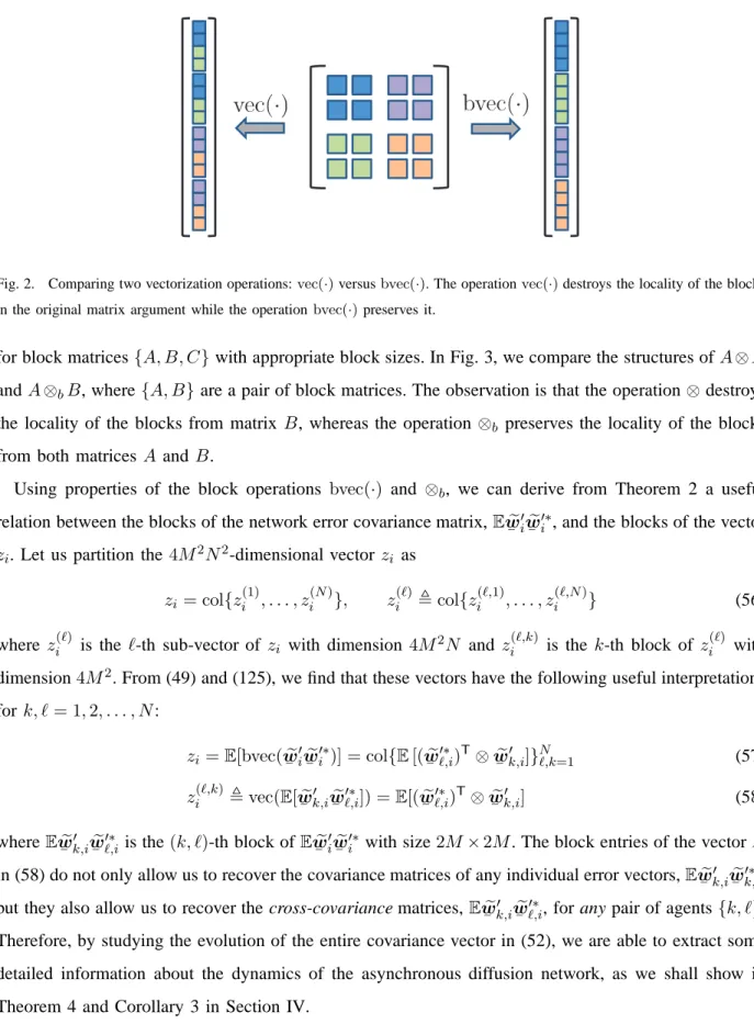
Before proceeding we comment on the reason why we choose to use the block vectorization operation

bvec(_·) in (49) instead of the traditional vectorization operationvec(_·). This is becausebvec(_·) allows us to track each block of its matrix argument after vectorization. By the definition in (125) and the illustration in Fig. 2, operationbvec(_·) preserves the locality of every block in the original matrix argument whereas operation vec(_·) blends different blocks together. Therefore, whenever we need to vectorize a network matrix whose blocks relate to individual agents, it is more natural to use the block vectorization operation

bvec(_·); on the other hand, whenever we need to vectorize a matrix that only relates to a single agent, we can use the conventional vectorization operationvec(_·). A useful property of the conventional vectorization operation vec(_·) is

vec(ABC) = (CT_⊗A)_·vec(B) (54) for matrices_{A, B, C_} of compatible sizes. A similar property holds for the bvec(_·) operation:

Fig. 2. Comparing two vectorization operations:vec(·)versusbvec(·). The operationvec(·)destroys the locality of the blocks in the original matrix argument while the operationbvec(·)preserves it.

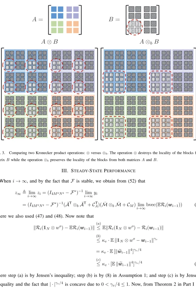
for block matrices_{A, B, C_}with appropriate block sizes. In Fig. 3, we compare the structures ofA_⊗B

andA_⊗bB, where{A, B}are a pair of block matrices. The observation is that the operation ⊗destroys

the locality of the blocks from matrix B, whereas the operation _⊗b preserves the locality of the blocks

from both matrices A and B.

Using properties of the block operations bvec(_·) and _⊗b, we can derive from Theorem 2 a useful

relation between the blocks of the network error covariance matrix,E

¯e

w′_i

¯e

w′∗_i , and the blocks of the vector

zi. Let us partition the4M2N2-dimensional vectorzi as

zi = col{z(1)i , . . . , z (N) i }, z (ℓ) i ,col{z (ℓ,1) i , . . . , z (ℓ,N) i } (56)

where z_i(ℓ) is the ℓ-th sub-vector of zi with dimension 4M2N and z(iℓ,k) is the k-th block of z

(ℓ)

i with

dimension4M2_{. From (49) and (125), we find that these vectors have the following useful interpretations}

for k, ℓ= 1,2, . . . , N: zi =E[bvec( ¯e w_i′ ¯e w′∗_i )] = col_{E_[( ¯e w′∗_ℓ,i)T_⊗ ¯e w_k,i′ ]_}N_ℓ,k=1 (57) z_i(ℓ,k),vec(E_[ ¯e w′_k,i ¯e w′∗_ℓ,i]) =E_[( ¯e w′∗_ℓ,i)T_⊗ ¯e w′_k,i] (58) whereE ¯e w′_k,i ¯e

w′∗_ℓ,i is the(k, ℓ)-th block ofE

¯e

w_i′

¯e

w′∗_i with size2M_×2M. The block entries of the vectorzi

in (58) do not only allow us to recover the covariance matrices of any individual error vectors,E

¯e

w_k,i′

¯e

w_k,i′∗, but they also allow us to recover the cross-covariance matrices,E

¯e

w_k,i′

¯e

w_ℓ,i′∗, for any pair of agents_{k, ℓ_}. Therefore, by studying the evolution of the entire covariance vector in (52), we are able to extract some detailed information about the dynamics of the asynchronous diffusion network, as we shall show in Theorem 4 and Corollary 3 in Section IV.

Fig. 3. Comparing two Kronecker product operations:⊗versus⊗b. The operation⊗destroys the locality of the blocks from matrixB while the operation⊗bpreserves the locality of the blocks from both matricesAandB.

III. STEADY-STATE PERFORMANCE

When i_{→ ∞}, and by the fact that _F is stable, we obtain from (52) that

z∞, lim i→∞zi= (I4M2N2− F ∗₎−1 _lim i→∞yi = (I4M2_N2− F∗)−1( ¯AT⊗_bA¯T+C_AT)( ¯M ⊗_bM¯ +C_M) lim i→∞bvec( E_{Ri(wi−1)) (59)}

where we also used (47) and (48). Now note that

kRi(1N ⊗wo)−ERi(wi−1)k (a) ≤ E_{kRi(1N ⊗w}o_{)− Ri(wi−1)k} (b) ≤ κv·Ek1N ⊗wo−wi−1kγv =κv·E[kwei−1k4]γv/4 (c) ≤ κv·[Ekwei−1k4]γv/4 (60)

where step (a) is by Jensen’s inequality; step (b) is by (8) in Assumption 1; and step (c) is by Jensen’s inequality and the fact that_{| · |}γv/4 _{is concave due to0< γ}

we know thatlim sup_i→∞E_kwei−1k4 _≤O(ν2_{)under Assumption 2. Therefore, we obtain from (60) that}

lim sup i→∞ kRi

(1N ⊗wo)−ERi(wi−1)k ≤O(νγv/2) (61)

According to (61), we can replace E_{Ri(wi−1) in (59) by Ri(1N ⊗w}o_{) with an error in the order of}

νγv/2_{. Let}

z,(I4M2_N2− F∗)−1( ¯AT⊗_bA¯T+C_AT)( ¯M ⊗_bM¯ +C_M)bvec(R) (62)

From (198) in Part I [2], we know that the second-order moments of _{µk(i)} are in the order of ν2.

Hence, by (84) from Part I [2], (31), and (37), it is easy to verify that

kM ⊗¯ bM¯ +CMk=O(ν2) (63)

Using (62), (63), and the fact that _k(I4M2_N2 − F∗)−1k = O(ν−1) from Lemma 5 further ahead, we

conclude that

kz_k=O(ν) (64)

Then, by using (9) and (61)–(64), we obtain from (59) that

z∞=z+O(ν1+γv/2), kz∞k=O(ν) (65)

Define the steady-state average network MSD by MSDnet , lim i→∞ 1 N N X k=1 E_kwek,ik2 ₍₆₆₎

and the steady-state individual MSD for agentk by

MSDk, lim

i→∞

E_kwek,ik2 ₍₆₇₎

Theorem 3 (Steady-state MSD): It holds that

MSDnet = 1 2Nz ∗_bvec(I 2M N) +O(ν1+γo) (68) MSDk= 1 2z ∗_bvec(E kk⊗I2M) +O(ν1+γo) (69) where z is given by (62), γo , 1 2min{1, γv} (70)

and Ekk is the N ×N basis matrix that only has one non-zero element, which is equal to 1, at the (k, k)-th entry.

Proof: From (53) by selecting Σ =I2M N, and also using (59) and (65), we get lim i→∞ E_k ¯e w_i′_k2=z_∞∗ bvec(I2M N) =z∗bvec(I2M N) +O(ν1+γv/2) =O(ν) (71)

Likewise, by selecting Σ =Ekk⊗I2M, we get lim i→∞ E_k ¯e w_i′_k2_Ekk⊗I 2M =z ∗ ∞bvec(Ekk⊗I2M) =z∗bvec(Ekk⊗I2M) +O(ν1+γv/2) =O(ν) (72)

Note further that

E_k ¯e w_ik2 =E_k ¯e w_i′_k2+E_k ¯e w_i− ¯e w_i′_k2+ 2ReE_[ ¯e w′∗_i ( ¯e w_i− ¯e w′_i)] (73)

Using the Cauchy-Schwartz inequality, it can be verified that

ReE_[ ¯e w_i′∗( ¯e wi− ¯e w_i′)]_≤ q E_k ¯e w_i′_k2_·E_k ¯e wi− ¯e w_i′_k2 (74)

From Theorem 1, we have

lim i→∞ E_k ¯e wi− ¯e w′_ik2 _≤O(ν2) (75)

Substituting (71) and (75) into (73), and using (74), we get

lim i→∞ E_k ¯e wik2 = lim i→∞ E_k ¯e w′_ik2+O(ν2) + 2pO(ν)_·O(ν2₎ = lim i→∞ E_k ¯e w′_ik2+O(ν3/2) (76)

Results (68) and (69) follow from (71), (72), and (76).

Result (68) generalizes its counterpart (276) from [5] for the synchronous diffusion strategy. Since expressions (71) and (72) are both related to the vector z in (62), let us examine z more closely to reveal the implications of asynchronous adaptation and learning on performance. Theorem 4 in the following section will lead to powerful alternative expressions for (71) and (72). The new expressions will highlight some important properties about the behavior of the asynchronous network in steady-state, such as the behavior that was illustrated earlier in Fig. 1. The subsequent analysis relies on a useful low-rank factorization result.

IV. LOW-RANKFACTORIZATION

From (59) we see that the structure ofz depends on the structure of the matrix (I4M2_N2− F∗)−1. In

the following, we show that by retaining the dominant eigen-space of (I4M2_N2 − F∗)−1, we can obtain

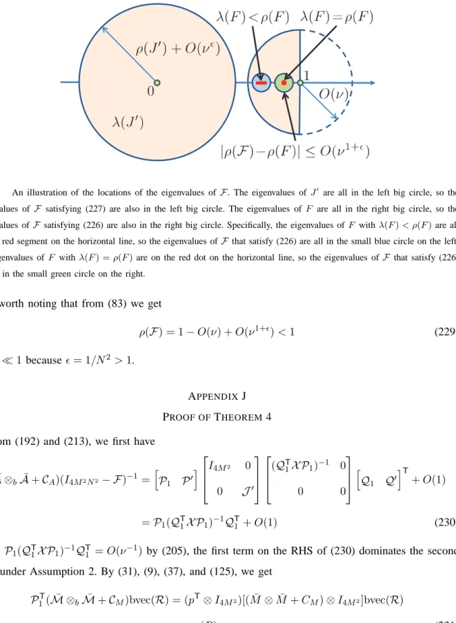
a more revealing MSD expression than (68) that is still accurate to the order of O(ν1+γo)_. A. Perron Eigenvectors

To proceed, we introduce the following condition on the matrix A¯_⊗A¯+CA.

Assumption 3 (Primitiveness of A¯_⊗A¯+CA): The matrixA¯⊗A¯+CAis assumed to be primitive [6,

p. 45], namely, that there exists a finite positive integer j such that all entries of ( ¯A_⊗A¯+CA)j are

positive.

Lemma 2 (Primitiveness of A¯): The matrix A¯ is primitive if A¯_⊗A¯+CA is primitive.

Proof: See Appendix F.

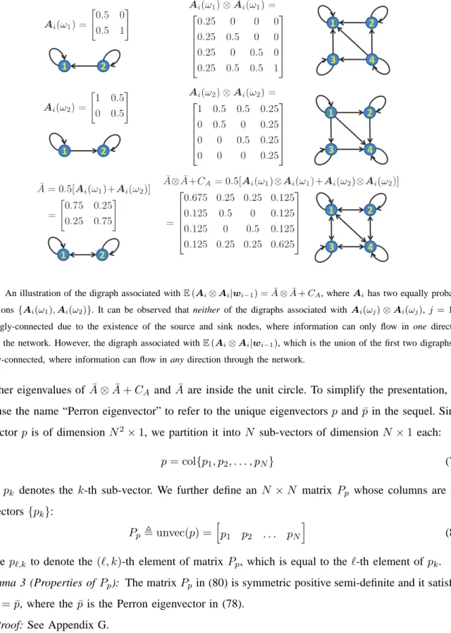
Assumption 3 is guaranteed if the directed graph (digraph) associated with the matrix A¯_⊗A¯+CA is

strongly-connected with as least one self-loop [6, pp. 30,34]. The digraph associated with A¯_⊗A¯+CA

is the union of all possible digraphs associated with the realizations ofAi⊗Ai [7, p. 29]. Each possible

digraph associated with Ai ⊗Ai is a Kronecker graph of order 2 generated by the initiator Ai [8].

Therefore, Assumption 3 amounts to an assumption that the union of all possible digraphs associated with the realizations of Ai ⊗Ai is strongly-connected with at least one self-loop. As illustrated in

Fig. 4, this condition still allows the digraphs associated withAi to be weakly-connected with or without

self-loops or even to be disconnected. Important cases such as random gossip [9]–[13] or probabilistic diffusion [14], [15] are therefore not ruled out by this condition. It can be verified that the converse of Lemma 2 is generally not true: when the digraph associated with A¯is primitive, the digraph associated with A¯_⊗A¯+CA does not even need to be connected.

By Lemma 3 from Part I [2] and the above Assumption 3, the matrixA¯_⊗A¯+CA is left-stochastic and

primitive. It follows from the Perron-Frobenius theorem [6] [16] that this matrix has a unique eigenvalue at one and a pair of eigenvectors_{1N2, p} with positive entries satisfying:

( ¯A_⊗A¯+CA)·p=p, pT·1N2 = 1 (77)

Likewise, the matrixA¯is also left-stochastic and primitive. It has a unique eigenvalue at one and a pair of eigenvectors_{1N,p¯} with positive entries satisfying:

¯

A_·p¯= ¯p, p¯T_·1

2 1 2 1 4 3 2 1 2 1 4 3 2 1 2 1 4 3

Fig. 4. An illustration of the digraph associated withE₍A_i⊗A_i|w_i−1) = ¯A⊗A¯+CA, whereAihas two equally probable realizations {Ai(ω1),Ai(ω2)}. It can be observed that neither of the digraphs associated withAi(ωj)⊗Ai(ωj), j = 1,2, is strongly-connected due to the existence of the source and sink nodes, where information can only flow in one direction through the network. However, the digraph associated withE(Ai⊗Ai|wi−1), which is the union of the first two digraphs, is

strongly-connected, where information can flow in any direction through the network.

All other eigenvalues ofA¯_⊗A¯+CA andA¯ are inside the unit circle. To simplify the presentation, we

shall use the name “Perron eigenvector” to refer to the unique eigenvectorsp andp¯in the sequel. Since the vectorp is of dimension N2_×1, we partition it into N sub-vectors of dimension N _×1 each:

p= col_{p1, p2, . . . , pN} (79)

where pk denotes the k-th sub-vector. We further define an N ×N matrix Pp whose columns are the

sub-vectors_{pk}: Pp ,unvec(p) = h p1 p2 . . . pN i (80) We use pℓ,k to denote the (ℓ, k)-th element of matrix Pp, which is equal to theℓ-th element ofpk.

Lemma 3 (Properties of Pp): The matrixPp in (80) is symmetric positive semi-definite and it satisfies

Pp1N = ¯p, where thep¯is the Perron eigenvector in (78).

From Lemma 3, we get the following useful relations: pℓ,k =pk,ℓ, N X k=1 pℓ,k = ¯pℓ, N X ℓ=1 pℓ,k = ¯pk (81) B. Low-Rank Approximation

We return to our earlier objective of seeking a low-rank factorization for the matrix(I4M2_N2− F∗)−1.

For this purpose, we first introduce the 4M2_×4M2 Hermitian matrix:

F , N X k=1 N X ℓ=1 pℓ,k[ ¯DTℓ ⊗D¯k+cµ,ℓ,k(HℓT⊗Hk)] (82) where D¯k is given by (32).

Lemma 4 (Spectral radius of F): The matrixFin (82) is stable if condition (23) is satisfied. Moreover,

ρ(F) = [1₋λmin(H)]2+O(ν2) = 1−O(ν) (83) where H, N X k=1 ¯ pkµ¯kHk (84)

It can be verified that _kH_k=O(ν) and the O(ν2_{) term in (83) is negligible by Assumption 2.} Proof: See Appendix H.

Lemma 5 (Low-rank approximation): Under Assumptions 2 and 3, it holds that

(I4N2_M2 − F)−1 = (p1T_N2)⊗(I4M2−F)−1+O(1) (85) (p1TN2)⊗(I4M2−F)−1=O(ν−1) (86)

Under Assumption 2 where ν _≪1, the term in (86) dominates theO(1) term in (85). Moreover,

ρ(_F) =ρ(F) +O(ν1+1/N2) (87) where the ρ(F) from (83) dominates the O(ν) term in (87).

Proof: See Appendix I.

In expression (82) we observe that the matrix F is dependent on the first and second-order moments of the random step-sizes, i.e., _{µ¯k} and {cµ,ℓ,k}, and is also dependent on the first and second order

moments of the random combination coefficient matrix, i.e., A¯ andCA, through the dependence on the

Perron eigenvectorp. Let us introduce two 4M2_×4M2 _matrices:

R,

N

X

k=1

Z ,unvec (I4M2−F)−1vec(R)

(89) where Rk is given by (10). Using (186)–(188) and (214) in Appendix I, we can verify that

kR_k=O(ν2), _kZ_k=O(ν) (90) Then, using Lemma 5, we can establish the following useful result about the structure of the steady-state network error covariance matrix.

Theorem 4 (Network error covariance matrix): In steady-state, the covariance matrix of the network

error

¯e

w_i′ from the long-term model (24) can be approximated by

lim i→∞ E ¯e w′_i ¯e w′∗_i = (1N1TN)⊗Z+O(ν1+γ ′ o) ₍₉₁₎ where Z is from (89), γ_o′ , 1 2min{2, γv} (92)

and the first term on the RHS is dominant.

Proof: See Appendix J.

According to Theorem 4, the (cross-) covariance matrices of_{

¯e

w_k,i′ _}, which are uniformly expressed by

E

¯e

w′_k,i

¯e

w′∗_ℓ,i= unvec(z_i(ℓ,k)) for all k andℓ according to (58), can be approximated byZ in steady-state. However, this result is useful only if Z is a valid complex-Hessian-type matrix.

Definition 1 (Complex-Hessian-type matrices): Let X be an M_×M positive semi-definite Hermitian matrix and let Y be an M _×M symmetric matrix. Then, a positive semi-definite block matrix of the form H,    X Y Y∗ XT   ≥0 (93)

will be referred to as a complex-Hessian-type matrix.

The following result explains the reason for introducing this definition.

Lemma 6 (Complex-Hessian-type covariance matrices): Let x denote an M _×1 zero-mean complex random vector and let Rx,Exx∗ andR′x,ExxT. Then, the covariance matrix of _¯x=T_¯(x) is given

by E ¯ x ¯ x∗=    E_xx∗ E_xxT E_(x∗₎T_x∗ _E(x∗₎T_xT   =    Rx Rx′ R_x′∗ RT x    (94)

and this matrix is a complex-Hessian-type matrix.

By Lemma 6, for any zero-mean complex random vector x, the covariance matrix of

¯

x=

¯

T_{(x) must}

be a complex-Hessian-type matrix. Therefore, in order to approximate _{unvec(z_i(ℓ,k))_} by Z according to (91), we establish the following useful result for the matrix Z.

Lemma 7 (Properties of Z): The matrix Z in (89) is a positive semi-definite complex-Hessian-type matrix.

Proof: See Appendix K.

Using (91) and Lemmas 6 and 7, we arrive at the following result for the covariance and cross-covariance matrices of the steady-state error vectors _{

¯e

w′_k,i} from the long-term model (24).

Corollary 1 (Covariance and cross-covariance matrices): The steady-state (cross-) covariance

matri-ces of individual errors_{

¯e

w_k,i′ _}from the long-term model (24) can be approximated by

lim i→∞ E ¯e w_k,i′ ¯e w′∗_ℓ,i=Z+O(ν1+γo′) ₍₉₅₎

for all k andℓ, where Z is given by (89) and is dominant due to (90), and γ_o′ is given by (92).

Proof: By Lemma 7, the Z is a complex-Hessian-type matrix. According to Lemma 6, it is a valid covariance matrix for complex random vectors obtained via the transform

¯

T_{(·). The approximation (95)}

then follows from Theorem 4.

C. Steady-State MSD

Using Corollary 1, we obtain two useful results about the steady-state MSD for asynchronous diffusion solutions.

Corollary 2 (Steady-state MSD): Based on the same assumptions as Theorem 4, the steady-state MSD

(either the network MSD in (66) or the individual MSD in (67)) can be approximated by MSDnet= 1 4Tr(H −1_{R) +O(ν}1+γo_{) (96)} MSDk= 1 4Tr(H −1_{R) +O(ν}1+γo_{) (97)}

where _{H, R_} are given by (84) and (88), respectively, γo is from (70), and Tr(H−1R) is of the order

ofν.

Proof: See Appendix L.

Corollary 3 (Clustered solutions): The steady-state relative MSD between any two agents k and ℓ, i.e.,E_{kwk,i−wℓ,ik}2_{, is negligible compared to their steady-state absolute MSD with respect tow}o_{, i.e.,}

lim i→∞

E_{kwk,i−wℓ,ik}2 _=O(ν1+γ′

o)≪max

where γ_o′ is given by (92).

Proof: First, from Corollary 1, we have lim i→∞ E_ke ¯ w′_{k,i− e} ¯ w′_ℓ,ik2 = lim i→∞ E_[ke ¯ w′_k,ik2+_ke ¯ w′_ℓ,ik2_{− e} ¯ w′∗_k,ie ¯ w′_ℓ,i−e ¯ w′∗_ℓ,ie ¯ w′_k,i] = Tr(Z) + Tr(Z)₋Tr(Z)₋Tr(Z) +O(ν1+γo′) =O(ν1+γo′) ₍₉₉₎

From Theorem 1 and using (99), we get

lim i→∞ E_ke ¯ w_{k,i− e} ¯ w_ℓ,ik2= lim i→∞ E_ke ¯ w_{k,i− e} ¯ w′_k,i+ _e ¯ w′_k,i−e ¯ w′_ℓ,i+ _e ¯ w′_{ℓ,i− e} ¯ w_ℓ,ik2 ≤ lim i→∞3 E _ke ¯ w_k,i− e ¯ w′_k,ik2+_ke ¯ w′_k,i−e ¯ w′_ℓ,ik2+_ke ¯ w′_ℓ,i− e ¯ w_ℓ,ik2 ≤O(ν2) +O(ν1+γ′o) +O(ν2) ≤O(ν1+γ′o) (100)

Using (6) from Part I [2], (100), and Corollary 2 completes the proof.

We illustrated Corollaries 2 and 3 earlier in Fig. 1. We note that if the cost functions, _{Jk(w)}, are

deterministic with known gradient vectors, then performance results in Corollaries 2 and 3 can still be deduced from our expressions by setting the gradient noise to zero.

V. CONCLUSION

We studied in some detail the MSE performance of asynchronous networks with random step-sizes, links, topologies, and combination coefficients. Assuming sufficiently small step-sizes, we showed that at steady-state, the error vector for every individual agent tends to cluster withinO(ν1+γo_{)from each other,}

which means that the MSD performance is essentially uniform across the entire network. The result in Corollary 2 shows explicitly how the MSD performance of the network is affected by the asynchronous behavior. Quantities that relate to the first and second-order moments of the distribution of the random step-sizes and combination coefficients appear in these expressions. These results can be used to guide strategies for adjusting the combination weights and the rate at which the agents update their solutions and to ensure that the performance (in terms of MSD and rate of convergence) does not degrade below desirable levels.

APPENDIXA PROOF OFLEMMA 1 Using Lemma 1 in Part I [2], we get from (14)–(15) that

kHk−Hk,i−1k= Z 1 0 [_∇2 ¯ w ¯ w∗Jk( ¯ wo)_{− ∇}2 ¯ w ¯ w∗Jk( ¯ wo₋t ¯e wk,i−1)]dt ≤ Z 1 0 k∇ 2 ¯ w ¯ w∗Jk( ¯ wo)_{− ∇}2 ¯ w ¯ w∗Jk( ¯ wo₋t ¯e wk,i−1)kdt ≤ Z 1 0 τ_k′ _·t_{· k} ¯e w_k,i−1kdt= τ_k′ 2 · kw¯ek,i−1k (101)

Using (101), we get from (18) that

kd_k,ik2 _≤[µ_k(i)]2_{· k}Hk−Hk,i−1k2· k ¯e w_k,i−1k2 ≤[µk(i)]2· τ_k′2 4 · kw¯ek,i−1k 4 ₍₁₀₂₎

Taking the expectation of both sides of (102) yields

E_kdk,ik2 _≤µ¯(2) k τ′2 k 4 ·Ekw¯ek,i−1k 4 ₍₁₀₃₎

From Theorem 2 of Part I [2], it holds for large enough ithat

E_kwek,ik4 _≤2b2

4·ν2 (104)

Using the fact from (198) of Part I [2] that µ¯(2)_{k ≤}ν2 _{for anyk, and letting}

τ′ ,max k τ

′

k (105)

we obtain from (103) and (104) that

E_kdk,ik2 _≤2τ′2_b2

4·ν4 =O(ν4) (106)

where a factor of 4 appeared due to the conversion

¯

T_{(·) from (4) of Part I [2]. Then,}

E_kAT idik2 = N X k=1 E X ℓ∈Nk,i aℓk(i)dℓ,i 2 (a) ≤ N X k=1 E   X ℓ∈N_k,i aℓk(i)kdℓ,ik2   = N X k=1 X ℓ∈Nk ¯ aℓkEkdℓ,ik2 ≤N _·max ℓ E_kdℓ,ik2

(b)

≤ 2N τ′2b2_4·ν4 (107)

where step (a) is by using Jensen’s inequality; and step (b) is by using (106).

APPENDIXB PROOF OFTHEOREM 1

We rewrite the original error recursion (16) and the long-term model (24) respectively as follows:

¯e

ψk,i= [I2M −µk(i)Hk] ¯e

wk,i−1+µk(i) ¯

vk,i(wk,i−1) +dk,i (108)

¯e w_k,i= X ℓ∈Nk,i a_ℓk(i) ¯e ψ_ℓ,i (109) and ¯e ψ_k,i′ = [I2M −µk(i)Hk] ¯e w′_k,i−1+µ_k(i) ¯ v_k,i(w_k,i−1) (110) ¯e w_k,i′ = X ℓ∈Nk,i aℓk(i) ¯ e ψ_ℓ,i′ (111)

with the prime notation for quantities associated with the long-term model (24). From (109) and (111), and using Jensen’s inequality, the squared 2-norm of the difference between the two models is given by

kw_¯ek,i− ¯e w_k,i′ _k2_≤ X ℓ∈Nk,i aℓk(i)k ¯e ψℓ,i− ¯e ψ′_ℓ,ik2 (112)

Taking the expectation of both sides yields

E_k ¯e wk,i− ¯e w_k,i′ _k2 _≤ X ℓ∈Nk ¯ aℓkEk ¯e ψℓ,i− ¯e ψ_ℓ,i′ _k2 ≤max ℓ E_k ¯ e ψℓ,i− ¯ e ψ′_ℓ,ik2 (113)

for all k. Then,

max k E_k ¯e wk,i− ¯e w_k,i′ _k2 _≤max k E_k ¯ e ψk,i− ¯ e ψ_k,i′ _k2 (114)

From (108) and (110), we have

¯e ψk,i− ¯e ψ_k,i′ = [I2M −µk(i)Hk]( ¯e wk,i−1− ¯e w′_k,i−1) +dk,i (115)

Taking the expected squared 2-norm of both sides, we have

E_k ¯e ψ_k,i− ¯e ψ_k,i′ _k2 _≤E_{k[I2M −µk(i)Hk](} ¯e w_k,i−1− ¯e w_k,i′ ₋₁) +d_k,ik2 =E (1−t) I2M −µk(i)Hk 1₋t (w¯ek,i−1−w¯e ′ k,i−1) +t d_k,i t 2

≤(1₋t)−1E_{kI2M −µk(i)Hkk}2_·E_k

¯e

w_k,i−1−

¯e

w′_k,i−1k2+t−1E_kdk,ik2 ₍₁₁₆₎

for any 0< t <1, where we used Jensen’s inequality in the second inequality. By condition (19), it can be verified that E_{kI2M −µk(i)Hkk}2 _≤1−2¯µ(1) k λk,min+ ¯µ (2) k λ2k,max (a) ≤ 1₋µ¯(1)_k λk,min ≤ 1₋1 2µ¯ (1) k λk,min 2 <1 (117)

where step (a) is from (192) of Part I [2]. Substituting t= 1₂µ¯(1)_k λk,min<1 and (117) into (116) yields E_k ¯e ψ_k,i− ¯e ψ_k,i′ _k2_≤ 1₋1 2µ¯ (1) k λk,min E_k ¯e w_k,i−1− ¯e w′_k,i−1k2+ 2 λk,minµ¯(1)_k E_kdk,ik2 ₍₁₁₈₎

Using (103), the second term on the RHS of (118) can be bounded for large enough iby

2 λk,minµ¯(1)_k ·E_kdk,ik2 _≤ 2 λk,minµ¯(1)_k ·µ¯(2)_k τ ′2 k 4 ·Ekw¯ek,i−1k 4 = τ ′2 k 2λk,min · ¯ µ(2)_k ¯ µ(1)_k · E_k ¯e wk,i−1k4 ≤ τ ′2 kν 2λk,min · E_k ¯e wk,i−1k4 (119)

where we used the fact from (200) of Part I [2] that ν_≥µ¯(2)_k /µ¯(1)_k . Substituting (119) into (118) yields

E_k ¯e ψ_k,i− ¯e ψ_k,i′ _k2 _≤ 1₋1 2µ¯ (1) k λk,min E_k ¯e w_k,i−1− ¯e w_k,i′ _−1k2+ τ ′2 kν 2λk,min E_k ¯e w_k,i−1k4 (120) Therefore, max k E_k ¯e ψk,i− ¯e ψ_k,i′ _k2 _≤max k 1₋1 2µ¯ (1) k λk,min max k E_k ¯e wk,i−1− ¯e w_k,i′ _−1k2 + max k τ_k′2ν 2λk,min · E_k ¯e wk,i−1k4 (121) Substituting (121) into (114) yields

max k E_k ¯e w_k,i− ¯e w_k,i′ _k2 _≤γ_·max k E_k ¯e w_k,i−1− ¯e w_k,i′ _−1k2+ τ ′2_ν 2 minkλk,min · max k E_k ¯e w_k,i−1k4 (122) where γ ,max k 1₋1 2µ¯ (1) k λk,min = 1₋1 2mink {µ¯ (1) k ·λk,min} (123)

When condition (19) holds, it can be verified by using (191) from Part I [2] that_|γ_|<1. Then, we get from (122) that lim sup i→∞ max k E_k ¯e w_k,i− ¯e w′_k,ik2 ≤ τ ′2_ν (1₋γ)_·2 minkλk,min · lim sup i→∞ max k E_k ¯e w_k,i−1k4

≤ 4τ ′2_b2

4ν3

minkµ¯(1)_k ·minkλ2_k,min

≤O(ν2) (124)

where we used Theorem 2 from Part I [2] and the fact from (198) of Part I [2] thatµ¯(1)_k =O(ν). APPENDIXC

BLOCKOPERATIONS

Consider a block matrix _X of sizeN M_×N M and partition it intoN_×N blocks whereXkℓ denotes

its (k, ℓ)-th sub-matrix of sizeM_×M. The block vectorization of_X with block size M_×M is defined as follows [17]:

bvec(_X)_,col_{vec(X11),vec(X21), . . . ,vec(XN1), . . . ,vec(X1N),vec(X2N), . . . ,vec(XN N)} (125)

Let_Y denote another block matrix of size N M_×N M and letYkℓ denote its(k, ℓ)-th sub-matrix of size

M_×M. Then, the block Kronecker product of _X and _Y with block sizeM _×M is defined by [17]:

X ⊗bY ,            Z11 Z12 . . . Z1N Z21 Z22 . . . Z2N .. . ... . .. ... ZN1 ZN2 . . . ZN N            (126) where Zkℓ ,            Xkℓ⊗Y11 Xkℓ⊗Y12 . . . Xkℓ⊗Y1N Xkℓ⊗Y21 Xkℓ⊗Y22 . . . Xkℓ⊗Y2N .. . ... . .. ... Xkℓ⊗YN1 Xkℓ⊗YN2 . . . Xkℓ⊗YN N            (127)

For any matrices _{X, Y, A, B_} of compatible dimensions and with blocks of size M_×M, it holds that

(X_⊗A)_⊗b(Y ⊗B) = (X⊗Y)⊗(A⊗B) (128)

where_⊗denotes the traditional Kronecker product operation. Other useful properties for the_⊗b operation

can be found in [17, pp. 176-179] and are listed here for ease of reference:

bvec(_ABC) = (_CT_⊗bA)·bvec(B) (129) bvec(xyT_{) =y⊗}

bx (130)

(_AC)_⊗b(BD) = (A ⊗bB)(C ⊗bD) (132)

(_A+_B)_⊗b(C+D) =A ⊗bC+B ⊗bC+A ⊗bD+B ⊗bD (133)

(_{A ⊗}bB)∗=A∗⊗bB∗ (134)

(_{A ⊗}bB)T=AT⊗bBT (135)

for any block matrices _{A,_B,_C,_D} and any block vectors _{x, y_} with appropriate sizes. APPENDIXD

PROOF OFTHEOREM 2 From the long-term model (41), we obtain that

E₍ ¯e w′_i ¯e w_i′∗_|F_{i−1) =}E₍B_i ¯e w_i′₋₁ ¯e w′∗_i−1B∗_i|F_{i−1) +}E₍ ¯si¯s ∗ i|Fi−1) (136)

where the cross terms that involve

¯ si disappear because E(Bi ¯e wi−1 ¯ s∗_i|F_{i−1) = 0 by (29) and (35).}

Performing the block vectorization of block size 2M for both sides of (136), and using (129) and (130) yield E_[( ¯e w_i′∗)T_⊗b ¯e w_i′_|F_{i−1] =}E_[(B∗_i)T_⊗bBi][( ¯e w_i′∗₋₁)T_⊗b ¯e w_i′₋₁] +E_[( ¯ s∗_i)T_⊗b ¯si|Fi−1] (137)

Using (29), (132), and (135), the second term on the RHS of (137) can be expressed as

E_[( ¯s ∗ i)T⊗b ¯si|Fi−1] = ( ¯A ⊗bA¯+CA) T_{( ¯M ⊗} bM¯ +CM)ri(wi−1) (138)

Substituting (51) and (138) into (137), taking the expectation with respect to F_{i−1, and then using (48),}

we arrive at the desired recursion (52), namely,

E_[( ¯e w′∗_i )T_⊗ b ¯e w′_i] =_F∗E_[( ¯e w′∗_i−1)T_⊗ b ¯e w′_i−1] +yi (139)

From (51), we know that _G in (50) is a factor of _F. Hence, we use the following result to examine the stability of _F.

Lemma 8 (Properties of G): The matrix G in (50) satisfies the following properties: 1) Block diagonal and Hermitian matrix: it holds that

G= diag_{G1, G2, . . . , GN} (140)

where Gℓ denotes the ℓ-th block on the diagonal of G with block size4M2N ×4M2N and Gℓ,k

denotes the k-th block on the diagonal of Gℓ with block size 4M2 ×4M2. The block Gℓ,k is

Hermitian and is given by

Gℓ,k ,D¯ℓT⊗D¯k+cµ,ℓ,k(HℓT⊗Hk) (142)

where D¯k is given by (32).

2) Norms and spectral radius: it can be verified that

ρ(_G) = max

k,m{(1−µ¯kλk,m)

2_+c

µ,k,kλ2k,m} (143)

where λk,m denotes them-th eigenvalue ofHk,m= 1,2, . . . ,2M.

3) Stability: if condition (23) holds, then

ρ(_G) <1 (144)

Proof: See Appendix E.

Using the fact that _G is block diagonal and Hermitian, and that A¯_⊗A¯+CA is block left-stochastic,

result (153) from [4, App. A] implies that

ρ(_F)_≤ρ(_G) (145)

By (144) and (145), we conclude that _F is stable if condition (23) holds.

APPENDIX E PROOF OFLEMMA 8

The first property relating to the block diagonal and Hermitian structure of (140)–(142) is established by using the definition of_⊗band (50). Because the matrixDiis block diagonal with block size2M×2M,

the block Kronecker product:

G_{i ,}DT_{i ⊗b}D_i (146)

is block diagonal with block size 4M2N _×4M2N and each block is itself block diagonal with block size4M2_×4M2. Let us denote the ℓ-th block on the diagonal ofG_i with block size 4M2N _×4M2N

by

Gℓ,i,DTℓ,i⊗Di (147)

and thek-th block on the diagonal ofGℓ,i with block size 4M2×4M2 by

where we used the fact that D_ℓ,i is Hermitian. Then, we have

G_i= diag_{G_1,i,G_2,i, . . . ,G_N,i} (149) Gℓ,i= diag{Gℓ,1,i,Gℓ,2,i, . . . ,Gℓ,N,i} (150)

Using (50) and taking the expectation of both sides of (149) and (150), we get (140) and (141) by identifying:

Gℓ =E[Gℓ,i], Gℓ,k =E[Gℓ,k,i] (151)

Equation (142) follows from (151), (148), (26), and (32). Since the matrices _{Gℓ,k} are all Hermitian,

by (140) and (141), the matrix _G is also Hermitian.

The second property in (143) is established by using the block diagonal and Hermitian properties of

G to readily conclude that ρ(_G) = maxℓ,kρ(Gℓ,k). Furthermore, by (142), the eigenvalues of Gℓ,k are

given by

λm,n(Gℓ,k) = (1−µ¯ℓλℓ,n)(1−µ¯kλk,m) +cµ,ℓ,kλℓ,nλk,m (152)

for any ℓ, k= 1,2, . . . , N, where λk,m denotes the m-th eigenvalue ofHk and m, n = 1,2, . . . ,2M. It

is straightforward to verify that

λm,n(Gℓ,k) =E[(1−µℓ(i)λℓ,n)(1−µk(i)λk,m)] (153)

Using Cauchy-Schwarz inequality, we get

|E_{[(1−µℓ(i)λℓ,n)(1−µk(i)λk,m)]| ≤}qE_{[(1−µℓ(i)λℓ,n)}2_]·E_{[(1−µk(i)λk,m)}2_] ≤max k,m{ E_{[(1−µk(i)λk,m)}2_]} = max k,m{(1−µ¯kλk,m) 2_+c µ,k,kλ2k,m} (154)

where the first inequality becomes equality when ℓ=kand n=m. From (152)–(154) we get

|λm,n(Gℓ,k)| ≤max

k,m{(1−µ¯kλk,m)

2_+c

µ,k,kλ2k,m} (155)

for any ℓ, k, m, and n. Since the above inequality applies to all eigenvalues of Gℓ,k, and since Gℓ,k is

Hermitian, we get

ρ(Gℓ,k)≤max

k,m{(1−µ¯kλk,m)

2_+c

µ,k,kλ2k,m} (156)

Furthermore, from (152) we know that

so that equality in (156) is achievable for some kand m.

For the third property in (144), we introduce the quadratic function

f(x),(1₋µ¯kx)2+cµ,k,kx2 (158)

with x_∈[λk,min, λk,max]. It is easy to verify that f(x) achieves its maximum value at either one of its

boundaries:

f(x)_≤max_{f(λk,min), f(λk,max)}

≤1₋2¯µkλk,min+ (¯µ2k+cµ,k,k)λ2k,max (159)

From Assumption 2 in Part I [2] we have λk,min ≤λk,m ≤λk,max for any k and m. We then deduce

from (159) that

f(λk,m)≤1−2¯µkλk,min+ (¯µ2k+cµ,k,k)λ2k,max (160)

for anyk andm. Using (143), (158), and (160), we get

ρ(_G) = max k,m{f(λk,m)} ≤max k {f(λk,min), f(λk,max)} <max k {f(λk,min), f(λk,max)}+α(¯µ 2 k+cµ,k,k) (161)

where α >0 by Assumption 1. When condition (23) holds, using (144) from Part I [2], we have

max

k {1−2¯µkλk,min+ (¯µ

2

k+cµ,k,k)(λ2k,max+α)}<1 (162)

Therefore, by (161) and (162), if condition (23) holds, then ρ(_G)<1, which completes the proof. APPENDIXF

PROOF OFLEMMA 2

From Lemma 3 in Part I [2] we know that the matrices A¯_⊗A¯+CA and A¯ are both left-stochastic.

To establish the desired result, we only need to show that the matrix A¯_⊗A¯is primitive if A¯_⊗A¯+CA

is primitive. This is because if A¯_⊗A¯is primitive, then for some finite positive integerj >0, the matrix

( ¯A_⊗A¯)j _{has strictly positive entries. Since ( ¯A⊗A}¯₎j _{= ¯A}j _⊗A¯j _{and A}¯ _{has nonnegative entries, A}¯j

must have strictly positive entries. Therefore, A¯ is primitive.

In order to prove that the matrix A¯_⊗A¯is primitive if A¯_⊗A¯+CA is primitive, we first introduce the

Definition 2 (Comparing sparsity): For any two matrices _{A, B_} with nonnegative entries and of the same size, the matrix A is called sparser than B, or, equivalently, B is called denser than A, if, and only if, [B]ℓk >0 whenever[A]ℓk >0 for anyk andℓ.

It is straightforward to verify the following three useful properties related to Definition 2.

Lemma 9 (Denser product): For any M _×N matrices _{A, B_} and any N _×P matrices _{C, D_} all with nonnegative entries, ifB is denser thanA andD is denser thanC, thenBD is denser than AC.

Lemma 10 (Denser Kronecker product): For any M _×N matrices _{A, B_} and any P _×Q matrices

{C, D_} all with nonnegative entries, ifB is denser thanAandDis denser thanC, thenB_⊗Dis denser than A_⊗C.

Lemma 11 (Sum is not denser): For any set of M_×N matrices_{Ai}with nonnegative entries, where

i _{∈ I} and _I is an index set (which can be uncountable), if there exists an M _×N matrix B with nonnegative entries such thatB is denser than everyAi,i∈ I, and assuming that the sumS ,Pi∈IAi

exists, then B is also denser than S.

Now, from Lemma 2 in Part I [2], we know that A¯ is denser than any realization of A_i, say, A_i(ω)

where ω _∈ Ω and Ω is the sample space of A_i. Using Lemma 10, we get that A¯_⊗A¯ is denser than anyA_i(ω)_⊗A_i(ω). Using Lemma 11 and the fact that the probability measures only take nonnegative values, we get thatA¯_⊗A¯ is denser thanA¯_⊗A¯+CA=E[Ai⊗Ai]. IfA¯⊗A¯+CA is primitive, then

there exists a finite positive integer j >0 such that ( ¯A_⊗A¯+CA)j has strictly positive entries. Using

Lemma 9, we know that( ¯A_⊗A¯)j must be denser than( ¯A_⊗A¯+CA)j. Therefore,( ¯A⊗A¯)j must also

have strictly positive entries, which means that A¯_⊗A¯ must be primitive. APPENDIXG

PROOF OFLEMMA 3 We first show that Pp =PpT, or equivalently,

p= vec(PT

p) (163)

Lemma 12 (Vec-permutation matrix): The N2 _{× N}2 _{vec-permutation matrix Π is a matrix whose}

columns are formed from the basis vectors in RN2

and it satisfies:

vec(A) = Π_·vec(AT_{) (164)}

for anyN _×N matrixA. Then, for anyN _×N matrices_{A, B_},

In addition,Π = ΠT_{= Π}∗ _{= Π}−1_.

Proof: See [18, Tabs. I and II] [19, Eqs. (5) and (6)].

Let Π be the permutation matrix that satisfies

vec(P_pT) = Π_·vec(Pp) (166)

From (80) and (166), proving (163) is equivalent to proving

p= Π_·p (167)

To establish (167), we only need to show that Π_·p is the Perron eigenvector of A¯_⊗A¯+CA. In that

case, we can obtain (167) directly from the uniqueness of the Perron eigenvector, which is p. Thus, note that

Π( ¯A_⊗A¯+CA)Π = Π[E(Ai⊗Ai]Π

(a)

= E_(Ai⊗Ai)

= ¯A_⊗A¯+CA (168)

where step (a) is by (165). Then, we deduce from (77) that

Π_·p= Π( ¯A_⊗A¯+CA)p= ( ¯A⊗A¯+CA)(Π·p) (169)

1TN2·Π·p=1T_N2 ·p= 1 (170)

where we used the fact that Π2 _{= I}

N2 by Lemma 12 and Π·1_N2 = 1_N2. Results (169) and (170)

establish that Π_·p is the Perron eigenvector of A¯_⊗A¯+CA and proves (167).

We next establish that Pp is positive semi-definite. Note that for any vectorx∈RN:

xTPpx= vec(xTPpx) = 1

N2(xT⊗xT)p·1TN21N2 (171)

by using (80) and the fact that 1TN21N2 = N2. Since A¯⊗A¯+C_A = E(A_j ⊗A_j), we can introduce

a series of fictitious random combination matrices _{A′_j;j _≥1_} such that they are mutually-independent and satisfy E_(A′

j⊗A′j) = ¯A⊗A¯+CA for anyj≥1. Let Φi,

Qi

j=1A′j for anyi≥1. Then, lim

i→∞

E_(Φi⊗Φi)(_{= lim}a)

i→∞ i Y j=1 E_(A′ j⊗A′j) = lim i→∞( ¯A⊗ ¯ A+CA)i (b) = p_·1T N2 (172)

where step (a) is by using the fact that the_{A′_j} are mutually-independent, and step (b) is by using the Perron-Frobenius Theorem [6]. Substituting (172) into (171) and using the fact that 1N2 = 1_N ⊗1_N,

we get xTPpx= 1 N2 _ilim_→∞E[(xTΦi1N) 2_] ≥0 (173)

which shows that Pp is positive semi-definite.

Now we show that Pp1N = ¯p. Note from (80) and (77) that

Pp =E[Ai·Pp·ATi ] (174)

by switching the order of unvec(_·) and E_{(·) and applyingunvec(·) to the identity vec(ABC) = (C}T_⊗

A)_·vec(B). Furthermore, we get from (174) that

Pp·1N =E(AiPpAiT)·1N = ¯A(Pp·1N) (175)

which implies that the vector Pp·1N is the Perron eigenvector of A¯, which is p¯. Because the Perron

eigenvector is unique, by (78), equation Pp·1N = ¯p must hold.

APPENDIXH PROOF OFLEMMA 4

We first establish that F is stable if condition (23) is satisfied. From (142) and (82), we get

F = N X ℓ=1 N X k=1 pℓ,kGℓ,k (176)

By (77) and (80), the elements _{pℓ,k} ofPp satisfy: N X ℓ=1 N X k=1 pℓ,k = 1, and pℓ,k >0 (177)

Then, in terms of the 2-induced norm, we have

kF_k(_≤a) N X k=1 N X ℓ=1 pℓ,kkGℓ,kk (b) ≤ max k,ℓ kGℓ,kk (c) = ρ(_G) (178)

where step (a) is from the triangle inequality of norms; step (b) is by using (177); and step (c) is by (143). Using (144), (178), and the fact that ρ(F) =_kF_k for the Hermitian matrix F, we conclude that matrix F is stable if condition (23) holds.

We now establish expression (83). Introduce the Hermitian matrix

F′ , N X k=1 N X ℓ=1 ¯ pℓp¯k( ¯DℓT⊗D¯k) (179)

From (32), we can rewriteF′ asF′ = (I2M−H)T⊗(I2M−H), where we used (78) and (84). Therefore,

the eigenvalues of F′ are equal to the products of any two of the eigenvalues of I2M −H, which are

given by1₋λ(H). Since _{p¯k}and{µ¯k} are all positive and{Hk} are all positive definite, it is easy to

verify that H in (84) is also positive definite. Then, from (84), (78), and (15), and using (8) from Part I [2] as well as Jensen’s inequality [20], we get

0< λ(H)_{≤ k}H_{k ≤}max

k {µ¯kλk,max} (180)

for all eigenvalues of H. When condition (23) holds, we get from (195) of Part I [2] that

¯ µk≤ ¯ µ(2)_k ¯ µk < λk,min λ2 k,max+α < 1 λk,max (181) for any k. This implies that maxk{µ¯kλk,max} <1 and therefore, 0 < λ(H) <1 for all eigenvalues of

H. From (84) and (186), we obtain

0< λ(H) =O(ν)<1 (182) for any eigenvalue of H. Therefore, we get

λ(I2M −H) = 1−O(ν), ρ(I2M −H) = 1−λmin(H) (183)

where λmin(·) denotes the smallest eigenvalue of its Hermitian matrix argument. We further get from

(183) that

λ(F′) = 1₋O(ν), ρ(F′) = [1₋λmin(H)]2 (184)

Using Lemma 3, (77), (78), and (32), the difference between F in (82) andF′ in (179) is given by

F ₋F′= N X k=1 N X ℓ=1 {[(pℓ,k−p¯ℓp¯k)¯µℓµ¯k+pℓ,kcµ,ℓ,k](HℓT⊗Hk)} (185)

which is also Hermitian. From (198) in Part I [2], we get

¯

µk≡µ¯(1)k ≤ν (186)

cµ,k,k ≤µ¯(2)_k ≤ν2 (187)

|cµ,ℓ,k| ≤√cµ,ℓ,ℓ·cµ,k,k ≤ν2 (188)

where (188) is by using the Cauchy-Schwartz inequality. By (186)–(188), we get _kF ₋F′_k = O(ν2). Using a corollary of the Wielandt-Hoffman theorem [21, Corollary 8.1.6, p. 396], we then conclude that

whereλm(·)denotes them-th eigenvalue of its Hermitian matrix argument; the eigenvalues are assumed

to be ordered from largest to smallest in each case. Result (189) implies that for every eigenvalue ofF′

there is an eigenvalue of F that is O(ν2) close to it. From (189) and (184) we immediately deduce that

λm(F) = 1−O(ν), ρ(F) =ρ(F′) +O(ν2) (190)

where ρ(F′) from (184) dominates theO(ν2) term. APPENDIXI PROOF OFLEMMA 5 We first establish (85). Introduce the Jordan decomposition:

¯ A_⊗A¯+CA,P JQT= h p P′ i    1 0 0 J′    h 1N2 Q′ iT (191)

where J is the Jordan canonical form of A¯_⊗A¯+CA andJ′ is a sub-matrix of J containing its stable

eigenvalues, P′ and Q′ are sub-matrices of P and Q, and P−1 _=QT_{. Then, the Jordan decomposition}

of_{A ⊗}¯ bA¯+CA is given by ¯ A ⊗bA¯+CA=PJ QT= h P1 P′ i    I4M2 0 0 _J′    h Q1 Q′ iT (192) where P ,P _⊗I4M2, P′ ,P′⊗I_4M2 (193) J ,J_⊗I4M2, J′ ,J′⊗I_4M2 (194) Q,Q_⊗I4M2, Q′ ,Q′⊗I_4M2 (195) P1 ,p⊗I4M2, Q₁,1_N2⊗I_4M2 (196) Let X ,I4M2_N2 − G (197)

where _G is given by (50). Then, by (51),

QTFP=_QT[_{G ·}( ¯_{A ⊗}bA¯+CA)]P =_QT_(I

4M2_N2− X)(PJ QT)P =_{J − Q}T_{X PJ}

=    I4M2 − QT₁X P₁ −QT₁X P′J′ −Q′T_{X P} 1 J′− Q′TX P′J′    (198)

From (198), we further get

(I4M2_N2 − QTFP)−1 =    QT 1X P1 QT1X P′J′ Q′T_{X P} 1 I− J′+Q′TX P′J′    −1 (199)

where the I denotes the 4M2(N2₋1)_×4M2(N2₋1) identity matrix. The quantity _QT_{1X P}1 in (198)

can be expressed as QT1X P1 (a) = _QT_{1 · P}1− QT1GP1 (b) = (1TN2p)⊗I4M2−(1T_N2⊗I4M2)(diag{G_ℓ,k})(p⊗I_4M2) (c) = I4M2−F (200)

where step (a) is by (197); step (b) is by (140)–(141); and step (c) is by (176). We already know that the matricesF and_F are stable for sufficiently small step-sizes. Thus, the matricesI4M2_N2−F andI_4M2−F

are invertible. It follows that the quantity _QT_{1X P}1 is invertible. Moreover, the Schur complement with

respect to _QT_{1X P}1 in (199) is also invertible. Let us denote the inverse of this Schur complement by

∆,[I_{− J}′+_Q′T_{X P}′

J′− Q′T_{X P}

1(QT1X P1)−1QT1X P′J′]−1 (201)

Then, by using a formula for the inversion of block matrices [22, Eq. (7), p. 48], equality (199) can be expressed as (I4M2_N2− QTFP)−1 =    (_QT 1X P1)−1+ ∆′ −(QT1X P1)−1QT1X P′J′∆ −∆_Q′T_{X P} 1(QT1X P1)−1 ∆    (202) where ∆′,(_QT_{1X P}1)−1QT1X P′J′∆Q′TX P1(QT1X P1)−1 (203)

Now, from (200), (82), (32), (81), and (84), we can also write

QT1X P1=H⊗I2M +I2M ⊗H− N

X

ℓ,k=1

pℓ,k(¯µℓµ¯k+cµ,ℓ,k)(HℓT⊗Hk) (204)

It follows from (204) and (186)–(188) that _QT_{1X P}1 is Hermitian and

kQT