Mining and Managing Large-Scale Temporal Graphs

UC Santa Barbara Electronic Theses and Dissertations

Mining and Managing Large-Scale Temporal Graphs Permalink https://escholarship.org/uc/item/3r65p6nh Author Zong, Bo Publication Date 2015 Peer reviewed|Thesis/dissertation

Santa Barbara

Mining and Managing Large-Scale Temporal Graphs

A Dissertation submitted in partial satisfaction of the requirements for the degree of

Doctor of Philosophy in Computer Science by Bo Zong Committee in Charge:

Professor Ambuj K. Singh, Co-Chair Professor Xifeng Yan, Co-Chair Professor Subhash Suri

Professor Xifeng Yan, Co-Chair

Professor Subhash Suri

Professor Ambuj K. Singh, Committee Chair

Copyright © 2015 by

that make me happy everyday, lend me courage to explore unknown world, and lead me to where I am.

First of all, I would like to express my sincere gratitude to my advisors, Prof. Ambuj K. Singh and Prof. Xifeng Yan. I am fortunate to work with two great advisors who give me invaluable guidance on my research path and also grant me freedom to explore independent work. In my five years’ PhD study, I have learned how to perform good research from my advisors’ enthusiasm, immense knowledge, and patience. Outside of academia, Ambuj and Xifeng are also the advisors in my life. They share with me the wisdom of how to live a happy, healthy, and meaningful life, and give me great support and encouragement.

Second, I sincerely thank my committee member Prof. Subhash Suri. I am deeply grateful for his valuable feedback and insightful suggestions on my work.

My sincere thanks also go to Prof. Yinghui Wu and Dr. Misael Mongiov`ı. It is my great pleasure to work with them on multiple interesting projects. I am also grateful to Dr. Nan Li, Dr. Kyle Chipman, Dr. Arijit Khan, Prof. Petko Bogdanov, Dr. Nicholas D. Larusso, and Prof. Sayan Ranu for their various forms of help during my PhD study.

I am indebted to all my labmates: Dr. Shengqi Yang, Dr. Xuan-Hong Dang, Dr. Yang Li, Minh X. Hoang, Huan Sun, Arlei Lopes da Silva, Victor Amelkin, Fangqiu Han, Sourav Medya, Honglei Liu, Anh Nguyen, Yu Su, Haraldur Hall-grimsson, Izzeddin G¨ur, Theodore Georgiou, Semih Yavuz, and Hongyuan You.

I would like to acknowledge my collaborators and mentors for their valuable advice and numerous discussions: Dr. Ramya Raghavendra, Dr. Mudhakar Sri-vatsa, Dr. Christos Gkantsidis, Dr. Milan Vojnovic, Dr. Zhichun Li, Dr. Xusheng Xiao, Dr. Zhenyu Wu, and Prof. Zhiyun Qian.

Zong and my mother Qiandi Shao for their endless love, and for always being there for me. Thanks to my wife Dr. Xiaohan Zhao for her unconditional love, support, and encouragement.

Bo Zong

Education

2015 Ph.D in Computer Science, University of California, Santa Barbara. 2010 Master of Science in Computer Science, Nanjing University, China. 2007 Bachelor of Science in Computer Science, Nanjing University, China.

Experience

08/2010 – 09/2015 Research Assistant, University of California, Santa Barbara. 03/2015 – 06/2015 Teaching Assistant, University of California, Santa Barbara. 06/2015 – 07/2015 Research Mentor, University of California, Santa Barbara. 06/2014 – 09/2014 Research Intern, NEC Labs America, Princeton, NJ, USA. 05/2013 – 08/2013 Research Intern, Microsoft Research, Cambridge, UK.

06/2012 – 09/2012 Research Intern, IBM Research T. J. Watson, Yorktown Heights, NY, USA.

Publication

(Publications marked with ’*’ order authors alphabetically.)

Bo Zong, Christos Gkantsidis, and Milan Vojnovic. “Herding ‘Small’ Streaming

Queries”. International Conference on Distributed Event-Based Systems (DEBS), July 2015.

Xifeng Yan. “Towards Scalable Critical Alert Mining”. ACM SIGKDD Conference on Knowledge Discovery and Data Mining (KDD), Aug. 2014.

Bo Zong, Ramya Raghavendra, Mudhakar Srivatsa, Xifeng Yan, Ambuj K. Singh,

and Kang-Won Lee. “Cloud Service Placement via Subgraph Matching”. International Conference on Data Engineering (ICDE), Apr. 2014.

Bo Zong, Yinghui Wu, Ambuj K. Singh, and Xifeng Yan. “Inferring the Underlying

Structure of Information Cascades”. International Conference on Data Mining (ICDM), Dec. 2012.

Shengqi Yang, Xifeng Yan, Bo Zong, and Arijit Khan. “Towards Effective Partition Management for Large Graphs”. ACM SIGMOD International Conference on Manage-ment of Data (SIGMOD), May. 2012.

Misael Mongiovi, Konstantinos Psounis, Ambuj K. Singh, Xifeng Yan, and Bo Zong. *“Efficient Multicasting for Delay Tolerant Networks using Graph Indexing”. Annual International Conference on Computer Communications (INFOCOM), Mar. 2012.

Bo Zong, Feng Xu, Jun Jiao, and Jian Lu. “A Broker-assisting Trust and Reputation

System Based on Artificial Neural Network”. International Conference on Systems, Man and Cybernetics (SMC), Oct. 2009.

Mining and Managing Large-Scale Temporal Graphs

by

Bo Zong

Large-scale temporal graphs are everywhere in our daily life. From online social networks, mobile networks, brain networks to computer systems, entities in these large complex systems communicate with each other, and their interac-tions evolve over time. Unlike traditional graphs, temporal graphs are dynamic: both topologies and attributes on nodes/edges may change over time. On the one hand, the dynamics have inspired new applications that rely on mining and man-aging temporal graphs. On the other hand, the dynamics also raise new technical challenges. First, it is difficult to discover or retrieve knowledge from complex temporal graph data. Second, because of the extra time dimension, we also face new scalability problems. To address these new challenges, we need to develop new methods that model temporal information in graphs so that we can deliver useful knowledge, new queries with temporal and structural constraints where users can obtain the desired knowledge, and new algorithms that are cost-effective for both mining and management tasks.

In this dissertation, we discuss our recent works on mining and managing large-scale temporal graphs.

First, we investigate two mining problems, including node ranking and link prediction problems. In these works, temporal graphs are applied to model the

data mining tasks that extract knowledge from temporal graphs. The discovered knowledge can help domain experts identify critical alerts in system monitoring applications and recover the complete traces for information propagation in online social networks. To address computation efficiency problems, we leverage the unique properties in temporal graphs to simplify mining processes. The resulting mining algorithms scale well with large-scale temporal graphs with millions of nodes and billions of edges. By experimental studies over real-life and synthetic data, we confirm the effectiveness and efficiency of our algorithms.

Second, we focus on temporal graph management problems. In these study, temporal graphs are used to model datacenter networks, mobile networks, and subscription relationships between stream queries and data sources. We formu-late graph queries to retrieve knowledge that supports applications in cloud ser-vice placement, information routing in mobile networks, and query assignment in stream processing system. We investigate three types of queries, including subgraph matching, temporal reachability, and graph partitioning. By utilizing the relatively stable components in these temporal graphs, we develop flexible data management techniques to enable fast query processing and handle graph dynamics. We evaluate the soundness of the proposed techniques by both real and synthetic data.

Through these study, we have learned valuable lessons. For temporal graph mining, temporal dimension may not necessarily increase computation complex-ity; instead, it may reduce computation complexity if temporal information can be wisely utilized. For temporal graph management, temporal graphs may include relatively stable components in real applications, which can help us develop

Curriculum Vitæ vii

List of Figures xvii

List of Tables xxi

1 Introduction 1

1.1 Mining Temporal Graphs. . . 5

1.2 Managing Temporal Graphs . . . 7

1.3 Contributions . . . 10

1.4 Thesis Organization. . . 12

2 Node Ranking in Temporal Graphs 13 2.1 Introduction . . . 13

2.2 Problem definition . . . 16

2.3 Mining framework. . . 21

2.4 Bound and pruning algorithm . . . 23

2.4.1 Pruning and verification . . . 26

2.4.2 Upper bound . . . 26 2.4.3 Lower bound . . . 29 2.4.4 Algorithm BnP . . . 30 2.5 Tree approximation . . . 32 2.5.1 Single-tree approximation . . . 32 2.5.2 Multi-tree sampling . . . 33

2.6.2 Case study. . . 38

2.6.3 Overall performance evaluation . . . 39

2.6.4 Performance evaluation of BnP . . . 41 2.6.5 Performance evaluation of MTS . . . 42 2.6.6 Scalability . . . 44 2.6.7 Summary . . . 45 2.7 Related work . . . 45 2.8 Summary . . . 47

3 Link Prediction in Temporal Graphs 48 3.1 Introduction . . . 48

3.2 Consistent Trees . . . 52

3.2.1 Consistent trees . . . 54

3.2.2 Cascade inference problem . . . 55

3.3 Cascades as perfect trees . . . 57

3.3.1 Bottom-up searching algorithm . . . 58

3.4 Cascades as bounded trees . . . 64

3.5 Experiment . . . 68

3.6 Related work . . . 75

3.7 Summary . . . 77

4 Subgraph Matching in Temporal Graphs 80 4.1 Introduction . . . 80 4.2 Problem definition . . . 83 4.3 An overview of Gradin . . . 85 4.4 Fragment index . . . 88 4.4.1 Naive solutions . . . 88 4.4.2 FracFilter construction . . . 91 4.4.3 Searching in FracFilter . . . 93

4.5.1 Minimum fragment cover . . . 99

4.5.2 Fingerprint based pruning . . . 101

4.6 Experiments . . . 103 4.6.1 Experiment setup . . . 104 4.6.2 Query processing . . . 107 4.6.3 Indexing performance. . . 111 4.6.4 Scalability . . . 114 4.6.5 Summary . . . 116 4.7 Related Work . . . 117 4.8 Summary . . . 120 5 Temporal Reachability 121 5.1 Introduction . . . 121 5.2 Preliminaries . . . 125 5.3 Problem Statement . . . 127 5.3.1 ILP formulation . . . 130

5.3.2 A naive approach for the demand cover problem . . . 132

5.3.3 A compact graph representation . . . 133

5.4 An indexing system for the demand cover problem. . . 135

5.4.1 Index structure . . . 136 5.4.2 Preprocessing . . . 137 5.4.3 Filtering . . . 139 5.4.4 Optimization . . . 144 5.4.5 Adaptive extension . . . 144 5.5 Experiment . . . 145 5.5.1 Dataset . . . 145 5.5.2 Implementation . . . 146 5.5.3 Response time . . . 147

5.5.7 Communication cost . . . 153

5.6 Related Work . . . 154

5.7 Summary . . . 155

6 Partitioning in Temporal Graphs 157 6.1 Introduction . . . 157

6.2 System Model and Assumptions . . . 162

6.2.1 Query Assignment Problem . . . 163

6.3 Hardness and Benchmark . . . 165

6.3.1 NP Hardness . . . 165

6.3.2 Random Query Assignment . . . 167

6.4 Offline Query Assignment . . . 169

6.4.1 Multi-Source Query Assignment . . . 169

6.4.2 Single-Source Query Assignment. . . 176

6.5 Online Query Assignment . . . 180

6.5.1 Greedy Online Algorithms . . . 180

6.5.2 Discussion . . . 183 6.6 Experiment . . . 187 6.6.1 Synthetic Workloads . . . 187 6.6.2 Real-World Workloads . . . 197 6.7 Related Work . . . 198 6.8 Summary . . . 200 7 Conclusion 201 7.1 Summary . . . 201 7.2 Lessons . . . 204 7.3 Future Work . . . 205

7.3.1 Data Analytics for Enterprise System Security . . . 205

2.1 Critical alert mining: pipeline . . . 17

2.2 AlgorithmBnP: Upper and lower bound . . . 29

2.3 The pruning procedure Prune . . . 31

2.4 AlgorithmMTS . . . 35

2.5 Critical alerts over LM . . . 39

2.6 Mining performance on LMalert graphs . . . 40

2.7 BnPperformance on LM alert graphs . . . 41

2.8 MTS performance onLM alert graphs . . . 43

2.9 Scalability results on SYNgraphs . . . 44

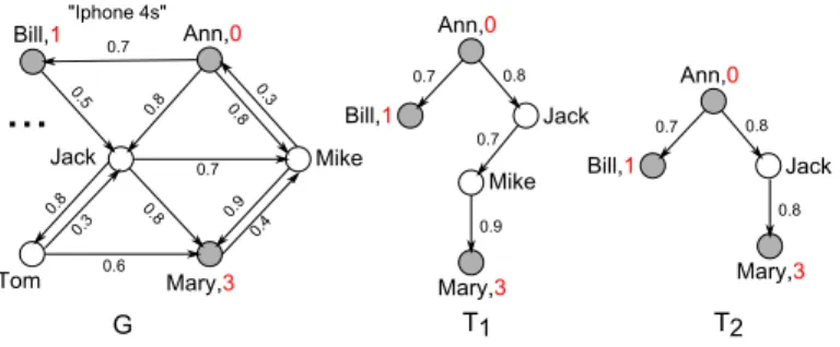
3.1 A cascade of an Ad (partially observed) in a social networkGfrom user Ann, and its two possible tree representations T1 and T2. . . 49

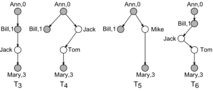
3.2 Tree representations of a partial observation X = {(Ann,0), (Bill,1), (Mary,3)_}: T3, T4 and T5 are consistent Trees, while T6 is not. . . 52

3.3 AlgorithmWPCT: initialization, pruning and local searching . . . 60

3.4 The bottom-up searching in the backbone network. . . 62

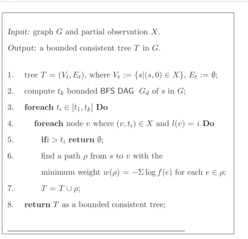
3.5 Algorithm WBCT: searching bounded consistent trees via top-down strategy . . . 66

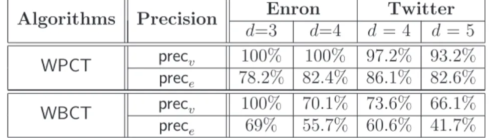
3.6 Theprec and rec of the inference algorithms over Enron email cas-cades and Retweet cascas-cades . . . 78

4.2 A fragment with its canonical labeling (top right) and fragment

coordinates (bottom right) . . . 85

4.3 Gradin consists of two parts: (1) offline index building and (2) online query processing . . . 86

4.4 FracFiltersof density 2 (left) and 4 (right): sin the top right corner is the structure of _Ds, points are label coordinates, and the integer in each grid is the grid id. . . 91

4.5 The Algorithm sketch for constructing a FracFilter . . . 93

4.6 The same query fragment (the red dot) requests fragment searching on two FracFilters of density 2 (left) and 4 (right). . . 94

4.7 An update on FracFilter of density 2 (left) and 4 (right), respec-tively. When a fragment in bottom left corner is updated, it triggers a bounded event on the left, but a migration event on the right. . . 98

4.8 An example of fingerprint based pruning . . . 102

4.9 Query processing performance on B3000 and CAIDA with 100 com-patible subgraphs returned. . . 105

4.10 Query processing on B3000 returning 5 or 10 matches . . . 109

4.11 Update processing time on B3000 and CAIDA . . . 113

4.12 Scalability on BCUBE graphs of 5K - 15K nodes. . . 115

5.1 An example of a DTN among moving nodes. (a) The four solid lines represent four trajectories. To simplicity we use the x-axis indicating the time. The big dashed circles represent the radio range of nodes. Nodes that are involved in a transition (contact beginning or contact end) are filled. Three data needs (r1, r2 and r3) are represented with filled triangles. Their deadlines are ta, t2 and t3, respectively while their latencies areδa,δ2 and δ3, respectively. (b) The corresponding temporal graph. Snapshots of the connectivity graph at three different times are depicted within big ovals. Temporal links joining contiguous snapshots are represented with dotted lines. . . 125

nodes j1, j2, . . . , j5 in the right-hand side are associated to elements.

The dashed circle delimits the radio range, of length d. Moving nodes follow the trajectories depicted by solid lines. The minimal sub-family that covers all destinations is {S2, S4}, corresponding to points p2,p4. . 130

5.3 The compressed graph representation of the example in Figure 5.1. A compressed graph is depicted over the space-time graph. Boxes and solid lines represent vertices and edges of the compressed graph, respec-tively. The extent of a box in time represents the component lifetime. Three data needs are represented (by filled triangles) with their extent in time. From left to right: ra = (2, ta, δa),rb = (3, tb, δb),rc = (4, tc, δc). 134

5.4 (a) An example of PIE graph. The small circles and thin arrows form the compressed graph. Each path is circumscribed by an oval and its lifetime is reported. Links between paths are represented by thick arrows. They are labeled by the ends of the lifetimes of their source vertices. Solid triangles within circles represent data needs. (b) Validity intervals of a set of data needs in a path p3. Bars represent the extent

of validity intervals of data needs. The minimal family of sets for this path is _{C(p3, ta), C(p3, tb)}. . . 138

5.5 An example of maximal coverage sets in a path. Bars represent the extent of validity intervals of data needs. The coverage of the time instants t1, t2 and t3 are maximal sets among all the coverage sets in

the path. The family of maximal sets can be found by sliding a vertical line in reverse time order and taking each time instant that corresponds to the beginning of a validity interval (indicated by the symbol “-” at the top) that occurs right after the end of the same or another validity interval (indicated by the symbol “+”). This family has minimum size. 143 5.6 Performances as functions of the size of the dataset (number of days) and the number of data needs. . . 148 5.7 Scalability over query size . . . 149 5.8 Preprocessing time and index size produced by CIDP on different datasets. The first row refers to CAB, the second row refers to GeoLife and the last row refers to SYN. . . 150 5.9 Evaluation of filtering capability. The first row refers to CAB, the second row refers to GeoLife and the last row refers to SYN. . . 152

6.1 Example of events flowing from the event sources to the query evaluators, and finally to users. In addition to global events, there are also personalized event sources; in this example, a query combines traffic updates with calendar events to generate notifications for the user (e.g., time to leave to be on time for next appointment given current traffic). Note that as user queries can dynamically come and go, the data flow

graph is temporal. . . 159

6.2 2-approximation for single-source QA. . . 177

6.3 Greedy algorithms for onlineQA. . . 181

6.4 Performance of offline query assignment. . . 190

6.5 Performance of online query assignment without query departures. 190 6.6 Performance of online algorithms with dynamic query arrivals and departures. . . 193

6.7 Performance of online algorithms with dynamic query and server arrivals/departures. . . 194

6.8 Performance of query assignment algorithms on heterogeneous source traffic rates: (left) random, (middle) positively correlated, and (right) negatively correlated. . . 196

6.9 Performance of three different online query assignment strategies for a real-world workload. . . 197

3.1 prec_v and prec_e over real cascades . . . 70 3.2 Complexity and approximability . . . 77 4.1 Index construction time (sec) . . . 111 4.2 Index size (MB) . . . 112 4.3 Construction time and index size of Gradin . . . 115

Introduction

Temporal graphs are ubiquitous in our daily life. From online social works [101, 208], mobile networks [128, 133], road networks [63], brain net-works [160], to computer systems [124, 209], entities in these large complex systems are not isolated. Instead, they communicate with each other, and their interac-tions evolve over time, which makes temporal graph a natural data model for such dynamic relational data. To extract meaningful knowledge from these data, it is critical to provide efficient and effective tools that is able to mine and manage temporal graphs.

Unlike traditional graphs, temporal graphs are dynamic. First, topologies in temporal graphs can evolve over time [118, 149, 152, 204]. For example, in ap-plications of online social networks [208], temporal graphs are applied to model dynamic communications between users, where nodes are users, and edges indi-cate at which time who talked with whom. In this case, the topologies of these temporal graphs evolve with the communication records between users. Second, attributes on nodes/edges can be changed over time [27, 63, 130]. Take datacenter

management as an example [207]. Temporal graphs are used to model datacenter networks, where nodes represent servers, edges are connections between servers, and attributes on nodes/edges denote the amount of available computation re-sources. Node/edge attributes in these temporal graphs can change over time, due to the dynamic workload in datacenters (e.g., new tasks join a datacenter, or old tasks are finished and then leave a datacenter). The dynamics in temporal graphs has inspired new applications that rely on mining and managing temporal graphs.

A big track of applications rely on the knowledge discovered by mining tem-poral graphs. Temtem-poral graph data can be generated from a variety of domains, such as cybersecurity [92, 97], system management [124, 146], medical health-care [32, 171], and many others [119, 131, 186]. Applications in these domains (e.g., malware detection in cybersecurity, root cause analysis in system manage-ment, and treatment effectiveness prediction in medical healthcare) desire the insights concealed in the collected data. Meanwhile, a common set of data mining tasks over temporal graphs are able to serve the knowledge demand from different applications. These tasks include pattern mining [39], anomaly detection [20], ranking [209], link prediction [137], and so on [17, 25, 172]. For example, in the application of malware detection, a key task is to build signatures for malware. In this case, temporal graphs are collected from system call logs generated computer systems, where nodes are basic system entities (e.g., processes, files, sockets, etc.) and edges suggest at which time what kind of interactions happened between these system entities. By performing pattern mining tasks over the data, we can find discriminative patterns that are unique for malware and then these patterns

can serve as signatures for malware. In sum, the knowledge discovered by mining temporal graphs benefit various applications.

Another track of applications rely on querying and managing temporal graphs. Real-life tasks, such as forensic analysis in cybersecurity [188], service placement in datacenter management [77], and disease detection in medical healthcare [138], can be formulated as querying problems against temporal graph data, including pat-tern matching [207], similarity search [91], reachability [206], optimal path [187], and so on [170]. Take forensic analysis in cybersecurity as an example. The goal of this task is to detect the existence of suspicious activities in computer systems. In this sense, forensic analysis can be served as a pattern matching problem: a query is a small temporal graph indicating how system entities interact when a suspicious activity happens, a database stores a large temporal graph recording a history of system entity interactions, and the goal is to find matches in the database for the specified pattern in the query. If any matches are found, suspicious activities exist. To serve queries on temporal graphs and retrieve knowledge for different applications, we need to provide efficient management tools that enable fast query performance.

While dynamics in temporal graphs have brought us new opportunities, we are also facing new technical challenges.

First, it is difficult to discover or retrieve knowledge from complex temporal graph data.

• For mining, the key questions are what kind of new knowledge we can deliver from temporal graph data and how to model such temporal information in graphs so that we can deliver useful knowledge for real-life applications. The answers to these questions remain unknown.

• For management, the key challenge is how to build meaningful queries such that users can obtain the desired knowledge. In other words, to retrieve knowledge, we have to submit proper questions; however, over complex tem-poral graph data, it is burdensome to formulate right queries.

Second, due to the high-level dynamics, we also face new scalability problems.

• For mining, because of the extra time dimension, the underlying search space becomes much larger. Existing mining algorithm cannot scale or even deal with the time dimension. New mining algorithms are desired to scale with temporal graphs.

• For management, we usually need techniques, such as graph indexing, com-pression, or partitioning, to speed up query processing. Existing data man-agement techniques mainly focus on static graphs, and cannot deal with dynamics in graphs. Therefore, it is critical to develop flexible data struc-tures that efficiently manage temporal graphs.

My research work aims to address the new challenges raised by mining and managing large-scale temporal graphs. The statement of this dissertation is as follows.

To discover and retrieve knowledge from large-scale temporal graphs, we need to understand how to utilize temporal structural in-formation and develop cost-effective algorithms that scale with both dynamics and size of graphs.

Driven by the statement, we have developed algorithms and tools to mine and manage temporal graphs.

In terms of temporal graph mining, we have investigated two important prob-lems, including ranking problems and link prediction. These two problems support critical applications in system management and online social networks. In this se-ries of study, we investigate what kind of new knowledge are brought by temporal information and how these new knowledge benefits real-life applications. More-over, we analyze how temporal dimension in graphs raises computation difficulties and develop mining algorithms to overcome these problems.

In terms of temporal graph management, we have tackled management prob-lems such as subgraph matching, temporal reachability, and graph partitioning. In particular, we studied these problems in the background of datacenter networks, mobile networks, and stream processing systems, respectively. In these works, we unveil the importance of managing temporal graphs, and demonstrate how tem-poral information can help us address the scalability problems in temtem-poral graph management.

Next, we briefly introduce the works included in this dissertation.

1.1

Mining Temporal Graphs

Node ranking and link prediction are our recent focus in the category of mining temporal graphs.

Node ranking in temporal graphs. Datacenters are computation facilities

used for hosting users’ services and data. They are powerful but complex. In general, it is impossible for human beings to manually check whether a datacen-ter performs normally. What we usually do is we plant sensors into datacendatacen-ters to monitor their performance. When these monitoring data suggests there are

anomalies in the systems, alerts will be generated. A big headache for system ad-mins is there are too many alerts, and they have no time to check the alerts one by one. We also notice that among the large amount of alerts, some alerts are critical and can trigger many other alerts. System admins should first fix problems be-hind the critical alerts, and then other alerts will automatically disappear. In this work, our goal is to help system admins find the most critical alerts so that they can work on those alerts first. To address this problem, we first build temporal graphs on alerts representing their dependencies over time. Because of temporal dependency among alerts, the resulting temporal graphs are directed and acyclic. This property inspires us to develop efficient inference algorithms that identify alerts that have high probability to trigger a large number of other alerts. Note that the idea in this work is not restricted to datacenters. It can also be applied to managing other complex systems, like electricity power plants, aircraft systems, and so on. Moreover, the proposed algorithms can also be applied in online social networks for influence maximization problems.

Link prediction in temporal graphs. In online social networks, information

cascades are temporal graphs that record traces of information propagation. While information cascades provide valuable materials for studying the processes gov-erning information propagation, in practice it is difficult to obtain the complete structures for information cascades, because of data privacy policies and noise. In this work, we study a cascade inference problem: Given partially observed cas-cades and a social network of users, the goal is to recover the structures for the partially observed cascades. The search space of this problem is extremely large because of the extra temporal dimension and pure graph size (i.e., the size of

online social networks). To tackle the search scalability problem, we propose to use both temporal and structural information in partial observations to identify infeasible information flows between users and prune the search space. The re-sulting algorithms improve the inference accuracy and scale well with large graphs of millions of nodes and billions of edges.

From these studies we have learned valuable lessons. First, we have found concrete evidences showing how knowledge discovered from temporal graphs ben-efits applications from different areas. Second, we made an interesting observation from these two problems. When we deal with temporal data, we usually think they will complicate mining processes. But what we found in our study is if we wisely utilize temporal information, we can even simplify mining algorithms, which is counter-intuitive.

1.2

Managing Temporal Graphs

In the direction of temporal graph management, we have investigated subgraph matching, temporal reachability, and graph partitioning.

Subgraph Matching in temporal graphs. In a cloud datacenter, a routine

task is to find a set of servers that can host users’ services. A user’s service may include multiple resource requirements. For example, one user may want to rent 6 virtual machines. First, each machine may require different amount of compu-tation resources, like memory, CPU, and bandwidth. Second, the user may want these 6 machines to be connected in a specific way, like a star, a ring or even more complex topology. When a user’s service arrives, we need to find qualified servers as soon as possible in order to guarantee the system’s throughput. In this work,

we represent users’ services as small graphs, nodes represent virtual machines in services, edges represent the connections between machines, and attributes on nodes and edges represent required resources. Cloud datacenters are modeled as large temporal graphs. Nodes represent available servers, edges represent possible connections, attributes represent available computation resources. In such graphs, the attributes will change over time because of the dynamics in cloud. To this end, the cloud service placement becomes a graph querying problem, and the goal is to find subgraphs in the large graph that can match the query. We observe that network structures in datacenters are relatively stable. Based on this observation, we develop indexing techniques to speed up subgraph matching, and this index can be efficiently updated when node/edge attributes in the large graph evolve. In this work, we identify a key application for graph queries, and develop the first graph index that can handle numerical attributes and their dynamic evolution.

Temporal reachability. In this work, we consider a set of moving entities

like buses or soldiers. When two entities are close enough to each other, they can communicate; otherwise, they will be disconnected. Therefore, we can use temporal graphs to model their dynamic connections over time. In this work, we focus on information routing in such mobile networks. In particular, we aim to minimize network communication cost when information are required to be sent to a subset of entities within a time window. To solve this problem, we need to check temporal reachability: whether one entity can send information to another within a time window. In general, one information routing task could generate a large number of temporal reachability queries. If we process those queries one by one, it will be very slow. In the study, we found entities in mobile networks usually

follow some periodic movement patterns, and develop indexing techniques based on these patterns. This index can process temporal reachability queries in a batch, which significantly improves the speed of reachability information collection. With the reachability information, we can quickly find the optimal routing strategy by existing linear programming solvers.

Partitioning in temporal graphs. In a stream processing system, data sources

and queries form a bipartite graph representing their subscription relationships. While data sources continuously generate data as streams, queries subscribe to one or multiple data sources to obtain the desired knowledge. This subscription graph is temporal, as queries can dynamically arrive and leave. The number of queries in the system could be huge. Therefore, it is difficult to host all the queries in one single server. An intuitive idea is to distribute the queries into multiple servers, but distributing queries will bring two problems. First, query distribution will result in extra networking traffic, because we might need to send the stream data from the same data sources to multiple servers. Second, balanced workload among servers is preferred, which minimizes wasted computing resources. Inspired by these constraints, we formulate a query placement problems: given the data sources, queries, and servers, we want to place queries into servers so that workload is balanced and the overall network traffic is minimized. We propose a full set of algorithms to tackle this problem. First, for the case of static queries, we develop bounded approximation algorithms. Second, for queries with dynamic arrival and leaving, we find the popularity distribution of data sources is usually stable in practice, and propose a probabilistic model to randomly assign queries with performance guarantee. Finally, for dynamic queries where the popularity

distribution of data sources changes over time, we develop heuristic algorithms that empirically work well.

The following is the key insight drawn from our works on managing temporal graphs. In many cases, we can identify relatively stable components from tempo-ral graphs (e.g., stable network structure, periodic movement patterns, or stable interest/popularity distribution). These stable parts can be very useful: they form the backbone data structures in data management; on top of the backbones, we can further build light-weight data structures that handle the dynamics.

1.3

Contributions

In the following, we summarize the key contributions of this dissertation.

• We identify key applications of mining and managing temporal graphs in multiple domains. In terms of mining, Chapters 2 and 3 demonstrate how mining temporal graphs discovers critical alerts in system management and recovers the missing cascade structure in online social networks. In terms of management, Chapters 4, 5, and 6 reveals the critical applications of tem-poral graph management including service placement in datacenter man-agement, information routing in mobile networks, and query assignment in stream processing systems.

• We propose scalable mining algorithms to extract meaningful knowledge from large-scale temporal graphs. (1) On critical alert mining, by leveraging the directed acyclic property caused by temporal dependency among alerts, we first develop fast approximation algorithms that is able to find

near-optimal solutions, and then develop highly efficient sampling algorithms that empirically work well on real-life data. (2) On information cascade in-ference, we propose consistent trees as the model to infer the missing cascade structures, and use both temporal and structural constraints obtained from partial observations to prune the underlying search space. The resulting al-gorithm improves inference accuracy and scales with large-scale graphs with millions of nodes and billions of edges.

• Cost-effective algorithms are developed to manage large-scale temporal graphs. We identify relatively stable components in temporal graphs, and make use of the components to build backbone data structures that effi-ciently deal with the dynamics in temporal graphs. (1) In dynamic subgraph matching, the topologies of temporal graphs are quite stable, but node/edge attributes are highly dynamic. We propose a graph index based on stable topologies, and then develop grid-based indexes inside of the graph index to handle dynamically changing node/edge attributes. The proposed index can scale with millions of attribute updates per second, and process sub-graph matching queries in a few seconds. (2) For temporal reachability in mobile networks, topologies of temporal graphs are highly dynamic, and the evolution of topologies follows periodic patterns. Based on this observa-tion, we develop a graph index that processes temporal reachability queries in a batch, which significantly improves the speed of finding optimal infor-mation routing strategy in mobile networks. (3) In terms of stream query assignment, topologies of temporal graphs are also dynamic, but the de-gree distribution in the graphs is relatively stable in practice. This insight

helps us develop a probabilistic model that randomly assign queries with performance guarantee.

1.4

Thesis Organization

The rest of the dissertation is organized as follows. We start with mining prob-lems, where critical alert mining and information cascade inference are discussed in Chapters 2 and 3, respectively. Next, we move to management problems in Chapters 4, 5, and 6, covering dynamic subgraph matching, temporal reachabil-ity, and stream query assignment. At the end of this dissertation, we summarize our works, and discuss future directions.

Node Ranking in Temporal

Graphs

2.1

Introduction

System monitoring and analysis in datacenters and cybersecurity applications produces alert sequences to capture abnormal events. For example, performance metrics are posed on hosts in datacenters to measure the system activities, and capture alerts such as high CPU usage, memory overflow, or service errors. Un-derstanding the causal and dependency relations among these alerts is critical for datacenter management [74, 134], cyber security [99], and device network diagno-sis [124], among others.

While there exists a variety of approaches for modeling and deriving causal relations [26, 158, 164], another important step is to efficiently suggest critical alerts from a huge amount of observed alerts. Intuitively, these critical alerts indicate the “root causes” that account for the observed alerts, such that if fixed,

we may expect a great reduction of other alerts without blindly addressing them one by one. We consider several real-life applications below.

Datacenters. System monitoring and analysis providers seek efficient and

re-liable techniques to understand a large number of system performance alerts in datacenters. According to LogicMonitor1_{, a SaaS network monitor company, a}

datacenter of 122 servers generates more than 20,000 alerts per day. While it is daunting for domain experts to manually check these alerts one by one, it is desirable to automatically suggest a small set of alerts that are potentially causes for a large amount of alerts, for further verification. These critical alerts also help in determining key control points for datacenter infrastructures [134].

Intrusion detection [22, 98]. State-of-the-art intrusion detection systems

pro-duce large numbers of alerts from cyber network sensors, over tens of thousands of security metrics, e.g., Host scan or TCP hijacking [22]. As suggested in [98], it is observed that a few critical alerts generally account for over 90% of the alerts that an intrusion detection system triggers. By handling only a small number of critical alerts, a huge amount of effort and resource can be reduced. On the other hand, critical alerts can reduce the number of “false alerts” and improve alarm quality [22].

Network performance diagnosis [124]. Large-scale IP networks (e.g., North

America IPTV network) contain millions of devices, which generate a great num-ber of performance alarms from customer call records and provider logs. Scalable mining of critical alerts for a given set of symptom events benefits fast network diagnosis [124].

1

These highlight the need for efficient algorithms to mine critical alerts, given the sheer size of observed ones. In this chapter, we investigate efficient critical alert mining techniques. We focus on a general framework with desirable performance guarantees on alert quality and scalability.

(1) We formulate the critical alert mining problem: Given a set of alerts and a number k, it aims to find a set of k critical alerts, such that the number of alerts that are potentially caused by them is maximized. We introduce a generic framework for mining critical alerts. In this framework, we learn and maintain a temporal graph over alerts (referred to as an alert graph), a graph representation of causal relations among alerts. Upon users’ requests, top critical alerts are mined from alert graphs.

(2) We show that the critical alert mining problem is np-complete. Nonetheless,

we provide an algorithm with approximation ratio 1−1

e, in timeO(k|V||E|), where |V| and |E| are the number of alerts and the number of their causal relations, respectively. To further improve the efficiency of the algorithm, we propose a bound and pruning algorithm that effectively reduces the size of alerts to be verified as critical ones. In addition, we identify a special case: when alert graphs are trees, it is inO(k_|V_|) time to findkcritical alerts, with the same approximation ratio.

(3) The quadratic time approximation may still be expensive for large alert graphs. We further propose two fast heuristics for large-scale critical alert mining. These algorithms induce trees that preserve the most probable causal relations from large alert graphs, and estimate top critical alerts and their impact by only accessing

the trees. The first one induces a single tree, while the second algorithm balances alert quality and mining efficiency with multiple sampled trees.

(4) We experimentally verify our critical alert mining framework. Over real-life datacenter datasets, our algorithms effectively identify critical alerts that trigger a large number of other alerts, as verified by domain experts. We found that our approximation algorithms mine a top critical alert from up to 270,000 causal relations (one day’s alert sequences) in 5 seconds. On the other hand, while our heuristics preserve more than 80% of solution quality, they are up to 5,000 times faster than their approximation counterparts. The heuristics also scale well over large synthetic alert graphs, with up to in total 1 million alerts and 10 million relations.

In contrast to conventional causality modeling and mining, our algorithms leverage effecitive pruning and sampling methods for fast critical alert mining. In addition, we do not assume the luxury of accessing rich semantics from the alerts that helps in improving mining efficiency, although our methods immediately ben-efit from the semantics in specific applications [98, 124, 134], as well as domain experts. Taken together with domain knowledge and causality mining tools, these algorithms are one step towards large-scale critical alert analysis for datacenters, intrusion detection systems, and network diagnosis systems.

2.2

Problem definition

We start with the notions of alert sequences and alert graphs. Then we intro-duce the critical alert mining problem.

alerts sequence (system/user logs, monitor records) dependency rules offline dependency rule mining alert graph online alert graph maintenance on-demand critical alert mining top critical alerts

causality scenarios/knowledge bases _user

p2 ,t 2 (p )1 ,w 1 [0,1,...1,1] s :p1 [1,1,...1,0] s :p2 [0,0,...1,1] s :p3

...

...

...

...

...

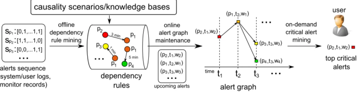
Figure 2.1: Critical alert mining: pipeline

Performance metrics. A performance metric measures an aspect of system

performance. For datacenters, common types of performance metrics include CPU and memory usage for virtual machines, error rate of disk writes for a service, or communication time between two hosts. The same type of metrics over different hosts, virtual machines, or services are considered as distinct performance metrics. In practice, system service providers e.g., LogicMonitor may cope with 2 mil-lion metrics from a datacenter with 5,000 hosts. These metrics could correlate with and cause each other due to functional or resource dependencies.

Alert and alert sequences. For a set of performance metricsP, alerts are

deter-mined by aggregating the metric values of interest. For example, in datacenters, an alert is raised when the value of a performance metric (e.g., CPU usage) goes beyond a pre-defined threshold (e.g., >75%). In this work, we define an alert as a triple u = (pu, tu, wu), where pu ∈P is a performance metric u corresponds to,

tu denotes the timestamp when the alert u happened, and wu is the weight of u,

representing the benefit ifu is fixed.

We use a sequence of alerts to characterize abnormal events for a specific performance metric. Indeed, in practice the performance metrics are typically periodically monitored to capture the abnormal events as alerts. We denote as

~sp an alert series (an ordered sequence of alerts following their timestamps), for

a specific performance metric p _∈ P. Each entry of ~sp is either 0 (normal) or 1

(alert).

To characterize causal relations between two alerts, we next introduce a notion of dependency rule. We also introduce alert graphas an intuitive graph represen-tation for multiple dependency rules.

Dependency rule. Let p and q be two distinct performance metrics. A

depen-dency rulep−→lpq qdenotes an alert issued onqat some timetis caused by an alert issued on p att′ _∈[t−l

pq, t−1], where lpq is alag fromp to q (e.g., 5 minutes).

Note that we do not specify the timet, as a dependency rule describes a statistical rule for all the observed alerts. Intuitively, a dependency rule indicates that alerts on q occurs if and only if alerts on p occurs as the cause of the alerts on q; that is, the alerts on pwill trigger the alerts on q. If certain trouble shooting action is taken to fix p, q is addressed accordingly [22, 124].

Dependency rules can be automatically learned from alert series [26, 158]. They can also be suggested by experts and existing knowledge bases [59]. To smoothen the noise or error brought by rule generation process, we associate an uncertainty to each dependency rule. In particular, we denote the uncertainty by Pr(p−→lpq q), which is the probability that the corresponding dependency rule holds.

Alert graph. An alert graph over a set of alerts V is a directed acyclic graph

G= (V, E, fe):

• Eis a set of edges inG. Letu= (pu, tu, wu) andv = (pv, tv, wv) be two alerts

in V. There is an edge (u, v) _∈ E if and only if there exists a dependency rule pu

lpupv

−−−→pv, where tu < tv, and tv −tu ≤lpq.

• feis a function that assigns for each edge (u, v) the probability thatucauses

v, i.e.,Pr(pu lpupv −−−→pv).

We shall use the following notations. Abusing the notions from tree topology, we say u (resp. v) is a parent (resp. child) of v (resp. u) if (u, v) _∈ E, and the edge (u, v) is an incoming edge of v. The topological order r of an alert u inG is defined as follows. (a) r(u) = 0 if u has no parent, and (b) r(u) = 1 + maxr(v), for all its parents v.

Following the convention of causal relation and cascading models [142], we assume that an alert is caused by a single alert issued earlier, if any. Intuitively, a path from an alert u to another alert v in the alert graph indicates a potential “causal chain” from u tov, indicated by e.g., the actual dependencies among the vulnerabilities of the servers [43].

Critical alerts. We next introduce a metric to characterize critical alerts, in

terms of how many alerts are potentially caused by them via a cascading effect (and hence are addressed if the critical ones are fixed). GivenG= (V, E, fe), a set

of fixed alertsS _⊆V, and an alertu_∈V, we use a notion ofalert-fixed probability

Pf to characterize the probability that u is fixed if S is fixed. More specifically, • Pf(S, u) = 1 if u∈S, • otherwise, Pf(S, u) = 1− Y (u′_,u)∈E 1₋Pf(S, u′)fe(u′, u) .

Based on the alert-fixed probability, we next define a set function, denoted as Gain, to characterize critical alerts. Given an alert graph G = (V, E, fe) and

S ⊆V, the gain of S is a set function

Gain(S) =X

u∈V

wu·Pf(S, u).

As remarked earlier, here wu refers to the weight of u, i.e., the benfit if u is

fixed. Intuitively, Gain(S) computes the total expected benefits induced via fixing a set of alerts S and subsequently addressing the alerts caused by S. The larger Gain(S) is, the more “critical” S is.

We next introduce the critical alert mining problem.

Definition 1. Given an alert graph G and an integerk, the critical alert mining

problem (referred to as CAM) is to find a set of k critical alerts S ⊂V such that Gain(S) is maximized.

Finding the best set of k alerts which maximize the gain is desirable albeit intractable.

Theorem 1. For a given alert graph G and an integer k, the problem CAM is

NP-complete.

Proof. We prove the NP-completeness of the decision version of CAM as follows. (1) CAM is in NP. Indeed, given an alert graph G = (V, E) and a set of vertices

S ⊆V, one can evaluateGainby computingPf(S, v) of each alertv in polynomial

time. (2) To show that CAM is NP-hard, we construct a reduction from the maximum coverage problem, which is known to be np-hard [180]. An instance

selects at most k of these sets such that the number of elements that are covered is no less than a bound B. A maximum coverage instance can be constructed as a bipartite alert graph, with each “upside” node as a set in S, each “downside” node a distinct element in these sets, and there is an edge from upside node to downside node if the corresponding element is in the set denoted by the upside node. In addition, the weights on edges are uniformly 1. Given the boundB, one may verify that there is a solution for the maximum converage problem if and only if there is a set S of k critical alerts with Gain(S) ≥ B. Therefore, CAM is at least as hard as maximum coverage problem, and is NP-hard. Hence, CAM is

np-complete.

2.3

Mining framework

In this section, we present a framework for critical alert mining. It consists of three components as illustrated in Figure 2.1: (1) offline dependency rule mining; (2) online alert graph maintenance; and (3) on-demand critical alert mining.

Offline dependency rule mining. Given a set of observed alert sequences, the

system mines the alerts of interest and their causal relations offline, and represent them as a set of dependency rules. As there are a variety of methods to model a causal relation, in this work we adopt Granger causality [26, 158], which can naturally be represented by dependency rules. An alert sequence X is said to Granger-cause another sequence Y if it can be shown, via certain statistic tests on lagged values ofX and Y, that the values ofX provide statistically significant information to predicate the future values ofY. More specifically,

(1) We collect alert sequences for all performance metrics of interest as training data, following two criteria as follows: (a) the alerts in training data should be the latest ones such that the latest dependency patterns among performance metrics can be captured; and (b) the alert information should be rich enough such that learned dependency rules would be more robust. In our work, we treat the latest one week alert data as the training data.

(2) We apply existing Granger causality analysis tools [158] to mine the depen-dency rules, and apply conditional probabilities to estimate the uncertainty of the rules [106].

The learned dependency rules are stored in knowledge bases to support on-line alert graph maintenance. Moreover, existing knowledge bases such as event causality scenarios [59], or vulnerabilities exploitation among cyber assets [43] can also be “plugged” into our critical causal mining framework. The dependency rules are then shipped to the next stage in the system to maintain alert graphs.

Online alert graph maintenance. Using dependency rules, our system

con-structs and maintains an alert graphGonline from a range of newly issued alerts. Upon an alert u from performance metric q is detected at time t, it first marks

u as a new alert in G. It then checks (1) if there exists dependency rules in the form of p_−→lpq q, and (2) whether there are alerts detected on performance metric

pduring the time period [t−lpq, t). If there exists such an alertv onp, an directed

edge from v to u is inserted, and the rule uncertainty Pr(p _−→lpq q) is associated to the edge (v, u). Following the above steps, it maintains G online for newly detected alerts.

On-demand critical alert mining. The major task (and the focus of this work) in the pipeline is to identifyk critical alerts from alert graphs. In practice, a user may specify a time window of interest, which induces an alert graph from the maintained alert graph. It contains all the alerts detected during the time window. However, the induced alert graphs can still be huge.

In this paper, we propose three algorithms to address the scalability issue: (1) a quadratic time approximation with performance guarantees on the quality of critical alerts, (2) a linear time approximation, which guarantees the alert quality for tree-structured alert graphs; and (3) sampling-based heuristics which can be tuned to balance the alert quality and response time. The critical alerts are then returned to users for further analysis and verification.

2.4

Bound and pruning algorithm

Theorem 1 tells us that it is unlikely to find a polynomial time algorithm to find the best k alerts with the maximum gain. All is not lost: we can find polynomial time algorithms that approximately identify the most critical alerts. The main result in this section is as follows.

Theorem 2. Given an alert graph G = (V, E, fe) and an integer k, (1) there

exists an algorithm inO(k_|V_||E_|)time with approximation ratio 1₋1

e, where eis

the base of natural logarithm, and (2) there exists a1−1

e approximation algorithm

in O(k|V|) time, when G is a tree.

(1) One could verify whenu _∈S1, u∈S2, or u=v,Pf(S1∪ {v}, u)−Pf(S1, u)≥

Pf(S2∪ {v}, u)−Pf(S2, u);

(2) Foru /∈S2∪ {v}, we prove the diminishing return by mathematical reduction.

(a) Assume that all u’s parents u′ _{satisfy P}

f(S1∪ {v}, u′)−Pf(S1, u′)≥Pf(S2∪ {v_}, u′_)−P

f(S2, u′).

(b) When u has only one parent, Pf(S ∪ {v}, u)−Pf(S, u) = fe(u′, u)(Pf(S ∪ {v}, u)−Pf(S, u)), and it is easy to see the diminish return for u.

(c) Assume that when u has m parents, we have a − b ≥ c −d, where a =

Q u′_∈Np(u)(1−fe(u ′_{, u)P} f(S1, u′)),b=Qu′_∈Np(u)(1−fe(u ′_{, u)P} f(S1∪ {v}, u′)),c= Q u′_∈Np(u)(1−fe(u′, u)Pf(S2, u′)), andd= Q u′_∈Np(u)(1−fe(u′, u)Pf(S2∪ {v}, u′)).

Note thatb ≥d. Consider the case when u has m+ 1 parents, andw.l.o.g., u′′ _is

the m+ 1-th parent satisfying x3−x1 ≥x4−x2, wherex3 =Pf(S1{v}, u′′),x1 =

Pf(S1, u′′),x4 =Pf(S2∪ {v}, u′′), andx2 =Pf(S2, u′′), where x1 ≤x2. Therefore,

we have a(1−x1)−b(1−x3) = a−b−ax1+bx3 = (1−x1)(a−b) + (x3−x1)b, and

c(1₋x2)−d(1−x4) = c−d−cx2+dx4 = (1−x2)(c−d)+(x4−x2)d. Thus, we obtain

a(1₋x1)−b(1−x3)≥c(1−x2)−d(1−x4), which isPf(S∪ {v}, u)−Pf(S, u) =

fe(u′, u)(Pf(S∪ {v}, u)−Pf(S, u)).

In all the cases, when u /_∈ S2 ∪ {v}, its diminishing return holds. Hence,

Gain(_·) is a submodular function. It is known that for maximizing a submodular function, a greedy strategy achieves 1− 1

e approximation ratio [139]. Theorem 2

Here e refers to Euler’s number (approximately 2.71828). Denote the optimal

k alerts as S∗_{, we present an efficient algorithm to identify k alerts S where}

Gain(S)≥(1− 1

e)Gain(S∗), in quadratic time.

We start with a greedy algorithm, denoted as Naive.

Naive greedy algorithm. Given an alert graphG= (V, E, fe) and an integerk,

Naive finds k critical alerts in k iterations as follows. (1) It initializes a set S0 to

store the selected alerts. (2) At theith iteration,Naivechecks each alert inV, and greedily picks the alert si that maximizes the incremental gain Gain(Si−1∪ {si}),

where Si−1 is the set of critical alerts found at iteration i−1. (3) It repeats the

above step until k alerts are identified. One may verify that Naive is a 1₋ 1

e approximation algorithm. To see this,

observe that the set function Gain(_·) is a monotonically submodular function. A function f(S) over a set S is called submodular if for any subset S1 ⊆ S2 ⊂ S

and x_∈ S_\S2, f(S1 ∪ {x}) - f(S1) ≥ f(S2∪ {x}) - f(S2). It is known that for

maximizing a submodular function, a greedy strategy achieves 1₋1

e approximation

ratio [139]. Hence it suffices to show that the function Gain is a monotonically submodular function. Indeed, (1) one may verify that Gain is monotonic: for any

S1 ⊆ S2 ⊆ V, Gain(S1) ≤ Gain(S2); (2) the diminishing return of Gain can be

shown by mathematical reduction.

For complexity, Naive requires k iterations, and in each iteration, it scans all the vertices u and computes Pf(Sk−1, u), which takes in total O(k|V||E|) time.

Naiveprovides a polynomial time algorithm to approximateCAMwithin 1−1 e.

Nevertheless, the scalability issue of Naivemakes it difficult to use in practice for large alert graphs. For instance, when an alert graph of around 20K vertices and

200K edges, Naive mines 6 critical alerts in more than 800 seconds. We next present a faster approximation algorithm with the same approximation ratio. By using pruning and verification, the algorithm is 30 times faster than Naive, as verified in our experimental study.

2.4.1

Pruning and verification

To select a most promising alert at each iteration, Naive evaluates the in-cremental gain for each alert in V _\S, and then selects the one of the highest incremental gain, which runs in O(|V||E|) time. Instead of blindly processing every alert, we may efficiently filter “unpromising” alerts, and then evaluate the exact gain for the remaining vertices. In particular, at each iteration i, for two alerts v′ _{and v ∈ V \S}

i−1, we compute upper bounds Uv′, Uv and lower bounds

L′

v, Lv forGain(Si−1∪ {v}) andGain(Si−1∪ {v′}) , respectively. If v′ is already not

a critical alert, all the alerts v with L′

v > Uv can be safely skipped without losing

the alert quality.

We next derive an upper and lower bound for Gain(_·), and present algorithms to compute them efficiently. Instead of visiting each alert and causal relation in

G, these algorithms compute the bounds by visiting only local information of each alert inG. This enables a fast estimation of Gain(_·).

2.4.2

Upper bound

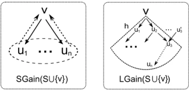
We introduce a notion ofsum gain(denoted asSGain) to characterize the upper bound for Gain(·). Given an alert graph G= (V, E, fe), an alert v ∈V, and a set

of selected critical alertsS _⊆V, an upper bound is computed asSGain(S_∪{v_}) =

P

u∈V wu·Pˆf(S∪ {v}, u), where • Pˆf(S∪ {v}, u) = 1, if u∈S;

• Pˆf(S∪ {v}, u) =P_(u′_,u)∈EPˆf(S∪ {v}, u′)fe(u′, u), if u /∈S.

The sum gainSGain(as illustrated in Figure 2.2) is an upper bound forGain(·). Better still, it can be efficiently computed.

Proposition 1. Given an alert graphG= (V, E, fe), a set of critical alertS⊆ V,

and an alert u ∈V \S, (1) Gain(S∪ {u})≤ SGain(S∪ {u}); and (2) SGain can be computed for allalerts in V in O(_|E_|) time.

We first prove Proposition 1 (1). We remark that SGain is built upon the following generalization of Bernoulli’s inequality [129]. Given xi ≤1, we have

1₋ n Y i=1 (1₋xi)≤ n X i=1 xi.

We next conduct a mathematical induction over the topological order (Sec-tion 2.2) of the alerts in G as follows.

• Consider the alerts u1 ∈ V with topological order 0: (1) if u1 ∈ S,

ˆ

Pf(S, u1) = 1 and Pf(S, u1) = 1; (2) otherwise, ˆPf(S, u1) = 0 and

• Assume that alert ui ∈ V with topological order i satisfies Pf(S, ui) ≤

ˆ

Pf(S, ui). For an alert ui+1 ∈V,

Pf(S, ui+1) = 1− Y (u′_,ui+1)∈E 1−Pf(S, u′)fe(u′, ui+1) ≤ X (u′_,ui+1)∈E Pf(S, u′)fe(u′, ui+1) ≤ X (u′_,ui+1)∈E ˆ Pf(S, u′)fe(u′, ui+1) = ˆPf(S, ui+1)

Therefore, for any u ∈ V, Pf(S, u) ≤ Pˆf(S, u). By definition, Gain(S∪ {u}) ≤

SGain(S_{∪ {}u_}). Hence, SGain is indeed an upper bound for Gain(_·).

Upper bound computation. As a constructive proof for Proposition 1 (2), we

present a procedure (denoted as computeUpperBound) for SGain to compute the upper bounds for all vertices inO(_|E_|) time.

The algorithm (not shown) follows a “bottom up” computation, starting from the alerts with the highest topological order in G. (1) It first computes the topological order for all the alerts in G. (2) Starting from the alert with the highest topological order, it computes SGain for each alert u ∈ V \S as follows: (a) SGain(S_{∪ {}u_}) =SGain(S_{∪ {}u_}) +wu, and (b) for eachu′ ∈Ni(u), it updates

SGain(S_{∪ {}u′_{}) by SGain(S∪ {u}′_{}) +f}

e(u′, u)SGain(S∪ {u}). (3) It repeats step

(2) until all the alerts are processed.

It takes O(_|E_|) time for computeUpperBound to obtain the topological order by depth-first search in step (1). Each edge in G is visited exactly once in step (2) and (3). Therefore, the algorithm runs in O(|E|) time.

LGain(S ) ∩{v} SGain(S ) ∩{v} v

u

...

u

...

Figure 2.2: AlgorithmBnP: Upper and lower bound

2.4.3

Lower bound

To compute the lower bound of Gain(_·), we introduce a notion local gain (de-noted asLGain). Given an alert graphG= (V, E), an alertv ∈V, a set of selected alerts S ⊆V, and an integer h, LGainof S∪ {v}is defined as follows.

LGain(S_{∪ {}v_}) = X

u∈Vh v

wu·Pf(S∪ {v}, u),

where h is a tunable integer, andVh

v ⊆V is a set of vertices that can be reached

from v in no more than h hops. Intuitively, LGain estimates a lower bound of Gain(S) with the impact of an alert to its local “nearby” alerts inG(as illustrated in Figure 2.2). One may verify the following.

Proposition 2. Given G= (V, E), S _⊆V, for any alertu_∈V _\S, (1)Gain(S_∪

{v_}) _≥ LGain(S _{∪ {}v_}), and (2) LGain can be computed in O(P

v∈V |Evh|) time,

where Eh

v is the set of incoming edges in G of the alerts in Vvh.

We present a procedurecomputeLowerBound to computeLGain. For each alert

v ∈V \S (e.g., u3 in Figure 2.2), the algorithm visits the alerts in Vvh and their

incoming edges (e.g., (u′

3, u3)) once, and computes LGainfollowing the definition,

in O(P

2.4.4

Algorithm BnP

Based on the upper and lower bounds, we propose an approximation, denoted asBnP. BnPenables faster critical alert mining while achieving the approximation ratio 1− 1

e. The algorithm follows Naive’s greedy strategy: given an integer

k, it conducts k iterations of search, each determines a top critical alert. The difference is that in each iteration, it invokes a procedure Prune to identify a set

C of candidate alerts for consideration.

The procedurePrune(as illustrated in Figure 2.3) invokescomputeUpperBounds and computeLowerBounds to dynamically update the lower and upper bounds for each alert by accessing their local information (lines 1-2), and filters the alerts that are not critical:

1. it scans the lower bounds LGainof each alert, and find the maximum one as

bar (line 3);

2. it scans the upper bounds SGain of each alert, and prunes those with SGain(u)< bar, adding the rest to a candidate alert set C.

Correctness and Complexity. The algorithm BnP achieves approximation

ratio 1−1

e, as it follows the same greedy strategy asNaive. Note that the pruning

procedure Prunedoes not affect the approximation ratio.

For complexity, let Cm be the maximum set of candidate sets in all the

itera-tions after pruning. For the alerts inCm, it takes BnPO(|Cm||E|) time to find a

best alert. The total time for pruning is O(k(P

u∈V |Euh|+|E|)). Hence, it takes

BnP in total O(k(P

u∈V |Euh|+|Cm||E|)) time. Moreover, |Euh| is typically small,

Input: An alert graphG= (V, E, fe);

a set of critical alertS.

Output: a set of candidate alertsC.

1. computeUpperBound (G,S); 2. computeLowerBound(G,S);

3. setbar as the largest LGainover alerts in V _\S; 4. C_{← ∅};

5. for each u_∈V _\S

6. if SGain(u)_≥bar

7. C _←C_{∪ {}u_};

8. return C;

Figure 2.3: The pruning procedure Prune

h = 1, LGain can be computed in O(dm|E|) for all the alerts, where dm is the

largest in-degree in G. Ash gets larger, the computation complexity gets higher, leading to tighter lower boundLGain. In our experimental study, by settingh= 3, 95% of the alerts are pruned, which makesBnP30 times faster thanNaivewithout losing alert quality.

Mining Alert Trees. When G is a directed tree, the algorithm BnP identifies

k critical alerts in O(k_|V_|) as follows. (1) Starting from the alerts u _∈ V of the highest topological order, it computes Gain(u) = Gain(u) +wu, and makes an

update by Gain(u′_{) = Gain(u}′_{) +f}

e(u′, u)Gain(u), if u′ is the parent of u. (2) It

alerts are processed. One iteration over (1) and (2) identifies a critical alert. (3) BnP repeats (1) and (2) to findk critical alerts.

Following the correctness analysis,BnPpreserves the approximation ratio 1−1 e

over trees. Moreover, each edge in G is visited once in a single iteration. Hence, it takesO(k|V|) time of BnP over G as trees. Theorem 2 (2) hence follows.

2.5

Tree approximation

Algorithm BnP needs to process all the candidates and their causal relations, which may not be efficient for a large amount of alert sequences. In extreme cases where few alerts are pruned, BnP degrades to its naive greedy counterpart.

As indicated by Theorem 2(2), fast approximation exists for alert graphs as trees. Following this intuition, we may make large alert graphs “small”, by spar-sifying them into directed trees, which “preserve” most of alert dependency in-formation in an alert graph. This enables both fast algorithms and low quality loss.

2.5.1

Single-tree approximation

We start by introducing a heuristic algorithmST. The basic idea is to induce amaximum directed tree (forest) T from a given alert graph G, such that for any set of alertsS in G,Gain(S) in T is “close” as much as possible to Gain(S) in G, and a fast approximation can be performed over T without much quality loss.

Maximum directed tree. Given an alert graph G = (V, E, fe), a maximum

for any u _∈ V, u has at most one incoming edge, and (2) P

hu,vi∈E′fe(u, v) is

maximized. Intuitively, T depicts a “skeleton” of an alert graph G, where causal relations always follow the most likely dependency rules.

Algorithm ST. Given an alert graph G= (V, E, fe), the single-tree

approxima-tionSTmines k critical alerts as follows. (1)STfirst finds the maximum directed tree T. To construct T, an algorithm simply selects, for each alert u in G, the incoming edge (u′_{, u) with the maximum f}

e(u′, u) among all its incoming edges.

(2) ST searches the k critical alerts following the algorithmBnP over T.

One may verify that it is in O(_|E_|) time to constructT. From Theorem 2(2), it is in O(k|V|) time to find k critical alerts in T (as either a tree or a forest). Hence, the algorithmSTtakes in totalO(_|E_|+k_|V_|) time. Note that the induced

T can be a set of disjoint trees, where the above complexity still holds.

2.5.2

Multi-tree sampling

Single-tree approximation provides fast mining method for large scale alerts. On the other hand, using induced trees to approximate causal structures may lead to biased results. For example, more dependency information could be lost for alerts with more incoming edges. To rectify this, we propose a heuristic, denoted as MTS, based on multi-tree sampling.

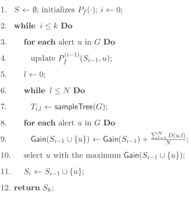
Algorithm MTS. The algorithm MTS is as illustrated in Figure 2.4. Given an

alert graph G = (V, E, fe), integer k and a sample number N, MTS starts by

initializing a set S0 as ∅, the alert-fixed probability for each node as 0 (line 1),