Generative models for group fMRI data

(1)

In Search of Functional Specificity in the Brain:

Generative Models for Group fMRI Data

by Danial Lashkari

B.S., Electrical Engineering, University of Tehran, 2004 M.S., Electrical Engineering, University of Tehran, 2005

Submitted to the Department of Electrical Engineering and Computer Science in partial fulfillment of the requirements for the degree of

Doctor of Philosophy

at the Massachusetts Institute of Technology June 2011

c

Signature of Author:

Department of Electrical Engineering and Computer Science May 19, 2011 Certified by:

Polina Golland Associate Professor of Electrical Engineering and Computer Science Thesis Co-Supervisor Certified by:

Nancy Kanwisher Ellen Swallow Richards Professor of Cognitive Neuroscience Thesis Co-Supervisor Accepted by:

Leslie A. Kolodziejski Professor of Electrical Engineering and Computer Science Chair, Committee for Graduate Students

(2)

(3)

3 In Search of Functional Specificity in the Brain:

Generative Models for Group fMRI Data by

Danial Lashkari

Submitted to the Department of Electrical Engineering and Computer Science in partial fulfillment of the requirements for the degree of

Doctor of Philosophy

Abstract

In this thesis, we develop an exploratory framework for design and analysis of fMRI studies. In our framework, the experimenter presents subjects with a broad set of stimuli/tasks relevant to the domain under study. The analysis method then auto-matically searches for likely patterns of functional specificity in the resulting data. This is in contrast to the traditional confirmatory approaches that require the experimenter to specify a narrow hypothesis a priori and aims to localize areas of the brain whose activation pattern agrees with the hypothesized response. To validate the hypothe-sis, it is usually assumed that detected areas should appear in consistent anatomical locations across subjects. Our approach relaxes the conventional anatomical consis-tency constraint to discover networks of functionally homogeneous but anatomically variable areas.

Our analysis method relies on generative models that explain fMRI data across the group as collections of brain locations with similar profiles of functional specificity. We refer to each such collection as a functional system and model it as a component of a mixture model for the data. The search for patterns of specificity corresponds to inference on the hidden variables of the model based on the observed fMRI data. We also develop a nonparametric hierarchical Bayesian model for group fMRI data that integrates the mixture model prior over activations with a model for fMRI signals.

We apply the algorithms in a study of high level vision where we consider a large space of patterns of category selectivity over 69 distinct images. The analysis success-fully discovers previously characterized face, scene, and body selective areas, among a few others, as the most dominant patterns in the data. This finding suggests that our approach can be employed to search for novel patterns of functional specificity in high level perception and cognition.

Thesis Supervisor: Polina Golland Title: Associate Professor

Thesis Supervisor: Nancy Kanwisher Title: Professor

(4)

(5)

Acknowledgements

When I arrived at MIT in September 2005, I was an aspiring physicist who could not imagine himself studying anything but quantum information science. Soon, the border-less structure of MIT exposed me to an overwhelming variety of new fascinat-ing fields. Among those was probabilistic modelfascinat-ing, to which I was introduced in the spring of 2006 through the newly designed course “Inference and Information.” As it turned out, Polina Golland, one of the two instructors, believed she could trust a novice like me with one of her research projects. The idea was to use probabilis-tic modeling techniques to help Nancy Kanwisher, a neighboring MIT neuroscientist, make more sense of her functional brain images. I knew even less about the brain and brain imaging than I did about data modeling. Yet, a sense of adventure and curiosity overcame my appreciation for the beauty of quantum mechanics and I joined Polina’s group in the computer vision lab that fall.

Over the past five years, I have often marveled at how lucky I have been to join this group. Besides all the joy I have had in exploring new subjects, having Polina as an advisor has undoubtedly been the most pleasant surprise of my MIT life. What I have earned working with Polina is by no means limited to a knowledge of generative models and statistical inference. Polina has taught me how to organize and present my ideas by her scrupulous edits on countless drafts of my writings. Polina’s conscien-tious, yet laid-back, approach to academic work, which equally emphasizes excellence and fun, has become an inspiration for all my future endeavors. I am sincerely grateful for her absolute trust, ultimate support, and unimaginable patience.

The painstaking process of working with an earnest, critical scientist from a dif-ferent discipline, Nancy, proved to be another exceptional learning experience for me. I thank Nancy for her enthusiasm and involvement and her group for their terrific help. Edward Vul and Po-Jang (Brown) Hsieh collected and preprocessed the data in the experiments reported in this thesis and also made major contributions to the development of the core ideas of the thesis through our discussions.

I would like to also thank all members of Polina’s group who coincided with me at any point during my five-year long tenure there. They sat through my many practice presentations, provided me with great feedback, and put up with my endless rambles in our reading group. Ramesh Sridharan, in particular, collaborated with me closely in 5

(6)

6

the implementation of some of the inference algorithms presented here, and kept me company in several of the many long pre-deadline nights of work. Despite my many years in the group, I never felt quite at home dealing with computing and other related issues. As a result, fellow lab-mates had to deal with my ceaseless train of computing problems and random questions. Among others, Bo Thomas Yeo, Wanmei Ou, Mert Sabuncu, Serdar Balci, Biswajit (Biz) Bose, Gerald Dalley, Jenny Yuen, Michael Sira-cusa, Archana Venkataraman, and George Chen were extremely helpful in this regard. Moreover, I also had the pleasure of collaborating with Georg Langs, Bjoern Menze, and Andrew Sweet on projects that were not reported in this thesis.

On a slightly more historical note, I am greatly indebted to the faculty who pro-vided me with support and guidance during my transition from the University of Tehran to research at MIT. In particular, I would like to express my thanks to Reza Faraji-Dana and Shamsoddin Mohajerzadeh, my advisor and my mentor at the UT, and George Verghese and Terry Orlando, from the MIT EECS department, for their tremendous assistance and advice during that process.

My experience at MIT turned out to be one of the most formative phases of my life, through which I learned much more about myself and the world around me. Weath-ering the challenges of this journey would not have been possible without the sup-port and company of many friends and allies outside the lab. Although space does not allow me to thank all of them by name, I would like to specifically acknowledge fond memories that I shared with Nabil Iqbal, Christiana Athanasiou, Maria Alejandra Menchaca Brandan, and Hila Hashemi throughout all our years together at MIT.

The work that resulted in this thesis began long before I arrived at MIT. The prepa-ration for my PhD studies may be traced back to the days when an idealist father began to enthusiastically teach his three-year old son reading and basic algebra. The academic path that brought me to MIT was meticulously engineered, years ago, by a mother’s care and attention to the early studies of her son. My father implanted in me an everlasting thirst for learning and knowing and my mother instilled in me a yearning for highest attainable levels of educational excellence. This thesis is first and foremost a tribute to my parents, to their love, and to their values, which I genuinely share and admire. I also dedicate this thesis to my sister Mitra who was very young when I left home for college studies in Tehran. Throughout my years away from home, first one thousand kilometers and then some tens of thousands, I have had far too few chances for being around her as she was growing. I hope she now accepts this dis-sertation as an ex post facto excuse for my long absence. My brother Nima, who will soon be writing his own dissertation in theoretical physics, has always been a source of pride for me. As the older brother, however, I admit that it came as a relief that I managed to obtain the first doctorate in the family, after all!

Cambridge, MA May, 2011

(7)

5 Discovering Functional Systems in High Level Vision 67 5.1 Block-Design Experiment . . . 67 5.1.1 Data . . . 67 5.1.2 Results . . . 69 Selectivity Profiles . . . 69 Spatial Maps . . . 72 5.2 Event-Related Experiment . . . 74 5.2.1 Data . . . 75 5.2.2 Results . . . 76 New Selectivities? . . . 77

Projecting the Voxels in each System Back into the Brain . . . 79

6 Nonparametric Bayesian Model for Group Functional Clustering 87 6.1 Joint Model for Group fMRI Data . . . 88

6.1.1 Model for fMRI Signals . . . 89

Priors . . . 92

6.1.2 Hierarchical Dirichlet Prior for Modeling System Variability across the Group . . . 93

6.1.3 Variational EM Inference . . . 94

(9)

CONTENTS 9

6.2.1 Preprocessing and Implementation Details . . . 97

6.2.2 Evaluation and Comparison. . . 97

6.2.3 System Functional Profiles. . . 99

6.2.4 Spatial Maps . . . 103

6.2.5 Reproducibility Analysis . . . 104

7 Conclusions 109 A Generative Models 113 A.1 Maximum Likelihood, the EM, and the Variational EM Algorithms . . . 113

A.2 Bayesian Methods . . . 114

B Derivations for Chapter 4 115 B.1 Derivations of the Update Rules. . . 115

B.2 Estimation of Concentration Parameter . . . 117

C Spatial Maps for the Event-Related Experiment in Chapter 5 119 D Derivations for Chapter 6 143 D.1 Joint Probability Distribution . . . 143

D.1.1 fMRI model . . . 143

D.1.2 Nonparametric Hierarchical Joint Model for Group fMRI Data. . 144

D.2 Minimization of the Gibbs Free Energy. . . 145

D.2.1 Auxiliary variables . . . 145

D.2.2 System memberships. . . 147

D.2.3 Voxel activation variables . . . 148

D.2.4 fMRI model variables . . . 148

D.2.5 System Activation Probabilities . . . 150

(10)

(11)

List of Figures

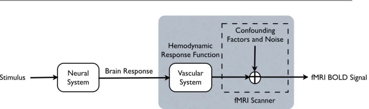
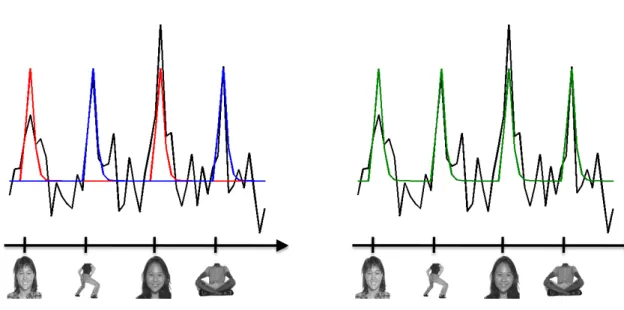
2.1 A schematic view of the relationship between the experimental protocol, the brain responses, and the BOLD measurments. The gray box indi-cates the parts of the process characterized by the linear time-invariant model of the response observed via fMRI. . . 29 2.2 The distinction between the additive model of ICA and the clustering

model. The black line indicates the hypothetical time course of a voxel; the axis shows likely onsets of a set of visual stimuli. Left, ICA may describe the black fMRI time course as a sum of the blue and red com-ponents, responsive to face and body images, respectively. However, since clustering does not allow summing different components, it may have to create a distinct component for describing the response of this voxel. We argue here that such a face-&-body selective pattern is indeed the description that we are seeking.. . . 44 4.1 An example of voxel selectivity profiles in the context of a study of

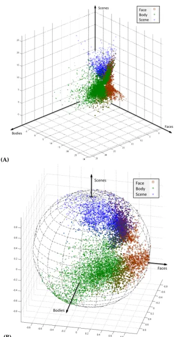
vi-sual category selectivity. The block design experiment included several categories of visual stimuli such as faces, bodies, scenes, and objects, defined as different experimental conditions. (A) Vectors of estimated brain responses ˆb= [bFaces,bBodies,bScenes]t for the voxels detected as

selec-tive to bodies, faces, and scenes in one subject. As is common in the field, the conventional method detects these voxels by performing sig-nificance tests comparing voxel’s response to the category of interest and its response to objects. (B) The corresponding selectivity profilesx

formed for the same group of voxels. . . 57

(12)

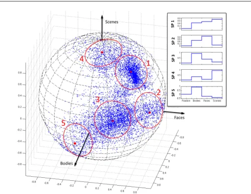
12 LIST OF FIGURES 4.2 The results of mixture model density estimation with 5 components for

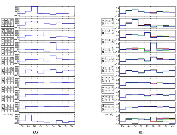
the set of selectivity profiles in Figure 4.1(B). The resulting system se-lectivity profiles (cluster centers) are denoted by the red dots; circles around them indicate the size of the corresponding clusters. The box shows an alternative presentation of the selectivity profiles where the values of their components are shown along with zero for fixation. Since this format allows presentation of the selectivity profiles in general cases withS>3, we adopt this way of illustration throughout the paper. The first selectivity profile, whose cluster includes most of the voxels in the overlapping region, does not show a differential response to our three categories of interest. Selectivity profiles 2, 3, and 4 correspond to the three original types of activation preferring faces, bodies, and scenes, respectively. Selectivity profile 5 shows exclusive selectivity for bodies along with a slightly negative response to other categories. . . 61 5.1 (A) A set of 10 discovered group system selectivity profiles for the

16-Dimensional group data. The colors (black, blue) represent the two dis-tinct components of the profiles corresponding to the same category. We added zero to each vector to represent Fixation. The weight wfor each selectivity profile is also reported along with the consistency scores (cs) and the significance values found in the permutation test, sig =

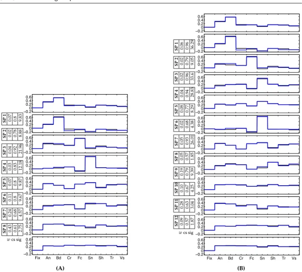
−log₁₀p. (B) A set of individual system selectivity profiles in one of the 6 subjects ordered based on matching to the group profiles in (A). . . 69 5.2 Sets of 10 discovered group system selectivity profiles for (A) 8-Dimensional,

and (B) 32-Dimensional data. Different colors (blue, black, green, red) represent different components of the profiles corresponding to the same category. We added zero to each vector to represent Fixation. The weightwfor each selectivity profile is also reported along with the con-sistency score (cs) and the significance value. . . 70 5.3 Group system selectivity profiles in the 16-Dimensional data for (A) 8,

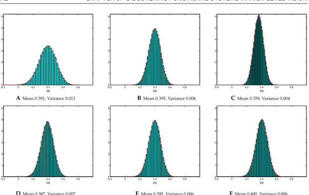
and (B) 12 clusters. The colors (blue, black) represent the two distinct components of the profiles corresponding to the same category, and the weight wfor each system is also indicated along with the consistency score (cs) and its significance value found in the permutation test. . . . 71 5.4 Null hypothesis distributions for the consistency score values, computed

from 10,000 random permutations of the data. Histograms A, B and C show the results for 8, 16, and 32-Dimensional data with 10 clusters, re-spectively. Histograms D, E, and F correspond to 8, 10, and 12 clusters in 16-Dimensional data (B and E are identical). We normalized the counts by the product of bin size and the overall number of samples so that they could be compared with the estimated Beta distribution, indicated by the dashed red line. . . 72

(13)

LIST OF FIGURES 13 5.5 Spatial maps of the face selective regions found by the significance test

(light blue) and the mixture model (red). Slices from the each map are presented in alternating rows for comparison. The approximate loca-tions of the two face-selective regions FFA and OFA are shown with yellow and purple circles, respectively. . . 73 5.6 The 69 images used in the experiment. . . 76 5.7 System profiles defined over 69 unique images. Each plot corresponds

to one identified system (of 10 total). Plots are ordered from top based on their consistency scores. Bars represent the response profile magni-tude for the group cluster, while the bars represent the 75% interquartile range of the matching individual subject clusters (see methods). ROC curves on the right show how well the system profile picks out the pre-ferred image category (defined by the image with the highest response), as evaluated on the other 68 images. As shown in text, systems 1-7 are significantly consistent across subjects, while systems 8-10 are not. . . . 78 5.8 The distribution of consistency scores in the permutation analysis, along

with the best-fitting beta-distribution, and markers indicating consis-tency scores for systems 1-10 (consisconsis-tency scores for these systems, re-spectively: 0.76, 0.73, 0.70, 0.60, 0.55, 0.51, 0.49, 0.32, 0.27, and 0.21). Because the largest consistency score in the shuffled data is 0.36, the test suggests that profiles 1-7 are significantly consistent with a p-value of 0.001. . . 79 5.9 Stimulus preference for the apparent body (a; system 1), face (b; system

2), and scene (c; system 3) systems. For each system, the set of images above the rank ordered stimulus preference shows the top 10 preferred stimuli, and the images below show the 10 least preferred stimuli. . . 80 5.10 Event-related cross-validation analysis. Half of the images were used

for mixture of functional systems (left), then the voxels corresponding to these clusters were selected as functional Regions of Interest, and the response of these regions were assessed in the held-out, independent half of the images (right).. . . 81 5.11 Clustering results on retinotopic occipital areas: Because the dominant

selective profiles found in the ventral stream do not appear when clus-tering retinotopic cortex, they must reflect higher order structure rather than low-level image properties. Profiles are ordered based on the con-sistency scores (indicated by cs in the figure). The proportional weight of each profile (the ratio of voxels assigned to the corresponding sys-tem) is indicated byw. The thick, black line shows the group profile. To present the degree of consistency of the profile across subject, we also present the individual profiles (found independently in each of the 11 subjects) that correspond to each system (thin, colored lines). . . 82

(14)

14 LIST OF FIGURES 5.12 Rank ordered image preference for system 5. The set of images above

the rank ordered stimulus preference shows the top 10 preferred stimuli, and the images below show the 10 least preferred stimuli.. . . 83 5.13 Significant systems projected back into the brain of Subject 1. As can be

seen, Systems 4, 6, and 7 arise in posterior, largely retinotopic regions. Category-selective systems 1, 2, and 3 arise in their expected locations. System 5 appears to be a functionally and anatomically intermediate region between retinotopic and category-selective cortex. For analogous maps in all subjects, see Appendix C.. . . 84 6.1 Schematic diagram illustrating the concept of a system. Systemkis

char-acterized by vector[φ_k₁,_{· · ·} ,φ_kS]t that specifies the level of activation induced in the system by each of theSstimuli. This system describes a pattern of response demonstrated by collections of voxels in all J sub-jects in the group. . . 88 6.2 Full graphical model expressing all dependencies among different

la-tent and observed variables in our model across subjects. Circles and squares indicate random variables and model parameters, respectively. Observed variables are denoted by a grey color. For a description of different variables in this figure, see Table 6.1. . . 91 6.3 System profiles of posterior probabilities of activation for each system to

different stimuli. The bar height correspond to the posterior probability of activation. . . 99 6.4 Left: system selectivity profiles estimated by the finite mixture of

func-tional systems (Lashkari et al.,2010b). The bar height corresponds to the value of components of normalized selectivity profiles. Right: profiles of independent components found by the group tensorial ICA ( Beck-mann and Smith,2005). The bar height corresponds to the value of the independent components. Both sets of profiles are defined in the space of the 69 stimuli. . . 100 6.5 Top: membership probability maps corresponding to systems 2, 9, and

12, selective respectively for bodies (magenta), scenes (yellow), and faces (cyan) in one subject. Bottom: map representing significance values −log₁₀pfor three contrasts bodies-objects (magenta), faces-objects (cyan), and scenes-objects (yellow) in the same subject. . . 101 6.6 The distributions of significance values across voxels in systems 2, 9,

and 12 for three different contrasts. For each system and each contrast, the plots report the distribution for each subject separately. The black circle indicates the mean significance value in the area; error bars corre-spond to 25th and 75th percentiles. Systems 2, 9, and 12 contain voxels with high significance values for bodies, faces, and scenes contrasts, re-spectively. . . 102

(15)

LIST OF FIGURES 15 6.7 Left: the proportion of subjects with voxels in the body-selective

sys-tem 2 at each location after nonlinear normalization to the MNI system-plate. Right: the group probability map of the body-selective

compo-nent 1 in the ICA results. . . 103

6.8 Group normalized maps for the face-selective system 9 (left), and the scene-selective system 12 (right). . . 104

6.9 Group normalized maps for system 1 (left), and system 8 (right) across all 10 subjects. . . 105

6.10 System profiles of activation probabilities found by applying the method to two independent sets of 5 subjects. The profiles were first matched across two groups using the scheme described in the text, and then matched with the system profiles found for the entire group (Figure 6.3). 106 6.11 The correlation of profiles matched between the results found on the two separate sets of subjects for the three different techniques. . . 107

B.1 Plot of functionAS(·)for different values of S. . . 118

C.1 Map of discovered systems for subject 1. . . 120

C.2 Significance map for bodies–objects contrast for subject 1. . . 120

C.3 Significance map for faces–objects contrast for subject 1.. . . 121

C.4 Significance map for scenes–objects contrast for subject 1. . . 121

(16)

16 LIST OF FIGURES

C.35 Significance map for faces–objects contrast for subject 10. . . 137

(17)

List of Tables

5.1 Asymmetric overlap measures between the spatial maps correspond-ing to our method and the conventional confirmatory approach in the block-design experiment. The exclusively selective systems for the three categories of Bodies, Faces, and Scenes, and the non-selective system (rows) are compared with the localization maps detected via traditional contrasts (columns). Values are averaged across all 6 subjects in the ex-periment. . . 75 6.1 Variables and parameters in the model. . . 90 6.2 Update rules for computing the posterior q over the unobserved

vari-ables. . . 96

(18)

(19)

Chapter 1 Introduction

U

NDERSTANDINGthe organization of human brain is one of the most ambitious projects undertaken by modern science. From basic sensorimotor tasks to abstract reasoning, all that we are capable of doing as human beings stems from the functioning of the brain. By explaining the brain, neuroscience unearths the underlying biologi-cal principles behind our perceptions, actions, emotions, motivations, and thoughts, as well as what differentiates between us in these activities. One can therefore argue that the success of brain science may have the most far-reaching and profound impli-cations among sciences in different aspects of human life. Beyond obvious medical value, scholars in disciplines as varied as education, law, business, economics, poli-tics, and philosophy have begun to actively discuss the consequences of neuroscien-tific discoveries in their respective fields. Expectedly, the staggering diversity of brain function broadens the range of the implications of neuroscience and also creates a ma-jor question for the field. How are all these different functions organized within the brain?

Functional specialization answers this question, at least in part. Many complex natural and artificial phenomena emerge in systems that comprise several interact-ing, specialized compartments. Such functional specialization is ubiquitous in many domains, particularly in biology. Bacteria are living organisms endowed with basic mechanisms of metabolism, reproduction, and even movement. In a bacterium, dif-ferent cellular regions, such as nucleoid, cytoplasm, and ribosomes, each contribute to a different aspect of the cell’s function. The same functional pigeonholing principle ex-plains different organelles in more complex cells and organs in advanced macroorganisms– including, of course, the specific functionality of the brain itself as an organ within the human body. We can provide an evolutionary justification for the emergence of spe-cialization in biological function based on an efficiency advantage. To use a metaphor, one of the hallmarks of human social evolution has been the specialization of careers, which enabled modern individuals to make more substantial progress in one specialty instead of obtaining a basic level of training in a wide variety of skills. Similarly, one can argue, once a biological unit becomes dedicated to a specific function, it can evolve to perform that task more efficiently.

Having these simple intuitions in mind, it comes as no surprise that functional specialization has been a recurring theme in neuroscience, since the inception of brain 19

(20)

20 CHAPTER 1. INTRODUCTION studies in the ninteenth century. Austrian physician and anatomist Joseph Gall (1758-1828) was one of the early pioneers of the doctrine of localization that posited that different cognitive functions were associated with different brain areas (Zola-Morgan,

1995). Gall’s theory was not based on empirical observations and was questioned soon after by the prominent French anatomist, Pierre Flourens, who concluded based on his experiments that the cerebral cortex was an indivisible unit (Changeux and Garey,

1997). For more than 150 years, generations of neuroanatomists and neuroscientists have continued the debates started with Gall and Flourens (Kanwisher,2010). Mean-while, of course, much progress has been made in our understanding of the brain. This progress, however, has been rather equivocal on the question of specificity, showing evidence both for and against it on different fronts (Schiller,1996). Most neuroscien-tists today may hold a moderate position that emphasizes understanding the extent of specificity in brain function while acknowledging its existence. Even if we agree with Gall on a fully compartmentalized picture of brain function, we still need to ex-plain the necessary subsequent integration stage in which the information processed by specialized areas is combined to create a basis for coherent human beharvior. When, where, and how such an integration happens still remains a fundamental question in neuroscience.

As the title suggests, this thesis is concerned with the question of functional speci-ficity in the brain. Broadly speaking, two important distinctions can be made in the context of the studies of functional specificity. First, we can study the brain func-tional specificity at varying spatial scales. At one end of the spectrum, we may distin-guish specificity in the function of neurons. At the other end, we may be interested in specificity at the level of large brain areas (Schiller,1996). For decades electrophysiol-ogy techniques have provided excellent means for probing functional specificity at the neuronal level (see, e.g., the groundbreaking work ofHubel and Wiesel,1962,1968). Yet studies of area-level specificity, until lately, relied primarily on patients with brain lesions. The recent advent of functional neuroimaging techniques, and in particular functional Magnetic Resonance Imaging (fMRI), revolutionized this field by offering non-invasive, large-scale observations of the brain processes in humans.

The second dimension in the study of brain specificity corresponds to specializa-tion at different levels of funcspecializa-tional abstracspecializa-tion. On one hand, we know that specific cortical patches are dedicated to the processing of low level motor and sensory inputs. The early visual cortex that includes areas V1–V5 provides a well studied example where regions with relatively distinct neuroanatomical architectures are thought to process different perceptual attributes of the visual inputs such as orientation, color, and direction of motion (Livingstone and Hubel,1995;Zeki,2005). When it comes to higher level functional specialization, for instance, high level perception or language, the current understanding of the functional organization is much less refined. Since the late nineteenth century lesion studies have suggested that the so-called Broca’s and Wernicke’s areas, in the frontal and temporal lobes of the dominant hemisphere respectively, are involved in language processing. The case of visual object recognition

(21)

Sec. 1.1. Background and Motivation 21 provides another well-studied example where category selectivity have been observed in humans and primates both at the level of neurons (Kreiman et al.,2000;Logothetis and Sheinberg,1996;Tanaka,1996) and brain areas (Kanwisher,2003,2010). Other re-ported examples of high level functional specialization include areas involved in the processing of other people’s ideas (Saxe and Kanwisher,2003;Saxe and Powell,2006), cognitively demanding tasks (Duncan,2010), as well as new language areas beyond those of Broca and Wernicke (Fedorenko et al.,2010).

This thesis develops techniques for exploratory fMRI studies of cognitive func-tional specificity. In terms of the classification described above, this problem translates into the search for the specialization in the brain at the area-level in spatial extent and high-level in abstraction. Originally, the work in this thesis was mainly meant to be a contribution to fMRI data analysis. However, the methods provided here open doors for performing novel studies that utilize the potential of our new approach to anal-ysis. Hence, the work also involves an experimental aspect related to the design of fMRI studies. Section1.1 discusses the motivations for this work in more detail and describes the particular problems addressed by methods developed in later chapters. Section1.2briefly explains the approach we have taken in this thesis for tackling those problems, enumerates its contributions, and provides an outline for the remainder of the thesis.

!

1.1 Background and Motivation

Functional MRI has played a major role in the expansion of the field of cognitive neuro-science (Gazzaniga,2004). Once fMRI allowed us to find measures of brain responses

in vivo, we were able to employ it for investigating the organization of high level

cog-nitive processes, phenomena that had hitherto been studied mainly using behavioral methods in psychology. Among domains where functional neuroimaging has made the most visible impact, vision undoubtedly stands out (Grill-Spector and Malach,

2004). In particular, fMRI studies have uncovered the properties of a number of re-gions along the ventral visual pathway that demonstrate significant selectivity for cer-tain categories of objects (Kanwisher,2003,2010). Since the studies of visual category selectivity have provided the primary motivation and the main application for the fMRI models developed in this thesis, we briefly review their findings next.

!

1.1.1 Functional Specificity and Visual Object Recognition

A ubiquitous part of our brain’s daily functions, visual object recognition has mo-tivated many neuroscientific studies in the last 50 years (Logothetis and Sheinberg,

1996). The current computational models and neuroscientific findings suggest a hier-archical processing stream in the cortex where the visual sensory input passes through different stages of representation along which the information relevant to cognitive tasks becomes more explicitly encoded (DiCarlo and Cox,2007;Riesenhuber and Pog-gio,1999;Ullman,2003). Thus, understanding the brain visual processing system

(22)

re-22 CHAPTER 1. INTRODUCTION quires the characterization of different areas of the visual cortex and their correspond-ing representations of the visual world. In the early visual areas, the representation is generally local and encodes low level features such as orientation and color. As we progress towards high level areas, the representation becomes non-local, relatively in-variant to identity-preserving transformations of the image, and predictive of image category.

Prior to the utilization of functional neuroimaging, little was known about the organization of high level visual areas in the cortex. Some studies on patients with prosopagnosia, a specific form of visual agnosia that results in impaired recognition of human faces, had suggested the existence of certain localized areas in the brain involved in face processing (Farah, 2004). Selectivity for faces had been further re-ported for neurons in the temporal cortex of primates (e.g., Desimone, 1991; Perrett et al.,1982), but that area was then believed to be generally involved in the process-ing of all complex objects (Tanaka,1996). The discovery of a small patch of cortex on the fusiform gyrus that showed larger response to face images when compared to any other objects created a breakthrough in the studies of visual object recognition ( Kan-wisher et al., 1997; McCarthy et al., 1997). This region, which was named fusiform face area (FFA), can be easily and robustly identified in fMRI experiments, making it possible to use it as a region of interest (ROI) for further characterizations (Kanwisher and Yovel,2006;Rossion et al.,2003). More recently,Tsao et al.(2006) showed that neu-rons in a homologous face selective area of primates, identified with a fMRI technique similar to the one used for humans, indeed demonstrate face selectivity.

Since the discovery of FFA, a handful of other category selective areas have been found in the extrastriate and temporal cortex. Notably, the parahippocampal place area (PPA) (Aguirre et al., 1998a;Burgess et al.,1999;Epstein and Kanwisher,1998), the extrastriate body area (EBA) (Downing et al., 2001; Peelen and Downing, 2007;

Schwarzlose et al., 2005), and the visual word form area (VWFA) (Baker et al., 2007;

Cohen et al., 2000, 2002) exhibit high selectivity for places, body parts, and ortho-graphically familiar letter strings, respectively. Selectivity for these categories have been also reported in other regions such as occipital face area (OFA) (Kanwisher and Yovel,2006) and fusiform body area (FBA) (Schwarzlose et al.,2005), as well as scene-selective regions in retrosplenial cortex (RSC) and transverse occipital sulcus (TOS) (Epstein et al.,2007).

We do not expect that the brain regions engaged in object recognition consist en-tirely of contiguous class-selective areas. In order to efficiently employ the learning capacity of the ventral visual pathway, different objects of the same class must be rep-resented by a pattern of response over some population of neurons. While the fMRI data essentially integrates the response of large populations of neurons within its spa-tial units, we can assume that the spaspa-tial patterns of fMRI response over a number of these units may still encode some information about object categories. Therefore, an alternative approach to the study of object representation attempts to find object representations distributed across large areas of cortex and overlapping across many

(23)

Sec. 1.1. Background and Motivation 23 categories of images (Cox and Savoy,2003;Hanson et al.,2004;Haxby et al.,2001,2000;

Ishai et al.,1999). Nevertheless, a vast array of studies on the category-selective areas have yielded consistent characterizations of these areas, strongly supporting the idea that some degree of category-level functional specificity is present in the visual cortex (Op de Beeck et al.,2008). The extent of this specificity is a subject of ongoing debate in the field (Kanwisher,2010). This thesis aims to contribute to our understanding of the question by providing a principled approach to search for functional specificity.

!

1.1.2 Search for Specificity Using FMRI

How can we identify a pattern of functional specificity in the brain? The category-selective areas discussed so far have been discovered in the traditional confirmatory framework1 _{for making inference from fMRI data. This approach first postulates a}

candidate pattern of functional specificity. The hypothesis may be derived from prior findings or mere intuition. Then, we design an experiment that allows us to detect brain areas that show the specificity of interest. Unfortunately, fMRI data is extremely noisy and the resulting detection map does not represent a fully faithful picture of actual brain responses. In order to confirm the hypothesis, we examine the detection maps across different subjects for contiguous areas located around the same anatom-ical landmarks. Finding such anatomanatom-ical consistency in the activated areas attests to the validity of hypothesis.

In an admirable effort to search the space of category-selectivity beyond the cur-rent findings,Downing et al.(2006) employed this confirmatory framework to test the existence of 20 different categories. Surprisingly enough, they could not confirm even a single further type of category selectivity. Yet this outcome, as well as the failure of other efforts, raises an intriguing question about functional specificity in the visual cor-tex: is there really something special about the processing of faces, scenes, and bodies, or is there something wrong with our approach to searching the space?

Although it is hard to refute the first possibility given the data at hand, there are indeed enough reasons to be suspicious about the current analysis methods. We sum-marize the main limitations of the traditional confirmatory approach as follows:

1. Manual Search of a Large Space:The space of categories that may constitute a likely

grouping of objects in the visual cortex is orders of magnitude larger than 20. A brute force search of such a large space does not appear to be a feasible strat-egy. In fact, even within the experiment performed in (Downing et al., 2006), if we consider meta-categories composed of all possible collections of their original categories, we should test for about 220 _≈₁₀6_{different candidates.}

2. Biased Characterization of Categories:We usually define categories based on

seman-tic classifications of objects. It is reasonable to expect that how the cortex groups visual stimuli for the purpose of its processing may partially reflect our concep-tual abstractions of object classes. Yet, we cannot disregard the possibility that

(24)

24 CHAPTER 1. INTRODUCTION some cortical groupings may not exactly agree with what we think of as cate-gories. In other words, we need to really search all possible selectivity patterns in the space of distinct objects, instead of confining the search to the object categories that make sense to us.

3. Unproven Assumption About the Connection Between Function and Anatomy:Is it

pos-sible that the organization of different category-selective areas varies across sub-jects in a way that does not respect the organization of anatomical landmarks? Is it possible that, instead of contiguous blob-like structures, category-selectivity appears in diffused networks of smaller regions? Current findings do not provide enough evidence for rejecting either of these possibilities. Yet, most fMRI analysis techniques still rely on the premise that functionally specific areas are constrained to be located around the same anatomical landmarks in all subjects.2

Same challenges are also present in studies of high level functional specificity beyond the visual cortex. When we get to the level of abstraction studied, say, in language, so-cial cognition, or the theory of mind, it is nevera prioriknown what types of specificity we need to consider. Moreover, our understanding of the relationship between func-tion and anatomy generally becomes looser as we progress toward the frontal lobes of the brain.

The goal of this thesis is to devise an alternative approach to the design and analy-sis of fMRI studies of functional specificity, and in particular visual category selectivity, that mitigates the aforementioned problems.

!

1.2 Contributions

In this thesis, we propose an exploratory framework for the analysis of fMRI data that enables automatic search in the space of patterns of functional specificity. We partic-ularly focus on studies of category selectivity in high level vision as a benchmark to explain and test our framework. Accordingly, we consider a visual fMRI experiment that features a number of objects or object categories to a group of subjects. Based on the estimates of brain responses from the measured fMRI signals, we defineselectivity

profilesfor different brain areas in each subject. We employ clustering to identify

func-tional systemsdefined as collections of brain locations with similar selectivity profiles

that appear consistently across subject. The methods developed here simultaneously consider all relevant brain responses to to the entire set of stimuli, and automatically learn the selectivity profiles of dominant systems from data. Crucially, our framework also avoids relying on anatomical information. Hence, they solve the most important limitations in prior studies of category selectivity discussed in the previous section.

2_{Note also that the spatial resolution of fMRI fundamentally limits the spatial extent of functional}

specificity that can be studied using this technique. The discussion here assumes that we seek likely patterns of specificity at a larger spatial scale than that of fMRI observations.

(25)

Sec. 1.3. Outline of the Thesis 25 The methods are readily applicable to other studies of cognitive functional specificity beyond vision, as we discuss throughout the thesis.

Our basic mixture model describes the distribution of the fMRI data presented in the space of selectivity profiles. The model characterizes each functional system as a mixture component. We parametrize each component of the generative model with its center and weight, which represent the mean system selectivity profile and system size, respectively. The data is directly combined across subjects irrespective of the spatial information and fitted to the same distribution. We further provide a scheme for the statistical validation of the resulting systems based on theirfunctional

consistencyacross subjects.

The method allows us to automatically search within the set of all patterns of selec-tivity implicated by the experimental paradigm. Thus, the experimental design should aim to select a representative set of stimuli that provides as much richness as possible for the corresponding search. This thesis includes two experiments that aim to charac-terize category selective areas using this scheme. The first experiment features 2 image sets from each of 8 object categories where, in the large space of many likely patterns of selectivity, the method identifies face, scene, and body selectivity as the most consis-tent ones across subject. The second experiment pushes the limits of the analysis to the space of selectivities over images of distinct objects. In the result of the analysis from this data, each system selectivity profile effectively gives an account of the grouping (categorization) of objects within that system in the visual cortex. Interestingly, even in the space of 69 distinct objects presented in this experiment, the most consistent discovered selectivity profiles correspond to categories of faces, scenes, and bodies.

Our basic method includes two separate stages: we first estimate selectivity pro-files from fMRI signals and then fit the model to the resulting data. Employing gen-erative modeling for fMRI analysis enables systematic augmentation of the basic mix-ture model to unify the two stages and to refine the assumptions of the basic mixmix-ture model. Having established the merits of our basic framework, we further develop a nonparametric hierarchical Bayesian model for group fMRI data that integrates the mixture model prior over activations with a model for fMRI signals. The nonparamet-ric aspect of the refined model allows the estimation of number of systems from the data. The hierarchical aspect of this model explicitly accounts for the variability in the sizes of systems among subjects. We derive an inference algorithm for the hierarchical Bayesian model and show the results of applying the algorithm to data from the visual fMRI study with 69 distinct stimuli. We show that the hierarchical model improves the accuracy of the basic model and the interpretability of the results while maintaining their favorable characteristics.

!

1.3 Outline of the Thesis

In the next two chapters, we provide a background for the work. Chapter 2gives a brief, general review of fMRI techniques and situates our proposed framework relative

(26)

26 CHAPTER 1. INTRODUCTION to prior work in fMRI data analysis. Chapter3reviews standard approaches to group analysis and explains the advantages of the choice made in this thesis for combining fMRI data across subjects.

Chapter4discusses the elements of our basic analysis including the basic mixture model and the consistency analysis. Chapter 5 presents the application of the basic method to data from our two visual fMRI experiments and compares them with the results of conventional confirmatory analyses.

Chapter6presents the nonparametric hierarchical Bayesian extension of the basic model and discusses the application of the corresponding inference algorithm to our visual fMRI study.

Finally, Chapter 7 discusses some avenues for the extension of this work in the future and concludes the thesis.

(27)

Chapter 2 Approaches to Inference from fMRI

Data

F

UNCTIONAL MRI yields an indirect measure of local aggregate neuronal activity based on local blood flow.1 _{The close connections between the brain metabolism}

and its activity has been known for a long time (see, e.g.Fox and Raichle,1986;Roy and Sherrington,1890). Ogawa et al. (1990) were first to develop the blood-oxygenation-level dependent (BOLD) MR contrast, which was sensitive to hemodynamic varia-tions in the Cerebral Blood Flow (CBF), and in particular to the level of deoxygenated hemoglobin in and around tissue. This development was soon followed by the ap-plication of the BOLD contrast in mapping brain activity during a task or stimulation (Bandettini et al., 1992; Kwong et al., 1992; Ogawa et al., 1992). Simultaneous elec-trophysiological recordings in monkeys have shown that BOLD signals correlate well with average, local measures of neuronal activity (Goense and Logothetis, 2008; Lo-gothetis et al.,2001;Logothetis and Wandell,2004). However, this correlation encom-passes a complex relationship between the metabolism of neuronal processes ( Mag-istretti et al.,1999) and the dynamics of the brain vascular system. The nature of this correlation is a subject of ongoing research (Attwell and Iadecola, 2002; Heeger and Ress,2002;Raichle and Mintun,2006;Schummers et al.,2008).

Throughout the past two decades, functional MRI has rapidly advanced to become one of the major tools available to neuroscientists (Logothetis,2008). Unlike positron emission tomography (PET), previously used for functional brain imaging, the BOLD contrast does not require the injection of exogenous tracers and is therefore far more suitable for neuroscience research. Compared to PET and other techniques such as Electroencephalography (EEG) and Magnetoencephalography (MEG), fMRI provides a better spatial resolution while still allowing full-brain scans. At the same time, the reliance of fMRI on the coupling between neural mechanisms and the vascular phe-nomena creates significant drawbacks for interpretation of the data (Heeger and Ress,

2002;Logothetis,2008). Moreover, the hemodynamics markedly limits the temporal

1_{Huettel et al.}₍₂₀₀₄_{) provides a detailed account of physics, physiology, and analysis of fMRI. Readers}

more interested in the underlying physics of MRI may refer to (Slichter,1990).Raichle(1998) relates the early history of functional brain imaging, which might also be of interest to some.

(28)

28 CHAPTER 2. APPROACHES TO INFERENCE FROM FMRI DATA resolution and reduces the signal to noise ratio (SNR).

We can classify the applications of fMRI into two broad categories. The first group, which mainly interests us in this thesis, involves experimental conditions associated with certain tasks or stimuli. The experimental setup for this group of studies can be devised using block or event-related design (Huettel et al.,2004). Both designs rely on averaging the BOLD signal evoked by a particular experimental condition across sev-eral trials in order to improve the signal-to-noise ratio (SNR). Block designs introduce long temporal windows presenting the same stimulus. Event-related designs rapidly present different stimuli within short periods of time, commonly in random order and with varied inter-stimulus time intervals. In addition, fMRI is extensively used in the studies of functional connectivity in the rest-state brain, which, as the name suggests, do not involve any experimental protocol (Biswal et al.,1995;Greicius et al.,2003).

An fMRI data set describes the BOLD signal in different locations in the brain vol-ume at different acquisition times during the experiment. The size ofvoxels, i.e., units of space, defines the spatial resolution of the data, commonly around 1-5 millimeters in each dimension. The temporal sampling rate in fMRI techniques is characterized by Repetition Time (TR), that is, the time interval between two subsequent data acqui-sitions, which typically ranges between 1-3 seconds. The spatiotemporal properties of the data are mainly determined by the fMRI scanner and the acquisition technique used.

Once acquired, BOLD time courses are usually first corrected for the subjects’ likely motion in the scanner. Still, the resulting data is an extremely noisy signature of the hemodynamic variations, and requires further processing in order to be informative about the brain function. In a typical protocol-based study, the analysis aims to employ our knowledge of the experimental paradigm, the spatiotemporal characteristics of fMRI, and the neuro-vascular coupling to make relevant inferences from the data. In parallel to the ongoing advances made in fMRI hardware and acquisition techniques, the methods of fMRI analysis have also continuously evolved, improving the quality of the inference or at times making new types of inference feasible (Logothetis,2008).

In this chapter, we briefly review existing methods for analysis of task-based fMRI data. Here, we restrict the discussion to inference from observations in a single subject, and postpone the discussion of group inference to the next chapter.

!

2.1 Standard Models of fMRI Data

Functional MRI data is a volumetric set of time courses; therefore, any method of anal-ysis has to include both characterizations of space and time. In this section, we discuss different approaches to modeling of these two main aspects of the data for protocol-based fMRI studies.

(29)

Sec. 2.1. Standard Models of fMRI Data 29 Neural System Vascular System Confounding Factors and Noise

Brain Response

fMRI BOLD Signal

fMRI Scanner Stimulus

Hemodynamic Response Function

Figure 2.1.A schematic view of the relationship between the experimental protocol, the brain responses, and the BOLD measurments. The gray box indicates the parts of the process characterized by the linear time-invariant model of the response observed via fMRI.

!

2.1.1 Temporal Models of fMRI Signals

Early fMRI experiments used basic block design paradigms, redolent of the then com-mon PET designs, that included two different conditions such as on/off sensory stim-ulations or left/right motor tasks (Kwong et al.,1992). Since the blocks for each con-dition were long and the involved evoked hemodynamic responses relatively strong, simple subtraction of average voxel responses in one condition from that of the other yielded clear maps of areas involved in the cognitive process (Bandettini et al.,1993). Alternatively, thresholding the correlation coefficients between voxel time courses and the protocol mitigates high levels of noise in the data (Bandettini et al.,1993). As fMRI techniques found widespread applications in neuroscientific research and studies be-gan to investigate more subtle dissociations, using, for instance, fast event-related de-signs (Dale,1999;Dale and Buckner,1997;Rosen et al.,1998;Zarahn et al.,1997a), the need for a more accurate temporal characterization of data became evident.

Linear Temporal Model of fMRI Response

Despite the complexity of the underlying physiology and physics of fMRI,Boynton et al.(1996) provided evidence that we can approximately model the relationship be-tween behavioral stimulation and measured BOLD signals by a linear time-invariant (LTI) system. Such linear models, which also justify the correlation analyses, have proved exceptionally successful in practice (Buxton et al., 2004; Cohen,1997;Friston et al.,1994). The linear temporal model assumes that the fMRI response results from additive contributions of stimuli,2 _{confound factors, and noise, and that the fMRI}

re-sponse to a stimulus is fixed, irrespective of the stimulus onset and its duration. Fig-ure2.1presents a schematic view of the model. We present a stimulus during the ex-periment and aim to find the brain response. Neural mechanisms commonly studied

2_{In this section, I interchangeably use the terms}_stimulus_and_{experimental condition}_{, by which I mean}

(30)

30 CHAPTER 2. APPROACHES TO INFERENCE FROM FMRI DATA in fMRI experiments have a response time scale on the order of at most few hundred milliseconds, while typical TRs in fMRI are 1-3 seconds. We assume that the neural system, the first block in the figure, does not introduce any delay to the signal, relative to the temporal dynamics of the data. The brain response is then convolved with the hemodynamic response function (HRF), a function that peaks at about 6-9 seconds and models the intrinsic delay observed between the stimulus and the measured BOLD sig-nal (Bandettini et al.,1993). Finally, the model assumes that a number of confounds, such as a commonly observed linear magnetic drift term (Friston et al.,1995c), is added to the signal prior to observation, along with Gaussian signal noise. The fMRI signal of any voxel during the experiment includes not only a delayed contribution from brain responses to all previous stimuli but also contributions from several such confound factors.

Leti ∈ V indicate a voxel within the setV ofVvoxels imaged in the fMRI study. In an experiment with a setS of Sdifferent experimental conditions, we letΩ_s(t)be

a binary indicator function that shows whether stimuluss _{∈ S} is present during the experiment at timet. The model implies that the hemodynamic response of voxeliat timetis of the form:

bis Ωs∗τ(t), (2.1)

where bis denotes the voxel’s response to stimulus s , τ(t) is the hemodynamic

re-sponse function, and∗indicates convolution. If we define Gst = Ωs∗τ(t)to be the

hemodynamic response to stimulussat timet, we form the fMRI responseyitof voxeli

as:

yit=

∑

s Gstbis+

∑

h

Fdteid+#it, 1≤t≤ T (2.2)

whereTis the number of points in the time course,Fdtrepresents nuisance factordat

timet, and#_itis the Gaussian noise term. Stacking up the variables as vectors, we can

rewrite (2.2) in the matrix form, as

yi = Gbi+Fei+!i. (2.3)

Vectorb_i _∈ IRSdescribes the response of locationiin the brain to all different stimuli

presented in the experiment. For now, we ignore the spatial dependencies among the variables, and consider equation (2.2) independently for each voxel. If we further assume that the Gaussian noise is white, i.e.,!_i i._∼i.d.Normal(0,λ_i−1I), we can estimate b_i using a simple least squares regression:3

[bˆ_iteˆt_i] =yt_iA(AtA)−1, (2.4)

where we have defined thedesign matrixA = [G F], andAt _{denotes the transpose of}

matrixA. The estimation procedure is the same for block design and event-related

3_{Of course, the derivation is possible only as long as matrix}_A_{remains nonsingular, a condition that}

(31)

Sec. 2.1. Standard Models of fMRI Data 31 experiments since as far as the model is concerned all differences between protocols are contained within functionsIs(t).

The above treatment assumes a known, a priori given HRF.Boynton et al.(1996) suggested a two parameter gamma function as an empirical approximation for the HRF, characterized by a time constant and a phase delay, and shifted by an overall temporal delay. Aguirre et al. (1998b) further demonstrated evidence for relative ro-bustness of the estimated HRF across experimental sessions for the same subjects, but suggested that variability across subjects may be considerable. To address the variabil-ity concerns, several methods have been proposed for simultaneous estimation of the HRF and brain responses. One approach is to estimate the HRF as a linear combination of basis functions, e.g., Fourier basis functions (Josephs et al.,1997) or gamma func-tions and their derivatives (Friston et al.,1998a). More recent models employ Bayesian techniques for the estimation of HRF from data (Ciuciu et al.,2003; Genovese, 2000;

G¨ossl et al.,2001b;Makni et al.,2005;Marrelec et al.,2003;Woolrich et al.,2004b). Equation (2.4) makes a simplifying assumption that the temporal components of noise are independent of each other. In reality however, unwanted physiological and physical contributions in the signal exhibit non-zero temporal autocorrelations ( Fris-ton et al., 1994). Aguirre et al.(1997) andZarahn et al. (1997b) empirically demon-strated that the power spectrum of the noise can be characterized by the inverse of frequency, and therefore does not comply with a white noise model. Bullmore et al.

(1996) suggested using a first order autoregressive model AR(1) instead to directly model noise autocorrelations. Purdon and Weisskoff(1998) further modified this AR model by adding to it a white noise component.

Some methods handle the autocorrelations prior to the main linear modeling as a preprocessing step. For instance,coloringmay be used by further temporal smoothing of the signal to the point that the original autocorrelations are overwhelmed and can be ignored (Friston et al.,1995b,2000a;Worsley and Friston,1995). Alternatively,

pre-whitening first estimates noise autocorrelations and uses the estimates to whiten the

noise (Bullmore et al.,2001;Burock and Dale,2000;Woolrich et al.,2001). Similar to the estimation of the HRF, Bayesian methods can also be used here to jointly estimate the brain response and noise characteristics (Friston et al.,2002a). Indeed, many recent analysis techniques take this approach in conjunction with AR models (see, e.g.,Makni et al.,2008;Penny et al.,2005;Woolrich et al.,2004c).

Other Models

As already mentioned, the standard linear model of fMRI signal comes with well-known limitations. Deviations from linearity are observed especially when stimuli are not well separated (Glover, 1999). Friston et al. (1998b) suggested using a Volterra series expansion of a nonlinear response kernel to account for such nonlinearities in the response. Physiologically-informed models such as the so-calledballoon model at-tempt to explain the nonlinear dynamics of BOLD signals using the specifics of the neuro-vascular coupling in terms of relevant vascular variables such as cerebral blood

(32)

32 CHAPTER 2. APPROACHES TO INFERENCE FROM FMRI DATA volume (CBV) and cerebral metabolic rate of oxygen (CMRO2) (Buxton et al., 2004,

1998;Friston et al.,2000b).

!

2.1.2 Spatial Models of fMRI Signals

Since the very early days, much of the excitement about fMRI has been commonly as-cribed to its potential forlocalizationof different functions in the brain (e.g.,Cohen and Bookheimer,1994). In the same way that structural MRI earlier provided us within vivomaps of brain anatomy, fMRI now enables us to catch a glimpse of maps of brain function, or so the argument goes. The presence of the temporal dimension in fMRI allows us to change an experimental variable and observe how different brain loca-tions respond to that change. If we observe a large response in any location (voxel), we declare that brain area active. In reality, the actual picture of functional organiza-tion in the brain may be more complex and involve interacorganiza-tions that evoke responses based on the context, prior stimulation, etc. Nevertheless, considering the rudimen-tary stages of our knowledge about the brain function, the localization picture can still help us gain important insights. The localization view has had great success in popu-larizing fMRI research through its renderings of intuitive maps of brain activation. The detection of active areas through statistical tests and their visualization as correspond-ing activation maps form the core of the traditional confirmatory (hypothesis-driven) analysis, which we will discuss in more detail in Section2.2. The majority of fMRI analysis techniques have been developed with the aim of improving the quality of activation maps, as the end result of the analysis.

Smoothing of Spatial Maps

In its most basic format, the detection of activated areas is performed through amass

univariateanalysis that tests the response of each voxel separately (Friston et al.,1994).

In the temporal model discussed in Section2.1.1, this basic approach corresponds to the assumption of independence among voxels. The analysis is simple, fast, and is widely used in practice. Yet if applied to raw time courses, the method usually creates grainy maps due to the excessive levels of noise. To further mitigate the noise and create maps that agree with our intuition about the contiguity of activated areas, it is common to apply spatial Gaussian smoothing to the data prior to analysis. Depend-ing on the noise properties of the scanner and data, Gaussian filters with full width at half maximum (FWHM) of 3-9mm are typically used, the larger filters being more suited to data with lower SNR. Ideally, the filter size should closely match the size of activated regions we are seeking (Worsley et al.,1996a). Obviously, we do not always have gooda priori estimates of the size of activations. As a result, although common in practice, the application of isotropic Gaussian filters may in fact cause blurring of the data and loss of fine spatial information. Alternative spatial denoising schemes in-clude wavelet-based methods (Wink and Roerdink,2004) or nonlinear smoothing that preserves edges (Smith and Brady,1997). Other methods account for the structure of

(33)

Sec. 2.1. Standard Models of fMRI Data 33 cortical surface in the smoothing of images (Andrade et al.,2001), or explicitly project the data onto the flattened map of the cortical surface before smoothing (Fischl et al.,

1999).

Instead of smoothing the data as a preprocessing step, spatiotemporal analysis schemes explicitly encode spatial contiguity assumptions in their models of fMRI time courses. A simple approach is that ofKatanoda et al.(2002) who include the neighbor-ing time courses in the estimation of brain response of each voxel. In the system iden-tification setting, Purdon et al. (2001) andSolo et al. (2001) estimate brain responses by adding a spatial regularization term to their model. From the Bayesian perspec-tive, such a regularization corresponds to a prior distribution on brain responses that encourages contiguity (G¨ossl et al.,2001a). This approach is further extended to also include spatial priors for the parameters of the autoregressive noise model in (Penny et al., 2005), as well as the estimation of HRF in (Woolrich et al., 2004c). In earlier work,Descombes et al.(1998) suggested applying 4-dimensional continuous Markov random fields (MRF) in both space and time for a Bayesian restoration of brain re-sponses.

Discrete Activation Models

Instead of smoothing the data or the brain responses, MRFs can be alternatively used in a discrete setting to encourage contiguity in the final maps of activated areas ( Cos-man et al.,2004;Kim et al.,2000;Ou and Golland,2005;Ou et al.,2010;Svens´en et al.,

2002b). Conceptually, the method is also closely related to the mixture model detec-tion (Everitt and Bullmore,1999;Makni et al.,2005) in that both approaches explicitly define binary latent activation variablesxto explain voxel brain responses. The

dis-tribution of observed fMRI signals yin each voxel (or some other statistics that is a

function ofy) is described while conditioning onx, which indicates whether or not the

voxel is activated by a particular stimulus. By adding the discrete MRF as a prior on the distribution of activation variables over the image, we penalize neighboring voxels with mismatched activation labels in the resulting activation map (Cosman et al.,2004;

Rajapakse and Piyaratna,2001;Salli et al.,2002). Since the observed data does not get artificially blurred, the method may be more sensitive in detecting the edges of acti-vated areas (Salli et al.,2001). As another example,Hartvig and Jensen(2000) employ a similar mixture model but describe the signal statistics in each voxel only in terms of its direct neighbors, independently of the rest of the image. Woolrich et al.(2005) add a third label representing de-activation, and further provide a method for estimating the discrete MRF parameter that controls the amount of spatial regularization.

Parcel-based Models of Spatial Maps

While encouraging contiguity, the methods described so far do not actually provide any model for the spatial configurations of activation areas. Simple modeling of such configurations can be achieved using extensions of mixture models. Penny and