Studies of Light-Matter Interactions in Atomic Ensembles for Creation of Entangled States and Quantum Interfaces

(1)

Studies of Light-Matter Interactions in Atomic

Ensembles for Creation of Entangled States and

Quantum Interfaces

by

Tanvi P. Gujarati

A dissertation submitted in partial fulfillment of the requirements for the degree of

Doctor of Philosophy (Physics)

in The University of Michigan 2019

Doctoral Committee:

Professor Luming Duan, Co-Chair Professor Alex Kuzmich, Co-Chair Associate Professor Hui Deng Professor Georg Raithel

(2)

(3)

Tanvi Gujarati

[email protected]

ORCID ID: 0000-0002-8463-3037

c

(4)

(5)

ACKNOWLEDGEMENTS

Time is a mysterious thing, it knows how to fly fast but has never learned to stand still. All I hope is that it slows down for only a few moments so that I can deeply thank everyone who helped me reach here.

It was the time to apply to universities for PhD positions, and I remember dis-cussing this with one of my undergrad teachers, Prof. Anil Shaji. He had asked me if there was a particular field that I felt strongly about for pursuing research and I had told him that I wasn’t sure, but I found light fascinating and wanted to learn more about light-matter interactions. Fast forward, I was fortunate to be a part of Prof. Luming Duan’s research group where I could shine light upon, well, light.

I am immensely thankful to Prof. Luming for his guidance throughout the years of my PhD program. It has been a great learning experience to have worked with him. I hope and wish that consciously or unconsciously I have been able to imbibe some of his many virtuous qualities like his calm demeanor, humility and sharp intellect. Thank you for giving me an opportunity to learn from you and also for the chance to travel to China! My PhD experience wouldn’t have been the same if it wasn’t for my fellow lab mates. I am grateful to Zhen Zhang, Dong-Ling Deng, Sheng-Tao Wang, Zhengyu Zhang, Yukai Wu and Ceren Dag for helping me learn and understand many different concepts and topics, not only about science, but also about cultures, languages and food! It has been an honour to have known such hard working and amazing people. I would also like to thank Prof. Paul Berman, Prof. Alex Kuzmich, Prof. Georg Raithel, Prof. Kai Sun, Prof. Emanuel Gull and Prof. Wolfgang Lorenzon for their

(6)

valuable support and guidance. I am also grateful to Prof. John Schotland and Prof. Hui Deng for being a part of my thesis committee. I will be forever grateful to Prof. Anil Shaji, Prof. Shaijumon, Prof. Sreedhar Dutta, Prof. S. Shankarnaryanan, Prof. Archana Pai, Prof. Hema Somanathan, Prof. E.D. Jemmis, Prof. Gopinanthan and all my teachers at IISER-TVM for shaping my curiosity and encouraging me always. A special thanks to my friends Jamie McLennan and Uttam Paudel for the wonderful and eye opening discussions.

When someone asks if moving to a new country, away from your family and friends is very difficult, it makes me wonder how has it affected me? It would have been very difficult had it not been for all the fabulous people I got to meet and share my happiness and PhD pains with. Transition to Ann Arbor couldn’t have been smoother all because of Surojit, Vimal, Dhruv and Kelly. Every experience that we have had, will always be cherished. A heartfelt thank you to Neha, Mohit N., Subhashis, Animesh, Siva, Manu, Mantha, Naincy, Prachi, Adithya and all the wonderful friends for all the memorable times we have spent together! Neha and Mohit N., chai-pe-charcha always woke me up! They say friends that you make in your college years are for life, and that couldn’t be more true. Thank you dearest Saranya, Manogna, Pranav, Varma, Gaurav, Gopu, Pooja, Preeti and the whole IISER-TVM gang for being my rock solid support. Thank you Atmaram and Kashi for bringing more love and wisdom in my life. You are all a part of my family now.

And finally, family. I am the luckiest person in the world to have a family like ours and even this is an understatement. Thank you so much Dadi, Dada, Pappa and Mummy, Pappa and Mummy again, Madhavi, Saurabh, Prateek, Pooja, Bharati Masi and Masaji and most of all Ved! I have no words to describe how much your love and support means to me and getting here wouldn’t have been possible without you all. There are so many more people that I want to thank and remember, I hope my gratitude reaches you, thank you all! And finally, my dearest husband and partner

(7)

in all my dreams for a great future, thank you from the bottom of my heart. Thank you, Mohit J., thank you for being there for me since kindergarten!

(8)

LIST OF FIGURES

1.1 Schematic of a Quantum Network . . . 12 2.1 Λ atomic level structure . . . 18 2.2 Schematic of Rydberg blockade . . . 21 2.3 Atomic level structure and pulse scheme for GHZ state generation . 23 2.4 Population distribution of the control atom for different values of

detuning and Rabi frequencies . . . 26 2.5 Population distribution of ensemble atoms in the multi-particle ground

states |gN_i _and _|_sN_i _{. . . .} ₃₀

2.6 Effect of spontaneous emissions on ensemble atoms . . . 36 2.7 Implementation of the GHZ state generation protocol for N=5 . . . 37 2.8 Fidelity of the final state with respect to the state |gNi√+|sNi

2 . . . 38

2.9 Fidelity of the final state with respect to |gNi√+|sNi

2 with spontaneous

emissions . . . 39 3.1 Working of quantum repeaters . . . 42 3.2 Entanglement generation between two neighboring atomic ensembles 45 3.3 Entanglement swapping between two neighbouring entangled segments 45 3.4 Atomic level diagram for the DLCZ protocol . . . 49 3.5 Experimental configuration of the write-read process . . . 72 3.6 Intrinsic retrieval efficiency as a function of width ratio . . . 75

(12)

3.7 Intrinsic retrieval efficiency as a function of optical depth for skew angle Θ = 0o _{. . . .} ₇₅

3.8 Intrinsic retrieval efficiency as a function of optical depth for skew angle Θ = 2o _{. . . .} ₇₆

3.9 Intrinsic retrieval efficiency as a function of memory storage time . . 76 3.10 The normalized angular mode function of the idler photon for storage

time Tm = 0µs and skew angle Θ = 0o . . . 78

3.11 The normalized angular mode function of the idler photon for storage time Tm = 100µs and skew angle Θ = 1o . . . 79

3.12 The normalized angular mode function of the idler photon for storage time Tm = 200µs and skew angle Θ = 2o . . . 80

(13)

LIST OF APPENDICES

Appendix

A. Derivation of the Eigenvalue Structure . . . 87

(14)

LIST OF ABBREVIATIONS

DLCZ Duan-Lukin-Cirac-Zoller

EIT Electromagnetically Induced Transparency

EPR Einstein-Podolsky-Rosen

GHZ Greenberger-Horne-Zeilinger

IRE Intrinsic Retrieval Efficiency

OD Optical Depth

RWA Rotating Wave Approximation

STIRAP Stimulated Raman Adiabatic Passage

(15)

ABSTRACT

The field of quantum computation and communication has prospered over the last few decades because of multiple advances in our understanding of trapping and controlling physical quantum systems like neutral atoms, superconducting qubits, trapped ions, quantum dots etc. using light. A lot of research has gone into develop-ment of techniques which facilitate trapping and manipulation of ensembles of neutral atoms by studying how the atomic properties of the system respond to properties of light used to control them. In this dissertation we shall explore some applications of light-matter interactions in ensembles of lambda three level neutral atoms for the purpose of entanglement generation and distribution.

The first part of this dissertation focuses on the study of a protocol that can be used to generate multi-particle entangled quantum states called the Greenberger-Horne-Zeilinger (GHZ) states in an ensemble of N neutral atoms. Schemes for creation of N particle entangled Greenberger-Horne-Zeilinger (GHZ) states are important for understanding multi-particle non-classical correlations. A theoretical protocol for creation of a multi-particle GHZ state implemented on a target ensemble of N, three-level Rydberg atoms and a single Rydberg atom as a control using Stimulated Raman Adiabatic Passage (STIRAP) is presented. We work in the Rydberg blockade regime for the ensemble atoms induced due to excitation of the control atom to a high lying Rydberg level. It is shown that using STIRAP, atoms from one ground state of the ensemble can be adiabatically transferred with high fidelity to the other multi-particle ground state, depending on the state of the control atom. Measurement of the control atom in a specific basis after this conditional transfer facilitates one-step creation of

(16)

a N particle GHZ state. A thorough analysis of adiabatic conditions associated with STIRAP for this scheme and the influence of radiative decay from the excited Rydberg levels is presented. The most important and novel feature of this scheme is that it is immune to the decay rate of the excited level in ensemble atoms and provides a robust way of creating GHZ states.

In the second part of this dissertation, we study atomic ensemble based quan-tum interfaces used in quanquan-tum repeater protocols for entanglement distribution. Quantum interfaces provide a platform where in the flying photonic qubits used for information and entanglement transfer can interact with a physical system which stores, processes and releases this information back as photons. The Duan-Lukin-Cirac-Zoller (DLCZ) quantum repeater protocol, which was proposed to realize long distance quantum communication, requires usage of quantum memories or quantum interfaces. Atomic ensembles interacting with optical beams based on off-resonant Raman scattering serve as convenient on-demand quantum memories. Here a com-plete, free space, three-dimensional theory of the associated read and write process for this quantum memory is worked out with the aim of understanding intrinsic retrieval efficiency. We develop a formalism to calculate the transverse mode structure for the signal and the idler photons and use the formalism to study the intrinsic retrieval efficiency under various configurations. The effects of atomic density fluctuations and atomic motion are incorporated by numerically simulating this system for a range of realistic experimental parameters. Results describe the variation in the intrinsic retrieval efficiency as a function of the memory storage time for skewed beam config-uration at a finite temperature, which provides valuable information for optimization of the retrieval efficiency in experiments.

(17)

CHAPTER I

Introduction

1.1 Motivation

“The changing of Bodies into Light, and Light into Bodies, is very conformable to the Course of Nature, which seems delighted with Transmutations. ”

-Sir Isaac Newton Opticks, 2nd edition (1718), Book 3, Query 30, 349.

What we see and what we don’t, is a matter of how light interacts with matter. Whether it’s the light being emitted from the sun, or that which bounces off the sur-face of water or even that which is absorbed by the rods in the retina (quantum or not [1]) are all instances of light interacting with matter. Quantum mechanical theories have succeeded immensely in describing the structure of matter [2–5]. The natural question then arises, whether light can also be described quantum mechanically and when is it that such a description is necessary? The field of quantum optics with it’s rich history provides answers to these questions with the perspective of how light interacts with matter.

Towards the end of the 19thcentury - beginning of 20th, new understanding regard-ing the nature of radiation started unfoldregard-ing when Max Planck modelled the black body radiations using discrete quanta of light [6] soon to be followed by Einstein’s

(18)

description of the photo-electric effect [7]. What started out as spectroscopic studies of atomic level structure [5, 8] paved way for lasers [9–11], complex descriptions of non-classical states of light on interaction with matter [12–14], trapping and cooling matter to study exotic phenomena like BECs [15–17] and Rydberg molecules [18]. In the past few decades, with the amalgamation of the two fields of quantum optics and computer science, a lot of path breaking research and innovation in the field of quan-tum information has been achieved. The understanding that quanquan-tum entanglement can be looked upon as a resource has led to development of many quantum com-munication protocols like quantum teleportation [19–21] and quantum cryptography [22, 23] to name a few. The fact that we now have functional quantum computers based on varied platforms ranging from atomic scale systems like ions and neutral atoms to macroscopic systems with superconducting qubits has been made possible due to theoretical and experimental progress in the understanding of light-matter interactions.

In this dissertation we are going to explore two different phenomenon that arise due to light-matter interactions in atomic ensembles using tools from quantum op-tics. We will study a protocol to generate highly entangled quantum states called the Greenberger-Horne-Zeilinger (GHZ) states using atomic ensembles in the first half. Then, using similar atomic ensembles but a different flavour of light-matter interactions, we will study the efficiency of atomic interfaces used for quantum com-munication protocols. Before we start delving into the details of these two systems, let us review the concepts that will be relevant for the forthcoming discussions.

1.2 Background

In this section, we will briefly discuss the Hamiltonians used for treating light-matter interactions using an example of a two-level atom. We will then focus on the differences between systems with multiple atoms in ensembles interacting with

(19)

light as opposed to single atom systems followed by a short discussion on quantum communication and quantum networks.

1.2.1 Light-matter interactions

Let us start by describing the method that is used in this dissertation to model light-matter interactions in quantum atomic systems. There are two major ap-proaches that are used to describe matter interacting with light, the semi-classical approach and the quantum optics approach. In the semi-classical approach, matter is modelled quantum mechanically and light is described classically, whereas in the quantum approach both light and matter are described quantum mechanically. The choice of using one method or the other depends on the phenomenon that one wishes to describe. A general rule of thumb is to use a quantized description of electric field when the average number of photons in the system under consideration is of the order or less compared to the number of atoms in the system [24]. Let us first look at the Hamiltonian that describes light-matter interactions semi-classically followed by the quantum optical treatment.

Consider a mono-chromatic classical electric field given in Eq. (1.2) with frequency

ω, wave-vectorkand unit polarization vectorε at a point r. Such a mono-chromatic field is typically used to describe electric field generated from lasers which are generally used for manipulating atoms.

E(r, t) = E0εcos(ωt−k·r) (1.1) = E0ε 2 (e −i(ωt−k·r) +ei(ωt−k·r)) (1.2) ≡ E+(r, t) +E−(r, t) (1.3)

For the kind of interactions that we will be interested in, the wavelength of the light used is much longer than the size of atom, which means that the electric field is

(20)

constant over the extent of the atom and it is given by the value of the field evaluated at the nucleus of the atom. This is called the dipole approximation or the long-wavelength approximation [25]. Consider a two-level atom with a ground state level |gi and an exited level |ei stationary at position r. Here we are approximating an atom that has an infinite set of bound levels by two levels under the assumption that the light interacting with this atom does not excite any other atomic levels. Let the energy of the state |gi be given by Eg and that of the excited state be Ee. We can

set the ground state energy to be 0 so that the energy of the excited state on the relative scale is now given by E =_~ω0 =Ee−Eg. The Hamiltonian for this system,

H, is the sum of the Hamiltonian for free atom, HA, and the atom-field interaction

Hamiltonian in the dipole approximation, HAF.

ˆ H = HˆA+ ˆHAF (1.4) ˆ HA = ~ω0|eihe| (1.5) ˆ HAF = −µˆ·E(r, t) (1.6)

In the above Eq. (1.6), ˆµ=−eˆre is the dipole moment of the atom with ˆre being the

position operator of the electron in the atom relative to the nucleus ande= 1.6∗10−19

C is the electron charge. Since the atomic operator ˆrehas an odd parity and the atom

has an inversion symmetry, the diagonal elements corresponding to the dipole moment operator vanish [24, 25]. Thus, we can expand the dipole moment operator as in Eq. (1.7):

ˆ

µ = hg|µˆ|ei|gihe|+he|µˆ|gi|eihg| (1.7)

≡ µˆ++ ˆµ− (1.8)

(21)

value of |gihe| for any state under free atom Hamiltonian evolution goes as e−iω0t_.

Thus, ˆµ±∝e∓iω0t_{. On expanding the interaction part of the Hamiltonian using Eqs.}

(1.3),(1.6) and (1.8) we get:

ˆ

HAF = −( ˆµ++ ˆµ−)·(E+(r, t) +E−(r, t)) (1.9)

The terms in Eq. (1.9), ˆµ± ·E±(r, t) ∝ e∓i(ω0+ω)t _{and the other two terms go as,}

ˆ

µ± ·E∓(r, t) ∝ e∓i(ω0−ω)t_{. Let us define the detuning as} _δ ₌ _ω

0 − ω. Assuming

that ω0 +ω |δ| we keep only the terms with slow dynamics corresponding to

the frequency δ. The terms oscillating with the frequency |ω0+ω| will be averaged

over and washed out on the time scales of δ−1. This is called the Rotating Wave Approximation (RWA) [5, 24, 25]. Let us also define:

Ω0 =

hg|µˆ·ε|eiE0

~

(1.10)

as the Rabi frequency of the light-matter interaction. Rabi frequency is a measure of how strongly given light and matter interact with each other. We can now rewrite the full Hamiltonian of the system as:

Eq. (1.11) is a thoroughly studied form of the Hamiltonian for light-matter interac-tions that gives rise to many phenomena like Rabi flopping, Ramsey Fringes, Spin echoes, Mollow Triplet spectrum to name a few [5, 24–26]. Modifications to this Hamiltonian can be introduced by adding more atomic levels as well as electric fields with more than one frequency components. Let us now extend this analysis to the case when electric field is treated quantum mechanically.

(22)

only a few photons like spontaneous emissions, fields in a cavity etc. We shall not elaborate on the methods used for quantization of electric fields here, more informa-tion on that can be found in [27, 28]. The general way of quantizainforma-tion is to assign annihilation and creation operators to classical spatial field modes associated with a set of given boundary conditions.

Consider a cubic volume V of free space with the dimension of each side given by

L. The classical field modes with these boundary conditions are given by plane wave eigen-modes eik·r, where: k = kxx+kyy+kzz (1.12) kx = 2πnx L , ky = 2πny L and kz = 2πnz L (1.13)

nx, ny and nz are integers. The expression for quantized electric field in free space of

volumeV is given in Eq. (1.14) [24]

ˆ E(r) = iX j Ej[âjεjeikj·r−â † jε ∗ je −ikj·r_] _(1.14) ≡ Eˆ+(r) + Ê−(r) (1.15)

In the above equation,krepresents the wave-vector andεthe polarization unit vector. For electric fields in free space, kj ·εj = 0. The sum is taken over all field modes

which include two independent polarization directions for a given frequency mode. Operators ˆaj and ˆa

†

j are the annihilation and creation operators for each mode j

respectively. They satisfy the commutation relations given in Eq. (1.16)-(1.17)

[âi,âj] = [â † i,aˆ † j] = 0 (1.16) [âi,aˆ†j] =δij (1.17)

(23)

In Eq. (1.14),Ej is the real electric field co-efficient and by choosing it to be: Ej = s ~|kj|c 20V (1.18)

we can write the free field Hamiltonian as given in Eq. (1.19)

ˆ HF = X j ~ωj(ˆa † jaˆj+ 1 2) (1.19)

where ωj = |kj|c is the angular frequency of the electric field mode j and c is the

speed of light in vacuum. Also, in Eq. (1.18)0is the permittivity of free space. From

the Hamiltonian in Eq. (1.19), we notice that quantized electric field in free space is analogous to a sum of harmonic oscillators each operating at a different frequency which can be determined by the eigen-modes of plane waves in a cubic volumeV. The constant factor of 1₂ P

j~ωj leads to divergences when calculating the energy density

of vacuum field. This can be taken care of by renormalization techniques [29]. For our purpose we shall ignore the contributions from this zero-point energy.

The choice of the quantization volume V is arbitrary, one can choose volumes of different shapes and sizes but the real measurable physical quantities should remain independent of them. The final step in quantization is to take the limit L→ ∞such that V would include all space. When taking the limit to infinity, following the rules laid out below in Eqs. (1.20) and (1.21) will make calculations easier and help in accounting for extra factors of V.

X k → V (2π)3 ∞ Z −∞ dkx ∞ Z −∞ dky ∞ Z −∞ dkz (1.20)

(24)

pho-tons as described in [24]:

cj(t)→ r

(2π)3

V c(k, t) (1.21)

Now using the expressions for quantized electric field given in Eq. (1.14) and Hamil-tonian of the free field in Eq. (1.19) we can proceed to analyze the system of a single stationary two level atom at position r, interacting with the quantized electric field. The complete derivation of atom interacting with quantized electro-magnetic fields is rather lengthy and complicated with a few subtleties regarding gauge-choice involved. For a complete derivation, please refer to the material listed within these references [24, 25]. We shall skip the steps involved in this derivation and jump directly to the result. The Hamiltonian for this system will now have three parts, the free atomic HamiltonianHA, the free field HamiltonianHF and the atom-field interaction

Hamil-tonian HAF as given in Eq. (1.23)

ˆ H = HÂ+ ˆHF + ˆHAF (1.22) = _~ω0|eihe|+ X k,τ ~ωkaˆ † k,τâk,τ −µˆ·E(r)ˆ (1.23) ˆ µ·E(r) =ˆ −( ˆµ++ ˆµ−)·( Ê+(r) + Ê−(r)) (1.24)

In Eq. (1.23), we have explicitly taken sum over all the wave-vector modes, k and the two polarization modes associated to every wave-vector mode denoted by τ. We also work in the dipole approximation regime and hence consider only the dipole interactions here. As was done earlier, we can drop off the energy non-conserving

(25)

where we have defined:

gk,τ =−i r

ωk

2_~0V

he|µˆ|gi ·ετ (1.27)

In Eq. (1.27), gk,τ defines the single photon Rabi frequency at wavelength ωk for

polarization given by ετ. It signifies the strength of the dipolar interaction between

the atom and the component of the electric field with angular frequency ωk and

po-larization ετ. The Hamiltonion in Eq. (1.23) is the starting point for many quantum optical calculations including the studies of spontaneous emissions [30]. We shall revisit this formalism in the context of ensemble of three level atoms in Chapter III.

1.2.2 Single atoms vs Ensembles

One of the most important reasons for studying light-atom interactions and ways of manipulating light via atoms and vice-versa is to be able to use these systems for varied applications like single-photon emitters[31, 32], quantum gates [33–35], generation of quantum memories that can store quantum information [34, 36, 37], for studies of metrology [38, 39] etc. The natural question then arises, is there any advantage in using a single atom interacting with optical fields vs an ensemble of identical atoms? And what are the differences between these systems in terms of modelling them as well as performing experiments with them? In this section we will discuss these questions.

(26)

The resonant absorption cross section for a single atom is proportional to the tran-sition wavelength squared, which means that it is generally very small (of the order of about 10-9_cm2_{) [40, 41]. For atomic ensembles with non-interacting atoms, this}

cross section increases by a factor of the number of atoms in the ensemble assuming the intensity of light is uniform across the ensemble.

Another interesting avenue for observing and applying multi-atom effects is the case of non-linear interactions between Rydberg atoms via dipole-dipole Rydberg blockade interactions [41–43]. The phenomenon of Rydberg blockade is such that when one Rydberg atom in an ensemble is excited to a Rydberg level, it prohibits excitation of another Rydberg atom in its vicinity to the same Rydberg level. This effectively creates a super-atom. When Rabi flopping [44–46] for such a system is measured, the effective Rabi frequency is observed to vary with the number of atoms under the influence of Rydberg blockade. The effective Rabi frequency is:

Ωef f =

√

NΩ0 (1.28)

In the above equation, the number atoms in the super atom are denoted by N and Ω0 stands for single atom Rabi frequency between ground and excited Rydberg state

[44]. Further discussion on Rydberg blockade will be presented in Chapter II.

In some cases, for example two-photon Raman transitions in atomic ensembles, collective enhancement in emitted signal mode can be observed [47]. In such systems, emission of a Stoke’s photon corresponds to a single atom being transferred from one atomic state to another. Since, it is not possible to identify which atom emitted the photon, such processes are described by multi-atom collective quantum states or spin-wave states. Because of multi-atom interference effects, the Stokes photons are emitted in a particular directional light mode that is correlated with the atomic spin-wave mode instead of being emitted in a random direction. This collectively enhanced

(27)

coupling provides immense improvement in the signal to noise ratio of the emitted signal which is a huge advantage over a single atom system [36, 47]. More discussion and mathematical derivation of this phenomenon will be presented in Chapter III.

Apart from the enhancement in atom-light coupling in an atomic ensemble com-pared to single atoms, it is also easier to trap, store and manipulate an atomic ensem-ble rather than a single atom. Single atoms are usually trapped using single beam dipole traps [48–50], lattice optical micro-traps [51, 52], nano-photonic waveguides [53] or in optical cavities [54, 55]. They are susceptible to being lost due to atomic motion and fluctuations in trapping potentials. It is also harder to detect signal emit-ted from single atoms since single photon losses are hard to account for. Ensuring that the traps are singly occupied is also challenging. On the other hand, atomic ensembles are trapped using optical lattices [56, 57] or magneto-optic traps [58, 59]. The whole atomic ensemble can be manipulated by using a few broad waist beams which makes experimental setups for atomic ensembles easier to handle.

1.2.3 Quantum networks and quantum communication

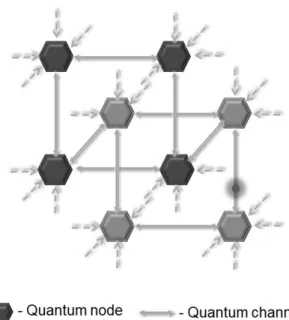
The ability to store, process and transfer quantum information which consists of quantum states and entanglement across long distances is one of the most lucrative applications that quantum sciences have to offer [60, 61]. The concept of quantum networks to facilitate this was introduced around two decades ago and since then a lot of progress has been made both theoretically and experimentally [62]. A quan-tum network comprises of individual quanquan-tum nodes that can generate, process and store quantum information which can then be communicated via quantum channels across multiple nodes as depicted by the schematic in Fig. 1.1. These quantum nodes play the role of quantum interfaces which interact with information carrying quantum channels. Most quantum communication protocols involve photonic qubits as information carries in optical channels. Though photons are ideal for

(28)

transport-Figure 1.1: Schematic of a Quantum Network: This is a cartoon representation of a quantum network where different quantum information carrying channels are in-terconnected with quantum interfaces made of physical systems that are capable of storing, processing and releasing quantum information carried in the quantum chan-nels.

ing information, it is extremely difficult to store and manipulate them. Therefore, the need of quantum nodes made of physical systems that can interact with photons and convert them into stationary material qubits that can be stored and efficiently converted back to carrier photons. Many systems are being investigated as potential quantum interfaces such as room temperature or cold atomic ensembles [63], trapped ion systems [64], solid state ensembles [65], quantum dots [66] and NV centers [67]. Of all these systems, atomic ensembles have been most well studied for applications as quantum interfaces. Atomic ensembles are easier to trap and manipulate using sim-ple linear optics and interact efficiently with information carrying photons. Quantum atomic ensembles provide a way to coherently convert a photonic qubit to an atomic qubit and vice-versa using schemes involving Raman transitions and Electromagneti-cally Induced Transparency (EIT) [41]. For a good review of different protocols used for storing and retrieving photons coherently from atomic ensembles refer the article by Hammerer et. al. [63]. Apart from efficient quantum interfaces, another

(29)

impor-tant requirement for quantum communication is the ability to improve state transfer across multiple quantum nodes. Quantum repeater protocols have been formulated to achieve this long distance states transfer using atomic ensembles and light-matter interactions [36]. More discussion on quantum repeaters and a brief explanation of the Duan-Lukin-Cirac-Zoller protocol is provided in Chapter III.

1.3 Outline of the Dissertation

Having laid out the basic concepts that will be important for the discussions in the following Chapters, let us now look at the organization of this dissertation. In Chapter II, we will be looking at a protocol to create multi-atom entangled Greenberger-Horne-Zeilinger (GHZ) states using Stimulated Raman Adiabatic Passage (STIRAP) and Rydberg blockade. The concepts of STIRAP and Rydberg blockade will be discussed before delving into the details of the protocol. In Chapter III we will study intrinsic retrieval efficiency of quantum interfaces formed from atomic ensembles that play an important role in quantum repeater protocols. A brief introduction to Duan-Lukin-Cirac-Zoller (DLCZ) quantum repeater protocol will also be provided in this Chapter. In Chapter IV, we will conclude with a discussion of the impacts of studying these two avenues exploring light-matter interactions in neutral cold-atom ensembles. Future outlook and improvements that can be made in these approaches will also be discussed.

(30)

CHAPTER II

Generating GHZ States in Atomic Ensembles

using STIRAP and Rydberg Blockade

2.1 Introduction

In this chapter, we will propose a protocol for the creation of multi-particle Greenberger-Horne-Zeilinger (GHZ) states in an atomic ensemble of three level Λ atoms using Stimulated Raman Adiabatic Passage (STIRAP) and Rydberg blockade. The effects of spontaneous emissions from excited atomic levels are also studied along with numerical results on the performance of this protocol.

We start this chapter by providing a brief introduction to GHZ states, the process of STIRAP and Rydberg blockade. It is then followed by the description of the main protocol and we conclude with discussion of the numerical results obtained for this method.

2.1.1 Greenberger-Horne-Zeilinger (GHZ) States

At the heart of quantum mechanics lies the phenomenon of quantum entangle-ment. Bell states, which are maximally entangled two qubit states show ‘measurement correlations stronger than could ever exist between classical systems’ in the words of Neilson and Chuang [61]. These non-classical correlations are the essence of Bell’s

(31)

inequalities that were formulated by John Bell in 1964 [68] addressing the paradox raised by Einstein-Podolsky-Rosen (EPR) in their famous paper on nature of phys-ical reality described by quantum mechanics[69]. Bell states play a central role in many quantum communication protocols like quantum teleportation, quantum key distribution etc. [20, 21, 61, 70–73]. Let us look at one of the four Bell states given below in Eq. (2.1).

|Φi= |00i√+|11i

2 (2.1)

Bell states show perfect correlation between the measurement results of the first qubit and the second qubit in any given basis irrespective of the physical separation between the two qubits. For example, in Eq. (2.1) whatever be the outcome of the measurement on the first qubit in a given basis, the outcome of the measurement of the second qubit is instantaneously determined. This perfect correlation in measurements violates the notion of local realism [68] and is the peculiar phenomenon at the heart of the EPR paradox.

Generalizations of these two qubit Bell states are the multi-particle entangled quantum states called the Greenberger-Horne-Zeilinger (GHZ) states given in Eq. (2.2) [74, 75].

|GHZim =

|0i⊗m_{± |1i}⊗m

√

2 , m >2 (2.2)

They exhibit entanglement based effects which are much more rich compared to Bell states [74–77]. Consider for example a three qubit GHZ state given in Eq. (2.3).

|GHZi3 =

|000i+|111i √

2 (2.3)

(32)

times we get the unentangled pure state |00i and the pure state|11irest of the time. On the other hand, taking a trace over one of the qubits leads to an unentangled mixed state whose density matrix is given in Eq. (2.4)

Tr1(|GHZi33hGHZ|) =

|00ih00|+|11ih11|

2 (2.4)

If instead of measuring one of the qubits of the three qubit GHZ state in the standard basis, one measures it in superposition basis |±i where:

|+i= |0i√+|1i

2 (2.5)

|−i= |0i − |1i√

2 (2.6)

we would get maximally entangled two qubit Bell states |00i ± |11i√

2 with a probability of one half each.

These highly entangled GHZ states violate Bell-like inequalities more strongly than their two qubit counter parts [76, 77]. The multi-particle entangled GHZ state shows unique non-local correlations which are essential for understanding the funda-mental principles of quantum entanglement [74, 78]. Exploration of unique non-local properties shown by GHZ states is a topic of ongoing research and will hopefully help define multi-particle quantum entanglement more concretely [79–81].

Like Bell states, GHZ states are important for various applications of quantum communication, cryptography and precision measurements [82–88]. With this short introduction to GHZ states, their important properties and applications, let us now briefly look at the concept of STIRAP.

(33)

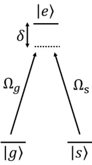
2.1.2 Stimulated Raman Adiabatic Passage (STIRAP)

The method of STIRAP introduced in the 1980s is a well known technique that allows a robust method of population transfer between two specific levels of a (gener-ally, three level) atomic system [89–91]. Consider a three level Λ atomic system shown in Fig. 2.1 such that the two levels|giand |siare stable or meta-stable states and|ei is an excited state. The transitions between states |gi − |ei are driven by a classical probe field and the transitions between the |si − |ei states by a similar pump field. The strength of both the pump and probe fields change as a function of time. Let

δg/sbe the detuning between the transition frequency and the carrier frequency of the

applied optical fields for the|gi − |ei and|si − |ei transitions respectively. Under the two photon resonance condition which implies that δ ≡ δg−δs = 0 as illustrated in

Fig. 2.1, the Hamiltonian of the system in the Rotating Wave Approximation (RWA) for a basis set {|gi,|ei,|si} is given in Eq. (2.7)

H = ~ 2       0 Ωg(t) 0 Ωg(t) 2δ Ωs(t) 0 Ωs(t) 0       . (2.7)

Where Ωg(t) is the time dependent Rabi frequency corresponding to the |gi − |ei

transition and similarly Ωs(t) is the Rabi frequency for the |si − |ei transition. We

have chosen the Rabi frequencies to be real for the sake of simplicity. One of the eigenergies of the above Hamiltonian in Eq. (2.7) is 0. The corresponding eigenstate of the Hamiltonian which has been traditionally called the Dark state, |Di given in Eq. (2.8) is at the center of this population transfer protocol.

|D(t)i= _q Ωs(t) Ω2 g(t) + Ω2s(t) |gi − _q Ωg(t) Ω2 g(t) + Ω2s(t) |si (2.8)

(34)

Figure 2.1: Λ atomic level structure: The states |gi and |si are two stable ground states that interact with the excited state |ei through Rabi frequencies Ωg and Ωs

respectively. Under the two photon resonance condition, the detuning for transitions |gi − |ei and |si − |ei is equal given by δ

We can simplify the analysis by considering the substitution tanθ(t) = Ωg(t) Ωs(t)

. The dark state can now be re-written as given below:

|D(t)i= cosθ(t)|gi −sinθ(t)|si (2.9)

Notice that state |Di has no contributions from the excited state|ei. If we start out with the atomic population in the state|gi, we can transfer it to state|siby adiabati-cally changing the co-efficients of the dark state from cosθ(0) = 1 to sinθ(T) = 1 over a duration of time period T in Eq. (2.9), with negligible occupation of the excited state. To enable this, optical fields controlling the |si − |ei transitions are turned on first, followed by the field for |gi − |ei transition. It is important that these fields are turned on and off adiabatically with sufficient temporal overlap between them to facilitate complete population transfer[89]. Since, the fields corresponding to Rabi frequency Ωs(t) is turned on first even though the atomic population is occupying the

(35)

[90, 92]. Unlike schemes of atomic population transfer where in precise control of the pulse shapes and intensities are required for high fidelity transfer, STIRAP is immune to minor fluctuations in these experimental conditions [89]. Thus, STIRAP is a robust method of population transfer from one state to another with extremely small loses due to spontaneous emission from the excited levels. Population trans-fer efficiency of more than 95% has been reported in numerous experiments using STIRAP [93–95]. Since, it is an adiabatic process, a discussion about the conditions required to maintain adiabaticity is important and they will be discussed in detail in the forthcoming Sec. 2.2.3. For a comprehensive review on STIRAP please refer to Vitanov et. al. [89]. Let us now briefly discuss the second important piece of our proposed GHZ state generation protocol, namely Rydberg blockade.

2.1.3 Rydberg Blockade

Rydberg atoms allow atomic excitation of the electrons to atomic levels with large principal quantum numbers, n1. Since the size of the atom scales as n2_,

atoms excited to high lying states have a large size and therefore a large dipole moment. These large dipole moments provide a controllable means of generating strong dipole-dipole interactions between Rydberg atoms [41, 42, 96]. The strong resonant dipole-dipole interactions scale as 1

R3 at short distances, R, and scale as

1

R6 corresponding to Van der Waals interactions at long distances [96]. This novel

feature of Rydberg atoms where the interactions can be turned on and off based on whether the atoms are excited to Rydberg levels or not plays an important role in many quantum information protocols to entangle atoms [41, 43, 97, 98].

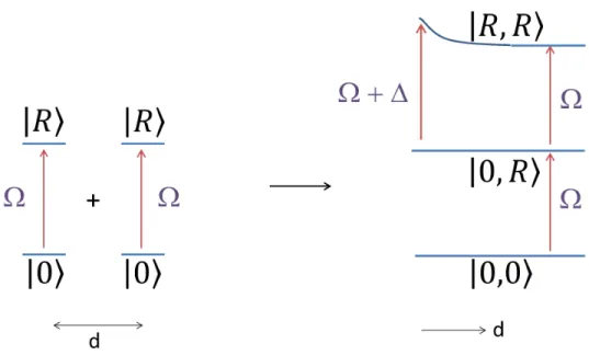
In an ensemble of neutral atoms, when two atoms are excited to Rydberg energy levels, because of the strong resonant dipolar interactions between them, the energy of doubly occupied Rydberg levels shifts. This energy shift is a function of the atomic dipole moment as well as the separation between the atoms. As a result, Rydberg

(36)

atoms in the vicinity of an excited Rydberg atom cannot be excited to the same Rydberg state because of these energy level shifts [96, 99]. It is explained pictorially in Fig. 2.2; because of the dipolar interaction between the two Rydberg atoms with a Rabi frequency Ω, the energy level with both the atoms excited to Rydberg level |R, Riundergoes an energy shift given by ∆ as a function of their inter-atomic distance

d. Notice that there is no effect on the energy levels when only one atom is excited to the Rydberg level and the other is in the ground state |0, Ri. This phenomenon of ‘dipole blockade’ provides an atomic control that acts on multiple atoms at the same time, which is necessary for generating entanglement between the atoms of the ensemble within the blockade radius. A blockade radius can be thought of as the radius of the sphere around an excited Rydberg atom within which no other atom can be excited to the Rydberg level with optical transitions. Thus, in essence only one Rydberg excitation is allowed within this sphere giving rise to a super-atom with multiple atoms. We will be using this phenomenon of Rydberg blockade as a controllable means of generating one step entanglement on a mesoscopic scale.

Let us now get into the details of the scheme for GHZ state generation using STIRAP and Rydberg blockade.

2.2 Proposal for GHZ state generation

Many ingenious schemes for creation of GHZ states in atomic systems have been previously proposed using a multi-step or a single-step process [96, 100, 101]. We present here a single-step scheme for GHZ state creation employing Rydberg dipole blockade and STIRAP [89, 102] using a single control atom and an ensemble of target atoms. Approaches to create a multi-particle GHZ state by using Electromagnetically Induced Transparency (EIT) and adiabatic passage along with Rydberg blockade have been previously studied [97, 98, 100]. Fidelity of the GHZ states obtained at the end of these protocols is an important parameter to consider. Because of radiative decay

(37)

Figure 2.2: Schematic of Rydberg blockade: When two Rydberg atoms with ground state |0i and excited Rydberg level |Ri are brought in close proximity, the energy level corresponding to the doubly excited|R, Ristate undergoes a distance dependent shift given by ∆. For values of inter-atomic separation, d, smaller than the blockade radius, excitation of two Rydberg atoms to the excited state is prohibited for a Rabi frequency Ω corresponding to the |0i − |Ritransition.

from the excited Rydberg states of the ensemble atoms, the fidelity of the GHZ states obtained in these schemes is adversely affected [96].

Here we propose a different theoretical scheme to realize the creation of a multi-particle GHZ state in an ensemble of Λ three-level Rydberg atoms which is robust to radiation decay from the excited Rydberg levels of the ensemble atoms. In this setup, the control atom and the ensemble of the target atoms are assumed to be independently addressable. This can be achieved by storing them in two separate trapping potentials in close proximity or in a lattice where the control atom can be efficiently addressed. This setup is similar to what has been discussed in the proposal by Muller et. al. [100].

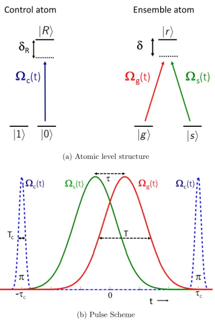
The control atom has a three level structure as is shown in Fig. 2.3a. The two meta-stable levels |0i and |1i determine the state of the control atom. Level |0i is connected to the excited Rydberg level |Ri via a control pulse with Rabi frequency

(38)

given by Ωc(t).

Level |1i is chosen such that dipolar transitions between |1i and |0i as well as |Ri are forbidden. An ensemble having N target Rydberg atoms is considered to be within the blockade radius of the excited control atom. The level structure of the ensemble atoms and the corresponding pulse sequence acting on them is shown in Fig. 2.3. Every ensemble atom has two metastable ground states, namely, |gi and |si and one Rydberg excited level|ri. All the ensemble atoms are initiated in the|gi state. This GHZ state creation protocol begins with a control π pulse having Rabi frequency Ωc(t) which is used to excite the control atom. If the control atom is in

state |1i, the control pulse has no effect. On the other hand, if it is in state |0i, with the action of the control π pulse, the atom is excited to the Rydberg level |Ri. Due to the long range dipole-dipole interactions between the excited Rydberg level |Ri and Rydberg levels |ri, the target ensemble Rydberg levels undergo energy level shift given by a frequency ∆ (refer to Sec. 2.1.3). In the absence of this energy shift, the condition for adiabatic population transfer of the ensemble atoms from the ground state |gN_i ₌ _⊗N

j=1|gij to |sNi = ⊗Nj=1|sij via the counter-intuitive STIRAP pulse

sequence Ωs(t) and Ωg(t) [Fig. 2.3] is satisfied (refer to Sec. 2.1.2). The parameters

of the system are set up in such a way that when the control atom is excited to |Ri, the induced energy shift ∆ in the ensemble atoms disrupts the STIRAP condition for population transfer from |gN_i_to _|_sN_{i. Due to the added detuning the population}

remains in the state|gNiafter the application of the STIRAP pulses. Finally, another control π pulse is used to bring the control atom back to the original state. When the control atom is prepared in the _√1

2(|0i+|1i) superposition state at the beginning

of the protocol and finally measured in the superposition basis, the ensemble atoms get projected to a N particle GHZ state.

If the conditions for STIRAP are met, the instantaneous eigenstate occupied by the ensemble atoms has no contribution from the level |ri at all times. Hence, this

(39)

(a) Atomic level structure

(b) Pulse Scheme

Figure 2.3: Atomic level structure and pulse scheme for GHZ state generation: (a) This figure describes the atomic level structure of the control atom and the target ensemble atoms. The control atom has two metastable states |0i and |1i. The level |0i interacts with the excited Rydberg level |Ri via Rabi frequency Ωc(t). δR is

the detuning between the carrier frequency of the light pulse and the frequency of transition between the levels |0i and |Ri. The level |1i is isolated from the other levels. Each target atom has a Λ type level structure with two metastable states, |gi and |si. They interact with the excited Rydberg level |ri via Gaussian pulses having Rabi frequencies Ωg(t) and Ωs(t) respectively. The detuning for both the

pulses is given by δ. (b) This figure describes the pulse sequences for the GHZ state generation protocol. The protocol begins with a Gaussian [Ωc(t)] π pulse having a

standard deviation given by Tc to take the control atom from |0i to |Ri. It is then

followed by counter-intuitive STIRAP pulse sequence with Gaussian profiles, each havingT(Tc) standard deviation. τ is the time interval between the peaks of these

(40)

protocol is insensitive to the radiative decay losses from the excited Rydberg level of the ensemble atoms.

Let us now analyze this scheme in detail and study the dependence of the STIRAP transfer conditions on the parameters of the system. In Sec. 2.2.1 we discuss the dynamics of the control atom. This is followed by the discussion of the transfer mechanism in the target atoms and the adiabaticity conditions required for efficient transfer in Sec. 2.2.2. Numerical simulations of this protocol for realistic parameters are then presented in Sec. 2.3 . In Sec. 2.5 we conclude the discussion.

2.2.1 The control atom

Hamiltonian for the control atom interacting with the classical control field in the field interaction representation with the Rotating Wave Approximation (RWA) is given below: HC(t) ~ = δR|RihR|+ Ω∗_c(t) 2 |0ihR|+ Ωc(t) 2 |Rih0| (2.10)

The energy levels are measured relative to the ground state energy _~ω0 = 0. In Eq.

(2.10), δR ≡ ωR −ωc is the detuning between the frequency of transition from |0i

to |Ri (denoted by ωR) and the optical frequency of the control pulse, ωc. As noted

previously, Ωc(t) is the Rabi frequency of the control pulse with a Gaussian temporal

profile given below.

Ωc(t) = Ωc0exp −(t−τc) 2 2T2 c (2.11)

We will assume the peak Rabi frequency, Ωc0, to be real in all the calculations here

after. As already noted, level |1i is isolated from the levels |0i and |Ri and hence is not included in the Hamiltonian. For δR = 0, on solving the Schrodinger’s equation

(41)

For complete transfer of population from|0ito|Ristate, Θ should be an odd multiple of π 2. Thus, we need: Ωc0Tc = (2p+ 1) r π 2, p∈Z (2.15)

To check for the robustness of this transfer against variations in the Rabi frequency, we look at the derivative of |cR(∞)|with respect to Ωc0.

∂|cR(∞)| ∂Ωc0 = −Tc r π 2 cos(Ωc0Tc r π 2) (2.16)

Eq. (2.16) implies that smaller values ofTcprovide more robustness against variation

in Ωc0. For δR 6= 0, analytic solution for Gaussian form of the Rabi frequency is

difficult to derive. Hence, we will look at the dependence of |cR(∞)|2 on different

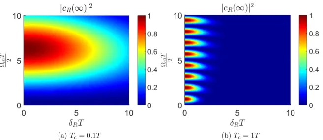
values of Ωc0, δR and Tc numerically in Fig. 2.4. For the value of Tc = 0.1T, where

T is the standard deviation of the Gaussian STIRAP pulses, we see from Fig. 2.4a that the population gets completely transferred to the |Ri state when Ωc0T

2 = 6.2 and δRT = 0. From Fig. 2.4b, we see that there are multiple periodic values of Ωc0T

for which complete population transfer to the excited level can be achieved via a π

pulse as expected from Eq. (2.15) for Tc = 1T. As δRT becomes larger, the fraction

of population in the excited state decreases and eventually becomes zero. The effect of larger values of δRT is more prominent for larger values of Tc. As derived in Eq.

(42)

(a)Tc = 0.1T (b)Tc= 1T

Figure 2.4: Population distribution of the control atoms for different values of detun-ing and Rabi frequencies: (a) The coefficient of population in state |Ri transferred from |0i, |cR(∞)|2, due to the control π pulse is plotted as a function of scaled

de-tuning δRT and scaled peak control Rabi frequency Ωc0T for a value of Tc = 0.1T.

(b) Same as plot (a) but for value of Tc = 1T. We see that smaller values of Tc are

more robust to variations in detuning and peak Rabi frequency.

(2.16), we see that smaller values ofTcprovide more robust transfer against variations

in Ωc0 and δR.

2.2.2 The target ensemble

In this section, we will derive the conditions that are necessary to maintain adia-batic transfer of the ensemble atoms from |gN_i _to _|_sN_i _{when the control atom is in}

state |1i and to remain in the state |gNi when the control atom is in the |0i state. The Hamiltonian for ensemble atoms interacting with the counter-intuitive STIRAP pulse sequence in the RWA is given below:

(43)

In Eq. (2.17), _~ω0

r is the energy of the excited level |ri. For the energy of states |gi

and|sidenoted by_~ω0

g and~ω0s respectively,δg(s)=ωr0−ωg0(s)−ωg(s)are the detunings

of these levels with respect to the optical frequenciesωg andωs of the STIRAP pulses

shown in Fig. 2.3b. The corresponding Rabi frequencies Ωg(t) and Ωs(t) are defined

as follows: Ωg(t) = Ω exp − (t− τ 2) 2 2T2 (2.18) Ωs(t) = Ω exp − (t+ τ 2) 2 2T2 (2.19)

In Eqs. (2.18)-(2.19), Ω is the peak Rabi frequency of the Gaussian STIRAP pulses,

τ is the time separation between the peaks of the two pulses and T is the standard deviation. We can simplify the Hamiltonian in Eq. (2.17) by setting ω0

r = 0 and

assuming two photon resonance condition for the system i.e. δg = δs = δ [102].

Boosting the energy of all the levels by δ, we get the modified Hamiltonian for the target ensemble as:

HT(t) ~ = N X j=1 δ|rijhr|+ Ω∗_g(t) 2 |gijhr|+ Ω∗_s(t) 2 |sijhr|+ h.c. (2.20)

We will restrict the set of basis states for the analysis of this system to a set containing only one Rydberg level excitation by assuming that all the atoms are within the Rydberg blockade radius of each other. We can rewrite the Hamiltonian in Eq. (2.20) in the symmetric Fock state basis set defined by [103]:

(44)

In the above equation, a†_µis an operator for creation of atomic excitation in the state

µand similarly, aν is the destruction operator. There are in all (2N+1) states in this

basis set, namely,

|g;s;riN =

|gN;s0;r0i, ..,|gN−n;sn;r0i, ..|g0;sN;r0i,

|gN−1;s0;r1i, ..,|gN−n−1;sn;r1i, ..|g0;sN−1;r1i (2.24)

As a short hand notation, we use |gNi ≡ |gN;s0;r0i and |sNi ≡ |g0;sN;r0i. The corresponding Hamiltonian in the Fock number basis is then:

HT(t) ~ = δσ + r σ − r + Ω ∗ g(t) 2 a † gσ − r + Ω∗_s(t) 2 a † sσ − r + h.c. (2.25) Where: σ_r+|r0i = |r1i, σ_r−|r0i = 0 (2.26) σ_r−|r1i = |r0i, σ_r+|r1i = 0 (2.27)

Using the properties of block [104] and tri-diagonal matrices [105] it can be shown that the Hamiltonian in Eq. (2.25) when expressed as a matrix in the basis set defined by Eq. (2.24) always has one eigenvalue as 0. The characteristic equation for this Hamiltonian is invariant when δ → −δ and the eigenvalue λ → −λ. The details of finding the eigenvalues of the Hamiltonian given in Eq. (2.25) in the basis set defined in Eq. (2.24) is provided in Appendix A. With the following new definitions given in Eqs. (2.28)-(2.29), let us explore the eigen-structure of this system.

Ω0(t) ≡ q Ω2 g(t) + Ω2s(t) (2.28) tanθ(t)≡ Ωg(t) Ωs(t) ; tanϕ(t)≡ Ω0(t) δ (2.29)

(45)

On solving for the eigenvalues of this system, we find that the non-zero eigen-energies are (refer to Appendix A for details):

E_±N_n = ~Ω0(t)

2 [cotϕ(t)±

q

n+ cot2_ϕ₍_t_)]_{, n}_{= 1}_{, .., N} _(2.30)

The corresponding eigen-states are denoted by|λN

±ni. The eigenstate with eigenenergy

0 is given as: |O(t)i = N X n=0 (−1)N−n_αN n(t)|g N−n_;_sn_;_r0_i _(2.31) αN_n(t) = s N! n!(N −n)!cos N−n₍_θ₍_t_{)) sin}n₍_θ₍_t₎₎ _(2.32)

State |O(t)i is the N particle STIRAP state. As t → −∞, |O(−∞)i = |gN_i _and

t → ∞, |O(∞)i= |sN_{i. If this system evolves adiabatically, then the population of}

the target ensemble can be coherently transferred from |gNi to|sNi. This eigenstate with eigenvalue 0 has no contribution from the excited level |ri for any number of ensemble atoms at all times. It is also independent of the detuningδ. In the STIRAP process our aim is to keep the target ensemble in the instantaneous eigenstate|O(t)i at all times. Adiabatic population transfer along this eigenstate implies that this protocol is insensitive to the spontaneous emissions from the excited level|ri. This is a key feature of this scheme which provides us with a robust mechanism of population transfer even in the presence of decay. Numerical studies in the presence of decay are described in Sec. 2.3.

2.2.3 Adiabaticity conditions

Let us now look at the adiabaticity conditions required for the desired population transfer. The condition for maintaining adiabatic transfer along the |O(t)i state is

(46)

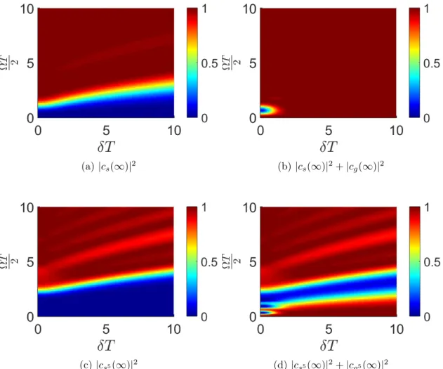
(a)|cs(∞)|2 (b)|cs(∞)|2+|cg(∞)|2

(c)|cs5(∞)|2 (d)|c_s5(∞)|2+|c_g5(∞)|2

Figure 2.5: Population distribution of ensemble atoms in the multi-particle ground states |gN_i _and _|_sN_{i: (a) Co-efficient of population in state} _|_s_i _{for a target ensemble}

with 1 atom after the application of STIRAP pulses as a function of the scaled peak Rabi frequency ΩT and scaled detuning δT for τ = 1.4T.(b)Total population in the state |si and |gi after the STIRAP pulses for a single target atom as a function of ΩT and δT. (c) Same as plot (a) but for a target ensemble of 5 atoms. (d) Same as plot (b) for N = 5 atoms. We see that as the number of target atoms goes up, the parameter space for adiabatic transfer from|gN_i_to_|_sN_i_{or no transfer gets modified}

(47)

summarized by the adiabaticity criterion discussed in [106] given as: X m6=0 ~ hm|O˙(t)i E0 −Em 1 (2.33)

In the above Eq. (2.33), E0 is the eigenenergy of the eigenstate |O(t)i and the sum

is taken over all the other eigenstates|mi with eigenenergiesEm.

From here onwards, we will assume Ω to be real. On analyzing the eigenstates |λN±1i corresponding to eigenenergies E±N1, we find that the projection of state |λN±1i

onto the |r0_i _{subspace is co-linear with} _|_O_˙₍_t_)i:

hλN₊₁(t)|O˙(t)i = θ˙(t)√Nsin(ϕ(t)

2 ) (2.34)

hλN₋₁(t)|O˙(t)i = θ˙(t)√Ncos(ϕ(t)

2 ) (2.35)

The eigen-structure is such that for any value of N, all the eigenstates except the zeroth eigenstate have non-zero projections in the |r1_i _{subspace. From the}

orthonor-mality properties of the eigenvectors we can deduce that:

hλN_±_n|P_r0P† r0|λ N ±mi=hλ N ±n|Pr1P† r1|λ N ±mi= 0 ∀ n6=m (2.36) Here, P_r†0 and P †

r1 are projection operators for the|r0iand|r1isubspace respectively.

From the above deduction we can conclude that only the|λN_±₁ieigenstates contribute to the sum in Eq. (2.33). On simplifying the adiabatic condition we get:

˙ θ(t) Ω0(t) 2√Nf(ϕ(t)) (2.37) f(ϕ(t)) = sin ϕ(t) 2 cos ϕ(t) 2 sin3ϕ(₂t) + cos3 ϕ(t) 2 (2.38)

(48)

condi-tion is rewritten in Eq. (2.39). Here, we have scaled all the variables with T, thus, ˜

Ω≡ΩT, ˜τ ≡ τ

T and similarly ˜δ and ˜t.

1 r 2 N ˜ Ω ˜ τ exp (− (˜t2+ ˜τ₄2) 2 ) cosh 3/2 (˜tτ˜)f(ϕ(˜t)) (2.39)

Since, the Rabi frequencies and detuning are positive, 0≤ϕ(t)< π

2. The function

f(ϕ(t)) is a monotonically increasing function of ϕ(t) in this range. For the strictest adiabaticity condition, we should choose the limit when ϕ(t) → 0. In this limit,

f(ϕ(t)) = Ω0(t)

2δ , given δ Ω0(t). On the other hand, when ϕ(t) → π

2, we get

f(ϕ(t)) = √1

2 with δ → 0. For the duration of population transfer, i.e. when Ω0(˜t)

is considerably large, the ˜t dependence of the RHS of Eq. (2.39) varies from being singly peaked with maximum at ˜t = 0 till ˜τ is increased from 0 to about 1.4, to being doubly peaked as ˜τ is increased further with a minimum at ˜t = 0. It is thus sufficient to study the Eq. (2.39) at ˜t= 0 for all values of ˜τ. Incorporating the above simplifications, the adiabaticity condition now is given as:

1 Ω˜ 2 √ Nτ˜˜δexp (− ˜ τ2 4 ) when ˜δ ˜ Ω (2.40)

It is worthwhile to keep in mind that when δ →0, this condition becomes:

1 √Ω˜

N˜τ exp (−

˜

τ2

8 ) (2.41)

Note the dependence of the adiabaticity conditions in Eq. (2.40) and Eq. (2.41) on the number of atoms in the ensemble. The condition for adiabatic transfer along the |Oi eigenstate becomes stricter by √N for an ensemble of N atoms. The optimum value of τ can be obtained numerically. When all other parameters are fixed, the condition ˜δΩ˜2 for the adiabatic transfer is similar to what was proved by Vitanov and Stenholm in 1997 [91] for a single atom case.

(49)

Let us now understand the condition required for the atomic population to remain in the state |gN_i _{when the added detuning due to Rydberg dipole-dipole interaction}

is introduced. For a single atom case, as long as ˜δ Ω, we can reduce the three level˜ system to a two level system. In this case, the condition for adiabatic transfer from|gi to|siis simply ˜δ Ω˜2_{, ignoring the effects of ˜}_τ_{. On the other hand, the condition to}

remain in the |gi state is ˜Ω2 ˜δ which is obtained by making the effective coupling between levels |gi and |si small [91]. This situation changes a little in the presence of more than one atom. In this case, when we enforce that the effective couplings are kept small, the condition for the ensemble state to remain in the state |gN_i _is

modified to:

√

NΩ˜2 δ˜when ˜Ωδ˜ (2.42)

Thus, we can conclude that for the ensemble state to be transferred to |sN_i _state

from the initial state|gN_{i, assuming ˜}_τ _{is fixed, we must have:}

˜ δ|1i ˜ Ω2 √ N when ˜δ|1i ˜ Ω (2.43) 1 √Ω˜ N when ˜δ|1i →0 (2.44)

Also, for the ensemble state to remain in the |gN_i _{state, we must have:}

˜

δ|0i

√

NΩ˜2 when ˜δ|0i Ω˜ (2.45)

In the above equations ˜δ|0i and ˜δ|1i are the detunings of ensemble atoms when the

control atom is in state |0i and |1i respectively. For our protocol to work efficiently, our system should satisfy the conditions given in Eq. (2.43) or Eq. (2.44) along with Eq. (2.45). Thus, we can take ˜δ|0i= ˜δ|1i+ ˜∆.

(50)

sec-tion, we numerically evolve the Hamiltonian for the ensemble atoms given in Eq. (2.25) for different values of ΩT and δT. In Fig. 2.5 we plot the population of en-semble atoms in state |sN_i _for _N _{= 1 and 5 denoted by the co-efficient} _|_c

sN(∞)|2.

To compare this with the population that remained in the initial state |gN_{i, we plot}

the total population in the states|sN_i_and _|_gN_i _{after the completion of the protocol.}

This sum is denoted as |cgN(∞)|2+|c_sN(∞)|2. ForN = 1, we see from Fig. 2.5a, the

population gets completely transferred to |si state for ˜Ω2 δ˜. It is clear from Fig. 2.5b, there is only a small portion of the parameter space when Ω˜₂ ≈˜δ <3 where adi-abatic transfer of population as described above does not take place for N = 1. This situation changes as the number of atoms in the target ensemble increases since more intermediate states now become available. For N = 5, as seen from Fig. 2.5c, the condition for adiabatic transfer from |g5_i _to _|_s5_i _{becomes stricter compared to that}

for N = 1. Portions of the parameter space defined by ˜Ω and ˜δ open up where the adiabaticity conditions fail. This region clearly divides the parameter space into two sections, one which allows the adiabatic transfer of population from|gNito|sNiwith high fidelity marked out by the condition ˜Ω2 √_N_δ_˜_{and the other where population}

remains in|gN_i_{with unit probability. The Rydberg-Rydberg interaction between the}

control and the ensemble atoms provides a tunable mechanism to increase or decrease the effective value of ˜δ such that the target atoms are always in either of these two high fidelity transfer regions subject to the state of the control atom.

2.3 Introduction of spontaneous emissions

Before we start analyzing the numerical simulations for the control and target sys-tem together, let us introduce the effect of decoherence due to spontaneous emissions from the excited Rydberg states for the control atom and the target ensemble.

(51)

number of spontaneous emission decay channels is given below: ˙ ρ = i ~[ρ, H] + ˆL(ρ) (2.46) ˆ L(ρ) = −1 2 M X m=1 (C_m†Cmρ+ρCm†Cm)+ M X m=1 CmρCm† (2.47)

For the control atom, we have only one decay channel with the decay rate Γ0R, namely,

ˆ

C0R = p

Γ0R|0ihR| (2.48)

For the target ensemble atoms, there are two decay channels with rates Γgr and Γsr

defined as: ˆ Cgr = p Γgr|gihr| (2.49) ˆ Csr = p Γsr|sihr| (2.50)

In the forth coming numerical calculations, we have chosen Γgr = Γsr ≡ Γr. It is

straight-forward to extend the master equation calculations for a system with more than one target atom using the Fock number state basis.

We will first study the effect of decay due to spontaneous emissions on the target ensemble with different number of atoms. We choose the value of T = 1µs and ˜

τ = 1.4 for all the numerical results here after. From Fig. 2.6, we see that even for an ensemble of about ten atoms, the population transferred to the |sNi state from the |gNi state is greater than 99% for realistic values of Rydberg level spontaneous emission rates of about Γr ≈ 0.01−0.1 MHz. As discussed above, we see that the

spontaneous emissions from the Rydberg excited levels of the target ensemble atoms do not affect this protocol which makes it a very robust scheme.

(52)

Figure 2.6: Effect of spontaneous emissions on ensemble atoms: The population in level |sN_i _{after the STIRAP pulses for different number of atoms in the target}

ensemble, N, and varying spontaneous emission rate ΓrT. The value of detuning

δT = 0, Ω₂T = 9.5 and τ = 1.4T. We see that the population transfer does not depend on the decay rate significantly and has values higher than 0.99 for typical range of ΓrT ≈0.01−0.1

2.4 Numerical results for GHZ state creation

Having laid the groundwork we will now look at the simulation of GHZ state creation. The total Hamiltonian for this system is:

HT ot(t) = HC(t) +HT(t) +~∆|RihR|σr+σ

−

r (2.51)

The expressions for HC(t) and HT(t) are given in the Eq. (2.10) and Eq. (2.25)

respectively. The interaction between the target ensemble and the control atom is introduced via the last term in Eq. (2.51) with the interaction strength given by frequency ∆. Ideally, ∆ is a function of inter-atomic separation. In this case we can choose the value of ∆ such that it defines the threshold for the blockade radius. All atoms in the ensemble will have a detuning greater than this value. The exact value of ∆ is not important as long as it is large enough to avoid two Rydberg atom