Active Inference, Curiosity and Insight

(1)

Active Inference, Curiosity and Insight

Karl J. Friston

k.friston@ucl.ac.uk Marco Lin

marco.lin91@gmail.com

Wellcome Trust Centre for Neuroimaging, Institute of Neurology, University College London WC1N 3BG, U.K.

Christopher D. Frith c.frith@ucl.ac.uk

Wellcome Trust Centre for Neuroimaging, Institute of Neurology, University College London WC1N 3BG, and Institute of Philosophy, School of

Advanced Studies, University of London EC1E 7HU, U.K. Giovanni Pezzulo

giovanni.pezzulo@gmail.com

Institute of Cognitive Sciences and Technologies, National Research Council, 7-00185 Rome, Italy

J. Allan Hobson

allan_hobson@hms.harvard.edu

Wellcome Trust Centre for Neuroimaging, Institute of Neurology, University College London WC1N 3BG, U.K., and Division of Sleep Medicine,

Harvard Medical School, Boston, MA 02215, U.S.A. Sasha Ondobaka

s.ondobaka@ucl.ac.uk

Wellcome Trust Centre for Neuroimaging, Institute of Neurology, University College London WC1N 3BG, U.K.

This article offers a formal account of curiosity and insight in terms of active (Bayesian) inference. It deals with the dual problem of inferring states of the world and learning its statistical structure. In contrast to cur-rent trends in machine learning (e.g., deep learning), we focus on how people attain insight and understanding using just a handful of observa-tions, which are solicited through curious behavior. We use simulations of abstract rule learning and approximate Bayesian inference to show that minimizing (expected) variational free energy leads to active sam-pling of novel contingencies. This epistemic behavior closes explanatory gaps in generative models of the world, thereby reducing uncertainty and

(2)

satisfying curiosity. We then move from epistemic learning to model se-lection or structure learning to show how abductive processes emerge when agents test plausible hypotheses about symmetries (i.e., invari-ances or rules) in their generative models. The ensuing Bayesian model reduction evinces mechanisms associated with sleep and has all the hall-marks of “aha” moments. This formulation moves toward a computa-tional account of consciousness in the pre-Cartesian sense of sharable knowledge (i.e.,con: “together”;scire: “to know”).

1 Introduction

This article presents a formal (computational) description of epistemic be-havior that calls on two themes in theoretical neurobiology. The first is the use of Bayesian principles for understanding the nature of intelligent and purposeful behavior (Koechlin, Ody, & Kouneiher, 2003; Oaksford & Chater, 2003; Coltheart, Menzies, & Sutton, 2010; Nelson, McKenzie, Cot-trell, & Sejnowski, 2010; Collins & Koechlin, 2012; Solway & Botvinick, 2012; Donoso, Collins, & Koechlin, 2014; Seth, 2014; Koechlin, 2015; Lu, Rojas, Beckers, & Yuille, 2016). The second is the role of self-modeling, reflection, and sleep (Metzinger, 2003; Hobson, 2009). In particular, we formulate cu-riosity and insight in terms of inference—namely, the updating of beliefs about how our sensations are caused. Our focus is on the transitions from states of ignorance to states of insight—namely, states with (i.e.,con) aware-ness (i.e.,scire) of causal contingencies. We associate these epistemic tran-sitions with the process of Bayesian model selection and the emergence of insight. In short, we try to show that resolving uncertainty about the world, through active inference, necessarily entails curious behavior and conse-quent ‘aha’ or eureka moments.

The basic theme of this article is that one can cast learning, inference, and decision making as processes that resolve uncertainty about the world. This theme is central to many issues in psychology, cognitive neuroscience, neuroeconomics, and theoretical neurobiology, which we consider in terms of curiosity and insight. The purpose of this article is not to review the large literature in these fields or provide a synthesis of established ideas (e.g., Schmidhuber, 1991; Oaksford & Chater, 2001; Koechlin et al., 2003; Botvinick & An, 2008; Nelson et al., 2010; Navarro & Perfors, 2011; Tenen-baum, Kemp, Griffiths, & Goodman, 2011; Botvinick & Toussaint, 2012; Collins & Koechlin, 2012; Solway & Botvinick, 2012; Donoso et al., 2014). Our purpose is to show that the issues this diverse literature addresses can be accommodated by a single imperative (minimization of expected free energy, or resolution of uncertainty) that already explains many other phenomena–for example, decision making under uncertainty, stochas-tic optimal control, evidence accumulation, addiction, dopaminergic re-sponses, habit learning, reversal learning, devaluation, saccadic searches,

(3)

scene construction, place cell activity, omission-related responses, mis-match negativity, P300 responses, phase-precession, and theta-gamma cou-pling (Friston, FitzGerald et al., 2016; Friston, FitzGerald, Rigoli, Schwarten-beck, & Pezzulo, 2017). In what follows, we ask how the resolution of un-certainty might explain curiosity and insight.

1.1 Curiosity. Curiosity is an important concept in many fields, includ-ing psychology (Berlyne, 1950, 1954; Loewenstein, 1994), computational neuroscience, and robotics (Schmidhuber, 1991; Oaksford & Chater, 2001). Much of neural development can be understood as learning contingen-cies about the world and how we can act on the world (Saegusa, Metta, Sandini, Sakka, 2009; Nelson et al., 2010; Nelson, Divjak, Gudmundsdottir, Martignon, & Meder, 2014). This learning rests on intrinsically motivated curious behavior that enables us to predict the consequences of our ac-tions: as nicely summarized by Still and Precup (2012), “A learner should choose a policy that also maximizes the learner’s predictive power. This makes the world both interesting and exploitable.” This epistemic, world-disclosing perspective speaks to the notion of optimal data selection and important questions about how rational or optimal we are in querying our world (Oaksford, Chater, Larkin, 2000; Oaksford & Chater, 2003). Clearly, the epistemic imperatives behind curiosity are especially prescient in de-velopmental psychology and beyond: ”In the absence of external reward, babies and scientists and others explore their world. Using some sort of adaptive predictive world model, they improve their ability to answer ques-tions such as what happens if I do this or that?” (Schmidhuber, 2006). In neu-rorobotics, these imperatives are often addressed in terms of active learning (Markant & Gureckis, 2014; Markant, Settles, & Gureckis, 2016), with a fo-cus on intrinsic motivation (Baranes & Oudeyer, 2009). Active learning and intrinsic motivation are also key concepts in educational psychology, where they play an important role in enabling insight and understanding (Eccles & Wigfield, 2002).

1.2 Insight and Eureka Moments. The Eureka effect (Auble, Franks, & Soraci, 1979) was introduced to psychology by comparing the recall for sentences that were initially confusing but subsequently understood. The implicit resolution of confusion appears to be the main determinant of re-call and the emotional concomitants of insight (Shen, Yuan, Liu, & Luo, 2016). Several psychological theories for solving insight problems have been proposed—for example, progress monitoring and representational change theory (Knoblich, Ohlsson, & Raney, 2001; MacGregor, Ormerod, & Chronicle, 2001). Both enjoy empirical support, largely from eye move-ment studies (Jones, 2003). Furthermore, several psychophysical and neu-roimaging studies have attempted to clarify the functional anatomy of insight (see Bowden, Jung-Beeman, Fleck, & Kounios, 2005), for a psycho-logical review and Dresler et al., 2015, for a review of the neural correlates of

(4)

insight in dreaming and psychosis). In what follows, we offer a normative framework that complements psychological theories by describing how cu-riosity engenders insight. Our treatment is framed by two questions posed by Berlyne (1954) in his seminal treatment of curiosity: ”The first question is why human beings devote so much time and effort to the acquisition of knowledge. . . . The second question is why, out of the infinite range of knowable items in the universe, certain pieces of knowledge are more ar-dently sought and more readily retained than others?” (p. 180).

In brief, we will try to show that the acquisition of knowledge and its retention are emergent properties of active inference—specifically, that cu-riosity manifests as an active sampling of the world to minimize uncertainty about hypotheses—or explanations—for states of the world, while reten-tion of knowledge entails the Bayesian model selecreten-tion of the most plausi-ble explanation. The first process rests on curious, evidence-accumulating, uncertainty-resolving behavior, while the second operates on knowledge structures (i.e., generative models) after evidence has been accumulated.

Our approach rests on the free energy principle, which asserts that any sentient creature must minimize the entropy of its sensory exchanges with the world. Mathematically, entropy is uncertainty or expected surprise, where surprise can be expressed as a free energy function of sensations and (Bayesian) beliefs about their causes. This suggests that creatures are com-pelled to minimize uncertainty or expected free energy. In what follows, we will see that resolving different sorts of uncertainty furnishes principled ex-planations for different sorts of behavior. These levels of uncertainty pertain to plausible states of the world, plausible policies that change those states, and plausible models of those changes.

The first level of uncertainty is about the causes of sensory outcomes under a particular policy (i.e., sequence of actions). Reducing this sort of uncertainty corresponds to perceptual inference (a.k.a. state estimation). In other words, the first thing we need to do is infer the current state of the world and the context in which we are operating. We then have to con-tend with uncertainty about policies per se that can be cast in terms of uncertainty about future states of the world, outcomes, and the probabilis-tic contingencies that bind them. We will see that minimizing these three forms of expected surprise—by choosing an uncertainty resolving policy— corresponds to information-seeking epistemic behavior, goal-seeking prag-matic behavior, and novelty-seeking curious behavior, respectively. In short, by pursuing the best policy, we accumulate experience and reduce uncertainty about probabilistic contingencies through epistemic learning— namely, inferring (the parameters of our models of) how outcomes are generated.

Finally, curious, novelty-seeking policies enable us to reduce our uncer-tainty about our generative models per se, leading to structure learning, insight, and understanding. Here, a generative model constitutes a hypoth-esis about how observable outcomes are generated, where we entertain

(5)

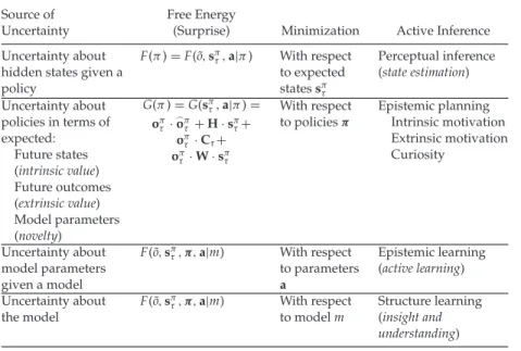
Table 1: Sources of Uncertainty Scored by (Expected) Free Energy and the Behaviors Entailed by Its Minimization (Resolution of Uncertainty through Approximate Bayesian Inference).

Source of Free Energy

Uncertainty (Surprise) Minimization Active Inference Uncertainty about

hidden states given a policy F(π)=F( ˜o,sπ_τ,a|π) With respect to expected statessπ_τ Perceptual inference (state estimation) G(π)=G(sπ_τ,a|π)= oπ_τ ·oπ_τ+H·sπ_τ+ oπ_τ ·Cτ+ oπ_τ ·W·sπ_τ Uncertainty about policies in terms of expected: Future states (intrinsic value) Future outcomes (extrinsic value) Model parameters (novelty) With respect

to policiesπ Epistemic planningIntrinsic motivation Extrinsic motivation Curiosity Uncertainty about model parameters given a model F( ˜o,sπ_τ,π,a|m) With respect to parameters a Epistemic learning (active learning) Uncertainty about the model F( ˜o,sπ_τ,π,a|m) With respect to modelm Structure learning (insight and understanding)

competing hypotheses that are, a priori, equally plausible. In short, the last level of uncertainty reduction entails the selection of models that render outcomes the least surprising, having suppressed all other forms of un-certainty. All but the last process require experience to resolve uncertainty about either the states (inference) or parameters (learning) of a particular model. However, optimization of the model per se can proceed in a fact-free, or outcome-fact-free, fashion, using experience accumulated to date. In other words, no further facts or outcomes are necessary for this last level of optimization: facts and outcomes are constitutive of the experience on which this optimization relies. It is this Bayesian model selection we asso-ciate with fact-free learning (Aragones, Gilboa, Postlewaite, & Schmeidler, 2005) and the emergence of insight (Bowden et al., 2005).

Table 1 provides a summary of these uncertainty-reducing processes, where uncertainty is associated with free energy formulations of surprise such that uncertainty-resolving behavior reduces expected free energy. To motivate and illustrate this formalism, we set ourselves the task of sim-ulating a curious agent that spontaneously learned rules—governing the sensory consequences of her action—from limited and ambiguous sensory evidence (Lu et al., 2016; Tervo, Tenenbaum, & Gershman, 2016). We chose abstract rule learning to illustrate how conceptual knowledge could be

(6)

accumulated through experience (Botvinick & Toussaint, 2012; Zhang & Maloney, 2012; Koechlin, 2015) and how implicit Bayesian belief updat-ing can be accelerated by applyupdat-ing Bayesian principles not to sensory samples but to beliefs based on those samples. This structure learning (Tenenbaum et al., 2011; Tervo et al., 2016) is based on recent developments in Bayesian model selection, namely, Bayesian model reduction (Friston, Litvak et al., 2016). Bayesian model reduction refers to the evaluation of re-duced forms of a full model to find simpler (rere-duced) models using only posterior beliefs (Friston & Penny, 2011). Reduced models furnish parsi-monious explanations for sensory contingencies that are inherently more generalizable (Navarro & Perfors, 2011; Lu et al., 2016) and, as we will see, provide for simpler and more efficient inference. In brief, we use simula-tions of abstract rule learning to show that context-sensitive contingencies, which are manifest in a high-dimensional space of latent or hidden states, can be learned using straightforward variational principles (i.e., minimiza-tion of free energy). This speaks to the nominimiza-tion that people ”use their knowl-edge of real-world environmental statistics to guide their search behavior” (Nelson et al., 2014). We then show that Bayesian model reduction adds an extra level of inference, which rests on testing plausible hypotheses about the structure of internal or generative models. We will see that this process is remarkably similar to physiological processes in sleep, where redundant (synaptic) model parameters are eliminated to minimize model complexity (Hobson & Friston, 2012). We then show that qualitative changes in model structure emerge when Bayesian model reduction operates online during the assimilation of experience. The ensuing optimization of model evidence provides a plausible (Bayesian) account of abductive reasoning that looks very much like an “aha” moment. To simulate something akin to an aha moment requires a formalism that deals explicitly with probabilistic beliefs about states of the world and its causal structure. This contrasts with the sort of structure or manifold learning that predominates in machine learn-ing (e.g., deep learnlearn-ing; LeCun, Bengio, & Hinton, 2015), where the objec-tive is to discover structure in large data sets by learning the parameters of neural networks. This article asks whether abstract rules can be identified using active (Bayesian) inference, following a handful of observations and plausible, uncertainty-reducing hypotheses about how sensory outcomes are generated.

1.3 Active Inference and the Resolution of Uncertainty. Active infer-ence is a corollary of the free energy principle that tries to explain action and perception in terms of minimizing variational free energy. Variational free energy is a proxy for surprise or (negative) Bayesian model evidence. This means that minimizing free energy corresponds to avoiding surprises or maximizing model evidence, and minimizing expected free energy cor-responds to resolving uncertainty. The active aspect of active inference em-phasizes that we are the embodied authors of our sensations. This means

(7)

that the consequences of action must themselves be inferred (Baker, Saxe, & Tenenbaum, 2009). In turn, this implies that we have (prior) beliefs about our behavior. Active inference assumes that the only (self-consistent) prior belief is that we will minimize free energy; in other words, we (believe we) will resolve uncertainty through active sampling of the world (Friston, Mat-tout, & Kilner, 2011; Friston et al., 2015). Alternative prior beliefs can be discounted byreductio ad absurdum: if we do not believe that we will resolve uncertainty through active inference, and active inference realizes beliefs by minimizing uncertainty (i.e., fulfilling expectations), then active inference will not minimize uncertainty.

From a technical perspective, this article introduces generalizations of active inference for discrete state-space models (i.e., hidden Markov mod-els and Markov decision processes) along two lines, both concerning the parameters of generative models that encode probabilistic contingencies. First, posterior beliefs about both hidden states and parameters are in-cluded in expected free energy, leading to epistemic or exploratory behavior that tries to resolve ignorance, in addition to risk and ambiguity. In other words, policies acquire epistemic value in virtue of resolving uncertainty about states and outcomes (risk and ambiguity) or resolving uncertainty about contingencies (ignorance)—in other words, ”what happens if I do this or that?” (Schmidhuber, 2006). Second, we consider minimizing the free en-ergy of the model per se (as opposed to model parameters), in terms of prior beliefs about which parameters are necessary to explain observed outcomes and which parameters are redundant and can be eliminated. As with our previous treatments of active inference, we pay special attention to biolog-ical plausibility and try to link optimization to neuronal processes. These developments can be regarded as rolling back the implications of minimiz-ing variational free energy under a generic internal or generative model of the world.

1.4 Overview. This article has three sections. The first briefly reviews active inference and relates the underlying objective function (expected free energy) to established notions like utility, mutual information, and Bayesian surprise. The second describes the paradigm used in this article. In brief, we require agents to learn an abstract rule, in which the correct response is determined by the color of a cue whose location is determined by another cue. By transcribing task instructions into the prior beliefs of a simulated subject, we examine how quickly the rule can be learned—and how this epistemic learning depends on curious, uncertainty-reducing behavior that resolves ignorance (about the meaning of cues), ambiguity (about the con-text or rule in play), and risk (of making a mistake). In the third section, we turn to Bayesian model reduction or structure learning and consider the improvement in free energy—and performance—when competing hy-potheses about the mapping between hidden states and outcomes are tested against the evidence of experience (Nelson et al., 2010). This evidence is accumulated by posterior beliefs over parameters and can be examined

(8)

offline to simulate sleep and the emergence of eureka moments. We con-clude with a brief illustration of communicating prior beliefs to others (i.e., sharing of knowledge) and discuss the implications for active inference and artificial intelligence.

2 Active Inference and Free Energy

Active inference assumes that every characteristic (variable) of an agent minimizes variational free energy (Friston, 2013). This leads to some sur-prisingly simple update rules for perception, planning, and learning. In principle, the active inference scheme described in this section can be applied to any paradigm or choice behavior. It has been used to model waiting games (Friston et al., 2013), two-step maze tasks (Friston et al., 2015), evidence accumulation in the urn task (FitzGerald, Schwartenbeck, Moutoussis, Dolan, & Friston, 2015), trust games from behavioral eco-nomics (Moutoussis, Trujillo-Barreto, El-Deredy, Dolan, & Friston, 2014), addictive behavior (Schwartenbeck, FitzGerald, Mathys, Dolan, Wurst, Kronbichler, & Friston, 2015), saccadic eye movements in scene construc-tion (Mirza, Adams, Mathys, & Friston, 2016), and engineering benchmarks such as the mountain car problem (Friston, Adams, & Montague, 2012). It has also been used with computational fMRI (Schwartenbeck, FitzGerald, Mathys, Dolan, & Friston, 2015). In short, the simulations used to illustrate the emergence of curiosity and insight below follow from a single principle: the minimization of free energy (i.e., surprise) or maximization of model evidence.

Active inference rests on a generative model of observed outcomes. This model is used to infer the most likely causes of outcomes in terms of expected states of the world. These states are called latent, or hidden because they can only be inferred through observations that are usually lim-ited. Crucially, observations depend on action (e.g., where you are looking), which requires the generative model to entertain expectations about out-comes under different sequences of action (i.e., policies). Because the model generates the consequences of action, it must have expectations about fu-ture states. These expectations are optimized by minimizing variational free energy, which renders them the most likely states of the world given current observations. Crucially, the prior probability of a policy depends on the free energy expected when pursuing that policy. The (expected) free energy is a proxy for uncertainty and has a number of familiar special cases, including expected utility, epistemic value, Bayesian surprise, and mutual informa-tion. After evaluating the expected free energy of each policy; and implic-itly their posterior probabilities, the most likely action can be selected. This action generates a new outcome, and the (perception action) cycle starts again.

The resulting behavior represents a principled sampling of sensory cues that has both epistemic and pragmatic aspects. Generally, behavior in an

(9)

ambiguous context is dominated by epistemic imperatives until there is no further uncertainty to resolve and pragmatic (prior) preferences predomi-nate. At this point, explorative behavior gives way to exploitative behavior. In this article, we are interested in epistemic behavior, and use prior pref-erences only to establish a task or instruction set—namely, report a choice when sufficiently confident.

The formal description of active inference that follows introduces many terms and expressions that might appear a bit daunting at first reading. However, most of the technical material represents a standard treatment of Markov decision processes in terms of belief propagation or variational message passing that has been described in a series of previous papers. Fur-thermore, the simulations reported in this article and previous papers use exactly the same routines (see the software note at the end of the article). We have therefore tried to focus on the essential ideas (and variables) to provide an accessible and basic account of active inference, so that we can focus on curiosity (epistemic novelty-seeking behavior) and insight (Bayesian model reduction). People who want a more detailed account of the basic active in-ference scheme can refer to Table 2 (for a full glossary of terms described in the appendix) and Friston, FitzGerald et al. (2016) and Friston et al. (2017).

2.1 The Generative Model. Figure 1 provides a schematic specification of the generative model used for the sorts of problems considered in this article. This model is described in more detail in the appendix. In brief, out-comes at any particular time depend on hidden states, while hidden states evolve in a way that depends on action. The generative model is specified by two sets of high-dimensional matrices or arrays. The first,Am_{, maps from}

hidden states to themth outcome or modality—for example, exteroceptive (e.g., visual) or proprioceptive (e.g., eye position) modalities. These param-eters encode the likelihood of an outcome given their hidden causes. The second set,Bn_{, prescribes transitions among the}_{nth factor of hidden states,}

under an action specified by the current policy.1_{These hidden factors}

corre-spond to different attributes of the world, like the location, color, or category of an object.2_{The remaining parameters encode prior beliefs about future}

outcomesCm_{and initial states}_Dn_{. The probabilistic mappings or}

contin-gencies are generally parameterized as Dirichlet distributions, whose suffi-cient statistics are concentration parameters. Concentration parameters can be thought of as counting the number of times a particular combination of

1

Parameter matrices in bold denote known parameters. In this article, we consider that all model parameters are known (or have been learned), with the exception of the likelihood mapping; namely, theAparameters.

2

Implicit in this notation is the factorization of hidden states into factors, whose tran-sitions can be modeled with separate probability transition matrices. This means that the transitions among the levels or states of one factor do not depend on another factor. For example, the way an object moves does not depend on its color.

(10)

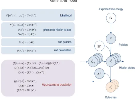
Figure 1: Generative model and (approximate) posterior. A generative model specifies the joint probability of outcomes or consequences and their (latent or hidden) causes. Usually the model is expressed in terms of a likelihood (the probability of consequences given causes) and priors over causes. When a prior depends on a random variable, it is called anempirical prior. Here, the likeli-hood is specified by a high-dimensional array Awhose components are the probability of an outcome under every combination of hidden states. The em-pirical priors in this instance pertain to transitions among hidden statesBthat may depend on action, where actions are determined probabilistically in terms of policies (sequences of actions denoted byπ). The key aspect of this genera-tive model is that policies are more probable a priori if they minimize the (path integral of) expected free energyG. Bayesian model inversion refers to the in-verse mapping from consequences to causes—estimating the hidden states and other variables that cause outcomes. In variational Bayesian inversion, one has to specify the form of an approximate posterior distribution, which is provided in the lower panel. This particular form uses a mean-field approximation in which posterior beliefs are approximated by the product of marginal distribu-tions over hidden states or factors. Here, a mean-field approximation is applied both to posterior beliefs at different points in time and factors. (See the appendix and Table 2 for a detailed explanation of the variables.) The Bayesian network (right panel) provides a graphical representation of the dependencies implied by the equations on the left. Here (and in subsequent figures),t denotes the current time point, andτindexes all possible time points.

(11)

Figure 2: Schematic overview of belief updating. The left panel lists the belief updates mediating perception (i.e., state estimation), policy selection, and learn-ing; while the right panel assigns the updates to various brain areas. This attri-bution is purely schematic and serves to illustrate a crude functional anatomy. Here, we have assigned observed outcomes to visual representations in the oc-cipital cortex, with visual (what) modalities entering a ventral stream and pro-prioceptive (where) modalities originating a dorsal stream. Auditory feedback is associated with the auditory cortex. Hidden states encoding context have been associated with the hippocampal formation and association (parietal) cortex. The evaluation of policies, in terms of their (expected) free energy, has been placed in the caudate. Expectations about policies, assigned to the putamen, are used to create Bayesian model averages of future outcomes (e.g., in the frontal eye fields and supplementary motor area). Finally, expected policies specify the most likely action (e.g., via the deep layers of the superior colliculus). The ar-rows denote message passing among the sufficient statistics of each factor or marginal. The appendix and Table 2 explain the equations and variables.

states and outcomes has been observed. In this article, we focus on learning the likelihood model and therefore assume that state transitions and initial states are known (or have been learned).

The generative model in Figure 1 means that outcomes are generated in the following way. First, a policy is selected using a softmax function of the expected free energy for each policy. Sequences of hidden states are generated using the probability transitions specified by the selected pol-icy. Finally, these hidden states generate outcomes in one or more modali-ties. Figure 2 (left panel) provides a graphical summary of the dependencies

(12)

implied by the generative model in Figure 1. Perception or inference about hidden states (i.e., state estimation) corresponds to inverting a generative model given a sequence of outcomes, while learning corresponds to up-dating the parameters of the model. Perception therefore corresponds to optimizing expectations of hidden states and policies with respect to vari-ational free energy, while learning corresponds to accumulating concentra-tion parameters. These constitute the sufficient statistics of posterior beliefs, usually denoted by the probability distributionQ(x), wherex=s˜, π,Aare hidden or unknown quantities.

2.2 Variational Free Energy and Inference. In variational Bayesian in-ference, model inversion entails minimizing variational free energy with respect to the sufficient statistics of approximate posterior beliefs. These be-liefs are approximate because they assume the posterior can be factorized into marginal distributions—here, over hidden states at each point in time, policies, and parameters. This is known as a mean-field assumption (see the factorization of the approximate posterior in the lower right panel of Figure 1). The ensuing minimization of free energy with respect to posterior beliefs can be expressed as follows (see Table 2 for a glossary of expressions):

Q(x)=arg min Q(x)F ≈P(x|o)˜, F=EQ[lnQ(x)−lnP( õ,x)], =D[Q(x) ||P(x|o)]˜ divergence − lnP( õ) log evidence =D[Q(x) ||P(x)] complexity −EQ[lnP( õ|x)] accuracy , (2.1)

where ˜o=(o1, . . . ,ot) denotes observations up to the current time. Because

the (Kullback-Leibler, KL) divergence cannot be less than zero, the penulti-mate equality means that free energy is minimized when the approxipenulti-mate posterior is the true posterior. At this point, the free energy becomes the negative log evidence for the generative model (Beal, 2003). This means that minimizing free energy is equivalent to maximizing model evidence, which is equivalent to minimizing the complexity of accurate explanations for ob-served outcomes.

Minimizing free energy ensures expectations encode posterior beliefs, given observed outcomes. However, beliefs about policies rest on future outcomes. This means that policies should, a priori, minimize the free en-ergy expected in the future (Friston et al., 2015). This can be formalized as

(13)

(negative)intrinsic or epistemicvalue

− EQ˜[lnP(oτ)]

extrinsic or expectedvalue =E_Q˜[lnQ(A)−lnQ(A|sτ,oτ, π)] ignorance +D[Q(o τ|π)||P(oτ)] risk + EQ˜[H[P(oτ|sτ)]] ambiguity (2.2)

where ˜Q=Q(oτ,sτ|π)=P(oτ|sτ)Q(sτ|π) is the posterior predictive

distri-bution over hidden states and their outcomes under a particular policy. When comparing the penultimate expressions for expected free energy (see equation 2.2) with the free energy per se (see equation 2.1), one sees that the expected divergence becomes mutual information or information gain (see the appendix). Here, we have associated the information gain about the parameters with novelty and information gain about hidden states with in-trinsic or epistemic value (i.e., salience). Similarly, expected log evidence becomes expected or extrinsic value provided we associate the prior pref-erence (log probability) over future outcomes with value. The last equality provides a complementary interpretation in which the expected complex-ity of parameters and hidden states becomes ignorance and risk, while expected inaccuracy becomes ambiguity. We have chosen to label inverse novelty as ignorance in the sense that novelty affords the opportunity to re-solve ignorance (i.e., nescience), namely, uncertainty about the contingen-cies that underwrite outcomes.

There are several special cases of expected free energy that appeal to (and contextualize) established constructs. For example, maximizing mu-tual information is equivalent to maximizing (expected) Bayesian surprise (Itti & Baldi, 2009), where Bayesian surprise is the divergence between pos-terior and prior beliefs. This can also be interpreted in terms of the principle of maximum mutual information or minimum redundancy (Barlow, 1961; Linsker, 1990; Olshausen & Field, 1996; Laughlin, 2001). Because mutual information cannot be less than zero, it disappears when the (predictive) posterior ceases to be informed by new observations. This means epistemic

(14)

behavior will search out observations that resolve uncertainty about the state of the world (e.g., foraging to resolve uncertainty about the hidden lo-cation of prey or fixating on an informative part of a face). However, when there is no posterior uncertainty, and the agent is confident about the state of the world, there can be no further information gain, and epistemic value will be the same for all policies, enabling extrinsic value to dominate (if it did not already). This resolution of uncertainty is closely related to satisfy-ing artificial curiosity (Schmidhuber, 1991; Still & Precup, 2012) and speaks to the value of information (Howard, 1966), particularly in the context of evincing information necessary to realize rewards or payoffs (see Meder & Nelson, 2012). (See also Nelson et al., 2010, who compare different models of information gain in explaining perceptual decisions.) Expected complexity or risk is exactly the same quantity minimized in risk-sensitive or KL con-trol (Klyubin, Polani, & Nehaniv, 2005; van den Broek, Wiegerinck, & Kap-pen, 2010), and underpins related (free energy) formulations of bounded rationality based on complexity costs (Braun, Ortega, Theodorou, & Schaal, 2011; Ortega & Braun, 2013). In other words, minimizing expected complex-ity renders behavior risk sensitive, while maximizing expected accuracy in-duces ambiguity-resolving behavior.

The new term introduced by this article is the information gain pertain-ing to the likelihood mapppertain-ing between hidden states and outcomes. This term means that policies will be more likely if they resolve uncertainty— not about hidden states – but about how hidden states generate outcomes. Put simply, this means policies that expose the agent to novel combinations of hidden states and outcomes become attractive because they provide ev-idence for the way that outcomes are generated. In other words, policies that afford a high degree of novelty resolve ignorance about the relationship between causes and consequences. The subsequent resolution of this igno-rance or uncertainty lends meaning to outcomes (consequences) in terms of hidden states (causes). This epistemic affordance will be important in what follows.

2.3 Belief Updating. Having defined our objective function, the suf-ficient statistics encoding posterior beliefs can be updated by minimizing variational free energy. Figure 2 provides these updates. Although the up-dates look complicated, they are remarkably plausible in terms of neurobio-logical schemes, as discussed in Friston et al. (2014) and Friston, FitzGerald et al., 2016). The update rules for expected policies (policy selection) and learning are the solutions that minimize free energy, while the updates for expectations over hidden states (for each policy and time) are formulated as a gradient descent. This is important because it provides a dynamical pro-cess theory that can be tested against empirical measures of neuronal dy-namics. We will see examples of simulated neuronal responses later. Note that the solution for expected policies is a classical softmax function of ex-pected free energy, while learning entails accumulation of concentration

(15)

parameters based on the co-occurrence of outcomes and combinations of expected hidden states. Here, the expected hidden states constitute Bayesian model averages over policy-specific expectations (See Friston, FitzGerald et al., 2016) for a more thorough discussion of the neurophys-iological implementation of these updates.)

In novel environments, the heavy lifting rests on learning the parame-ters (and form) of the likelihood mapping. The interesting aspect of these parameters is that they mediate interactions among different hidden states. In other words, they play the role of connections from hidden states to pre-dicted outcomes. From a neurobiological perspective, this means that the connections generating predicted outcomes from expected states (or up-dating hidden states based on outcomes) are necessarily activity dependent and context sensitive. For example, the first term in the expression for state estimation or perception in Figure 2 is a linear mixture of outcomes formed by a connectivity matrix that itself depends on expectations of over hid-den states. In other words, hidhid-den states interact or conspire to generate predictions—or select mixtures of outcomes for Bayesian belief updating. We will return to the importance of these interactions when we consider structure learning.

2.4 Summary. By assuming a generic (Markovian) form for the genera-tive model, it is straightforward to derive Bayesian updates that clarify the interrelationships among perception, planning (i.e., policy selection), and learning. In brief, the agent first infers the hidden states under each policy that it entertains. It then evaluates the evidence for each policy based on observed outcomes and beliefs about future states. Posterior beliefs about each policy are then used to select the next action. The ensuing outcomes are used in conjunction with combinations of expected hidden states to ac-cumulate experience and learn contingencies or model parameters. Figure 2 (right) shows the functional anatomy implied by the belief updating and mean-field approximation in Figure 1. Table 1 lists the sources of uncer-tainty encoded by (expected) variational free energy and the behaviors en-tailed by its minimization. As noted in section 1, this formalism provides a nice ontology for perception, planning, and learning where planning or policy selection has distinct novelty, information, and goal-seeking com-ponents (driven by novelty, salience, and extrinsic value, respectively). We will use this formalism in the next section to illustrate the behavioral (and electrophysiological) responses that attend rule learning.

3 Curiosity and Learning

The first question is why human beings devote so much time and effort to the acquisition of knowledge (Berlyne, 1954).

(16)

The (rule-learning) paradigm considered in this section is sufficiently difficult to challenge audiences but simple enough for us to unpack for-mally. Its agenda is to illustrate curiosity in terms of pursuing policies that afford novelty and the epistemic learning that ensues. The paradigm in-volves three input modalities (what,where, andfeedback) and four sets of hidden states that generate these outcomes—two encoding contextual fac-tors (ruleandcolor) and two hidden states that can be controlled (whereand choice; see Figure 3).

In brief, artificial subjects could fixate or attend to a fixation point or one of three cue locations. They were told that the color of the central cue spec-ified a rule that would enable them to report the correct color (red,green, or blue) with a button press (red,green,blue, orundecided). They were told to report the correct color as accurately as possible after looking at three cues or fewer. The rule the subjects had to discover was as follows: the color of the central cue specifies the location of the correct color. For example, if the subject sees red in the center, the correct color is on the left. When demon-strating this task to audiences we usually say something like:

On each trial, we will present three colored dots, arranged around a cen-tral fixation point. Your task is to choose the correct color. The dots will be red, blue, or green, and dots of the same color can appear together. All we will tell you is that there is a rule that enables you to identify the cor-rect color on every trial—and that this rule is indicated by the color of the central dot. To make things interesting, you can see only one dot at a time, and we expect a decision after you have looked at three dots. Here is the first trial, which color do you think is correct?

Clearly, we did not instruct our synthetic subject verbally. These instruc-tions were conveyed via prior beliefs about the likelihood of outcomes and prior preferences over a feedback modality. These prior preferences ensured that the subject believed that she was unlikely to be wrong and that she was highly likely to decide after the third epoch (i.e., she was likely to comply with task instructions, even if this entailed choosing the wrong color). These prior beliefs were coded in terms of negative value (i.e., Cost) in a feedback modality;m=3, with three levels (undecided, right, and wrong):

Cm_τ = −lnP(om_τ)= ⎧ ⎪ ⎪ ⎨ ⎪ ⎪ ⎩ 4 om τ =wrong:∀τ >0,m=3 8 om τ =undecided:∀τ >3,m=3 0 otherwise (3.1)

In addition to the (visual)colorand (auditory)feedbackmodalities, subjects also received a (proprioceptive) feedback signalingwherethey were cur-rently looking. Here,τindicates the number of saccades or sampled cues in each trial.

(17)

The hidden state space induced by the above instructions has four fac-tors: the subject knew that there were three rules; three correct colors (red, green, or blue); where they were looking (left, center, right, or fixation); and their choice (red, green, blue, or undecided). We equipped subjects with six actions: they could look at (or attend to) any of the cue locations without making a choice, or they could return to the fixation point and report their chosen color. In these simulations, policies were very simple and comprised the past sequence of actions plus one of the six actions above. (See Figure 3 for a schematic depiction of the implicit hidden state space.)

The transition matrices were also simple. The first two are identity matri-ces, because the context (rule and color) states do not change within a trial. In what follows, each trial begins with a new set of cues and comprises a sequence of epochs, where an epoch corresponds to the belief updating fol-lowing each new observation (e.g., saccadic eye movement). The remaining (where and choice) probability transition matrices depend on action, where the action invariably changes the hidden state to where the subject looks or the choice she makes:

B1_{i j},2(u)= 1 i= j,∀u 0 i= j,∀u. B3_{i j},4(u)= 1 i=u,∀j 0 i=u,∀j. (3.2)

Finally, prior beliefs about the initial states were uniform distributions apart from the sampled location and choice, which was always looking at the fixation point prior to making a choiceDn₌_[0_{, . . . ,}₀_,_1].

The only outstanding parameters of the generative model are the con-centration parameters of the likelihood Am _{that link hidden states and}

outcomes. The agent effectively knew the mapping towhereandfeedback outcomes, in the sense that we made the concentration parameters high for the correct contingencies (with a value of 128) and zero elsewhere. In other words, the agents knew that feedback depended on choosing the correct color. Furthermore, we used informative concentration parameters to tell the subject that each of the three rules determined the color of the central cue. However, the agents did not know how the rule determined outcomes. This ignorance corresponds to uniform concentration parameters (of one) in the mapping between the correct color and the color seen at each loca-tion, under all three levels of the rule. The important parts of the resulting likelihood array are shown in Figure 3 (right inset panel). Here, we have tiled matrices mapping from the correct color (red, green, blue) to the vi-sual outcome (red, green, blue, gray) for each location sampled (columns) and rule (rows). This arrangement reveals the contingencies generating out-comes. For example, if the agent is looking at the central location, she will see a unique color under each rule (middle column: red, green, and blue for

(18)

each of the three rules). Although the color sampled at the central location signifies the rule for this trial, the subject has no concept of what this rule means (see the uniform priors on either side of the central fixation in Fig-ure 3). This means that the subject believes, a priori, there is no relationship between the correct color and the color observed.

This completes our specification of the subject’s generative model. An important aspect of this formulation is that we were able to transcribe task instructions or intentional set into prior beliefs. This suggests that one can regard task instructions as a way of inducing prior beliefs in an experimen-tal setting. After instilling these prior beliefs, the synthetic subject knows quite a lot about the structure of the problem but nothing about its so-lution. In other words, she knows the number of hidden states and their levels and mappings between some hidden states and others. However, this knowledge is not sufficient to avoid surprising outcomes: making mis-takes. Notice that we have been able to specify a fairly complete model of a paradigm, including where subjects look, when they expect to respond, and the sensory modalities entailed. This may appear to be overkill; how-ever, it allows us to make specific predictions about behavior that can be tested empirically. Furthermore, it shows how purposeful, epistemic behav-ior can emerge under minimal assumptions. In what follows, we will see abstract problem solving and rule learning emerge from the minimization

(19)

of expected free energy (i.e., expected surprise or uncertainty) under prior beliefs that make indecisive or erroneous choices surprising.

3.1 The Rule. Hitherto, we have just specified the generative model used by an agent. Clearly, to generate outcomes, we have to specify the true generative process. This is identical to the generative model with one exception: the mapping from states to outcomes contains the causal struc-ture or rule that the subject will learn. As noted, the actual rule used to generate outcomes is as follows: the rule (left, center, right) specifies the lo-cation of the correct color. For example, if the subject sees red in the center, the correct color is on the left. However, if she sees green in the center, the correct color is in the center, which is always green. The corresponding part

Figure 3: Graphical representation of the generative model (Left) The Bayesian network shows the conditional dependencies implied by the generative model in Figure 1. The variables in open circles constitute (hyper) priors, while the blue circles contain random variables. This format shows how outcomes are generated from hidden states that evolve according to probabilistic transitions, which depend on policies. The probability of a particular policy being selected depends on its expected free energy. The left panels show the particular hidden states and outcome modalities used to model rule learning. Here, there are three output modalities comprising colored visual cues (what), proprioceptive cues signaling the direction of gaze (where), and (auditory) cues providing feedback (feedback). These three sorts of outcomes are generated by the interactions among four hidden states or factors: an abstract rule indicating the location of an infor-mative color cue (rule); the correct color (colour), where attention or saccadic eye movements are directed (where); and a (manual) response (choice). Hidden states interact to specify outcomes in each modality. In other words, each combination of hidden states has an associated column in the likelihood array that specifies the relative likelihood of outcomes in each modality. For example, if the rule is left, the correctcoloris red, and the subject is looking at the left cue, thewhat outcome will beredand thewhereoutcome will beleft. (Right) The panel on the upper right shows an example of a trial, where a subject looks from the starting position to the central location, sees a red cue, and subsequently looks to the left. After she has seen a green cue, she knows the correct color and returns to the start position, while indicating her choice (green). The “?” denotes an undecided choice state (and feedback). The matrices (lower left panel) show the likelihood mapping between hidden states and (color) outcomes assumed, a priori, (right) and used to generate actual outcomes (left). These matrices show the likelihood mapping from hidden states towhatoutcomes—theAarray for the first orwhat modality. This is a five-dimensional array, of which four dimensions are shown under theundecidedlevel of thechoicefactor. In other words, these are the contin-gencies in play until a decision is made. These parameters are shown as a block matrix with 3×3 blocks (ruletimeswhere). Each block shows the 4×3 matrix mapping the correct color to the outcome. (See Figure 7 for further details.)

(20)

of the likelihood mapping (under the undecided state) is shown in Figure 3 (left inset panel). In contrast to the prior beliefs, the true likelihoods mean that if one is looking to the left, the observed color maps to the correct color under the left rule, and similarly when looking to the right. This true like-lihood also contains some redundancy. For example, if the subject looks at the central cue when the correct color is red, she will still see a green cue. However, this combination of hidden states never occurs because, a posteri-ori, a central green cue means the correct color is green (and this is encoded in the likelihood mapping under decided states). It should be noted that the (synthetic) subject does not “know” about these contingencies in an ex-plicit or even subpersonal sense. These contingencies are encoded in model (concentration) parameters that can be associated with synaptic efficacy or connection strengths in the brain.

The rule above may sound simple, but it introduces interesting context sensitivity or interactions among the hidden factors causing outcomes. For example, the outcome depends on a two-way interaction between the cor-rect color and where the subject is looking, but only when the rule is right or left. The subject has to learn these contingencies by accumulating co-incidences of inferred states and outcomes. However, this is not a simple problem because agents do not have complete knowledge about hidden states and therefore do not know which states are responsible for generat-ing outcomes. Imagine you had to identify these interactions by designgenerat-ing a multifactorial experiment. You would then manipulate hidden states and record the outcomes. However, there is a problem: you do not know the hidden states (because they are hidden from direct observation). In other words, our synthetic subject has to learn the parameters, while inferring the hidden states. So how does she fare using active inference?

Figure 4 shows the results of simulating 32 trials, where each trial com-prises six epochs in which the subject can sample a new cue or make a choice. The upper two panels summarize performance in terms of poste-rior expectations over policies (top panel) and the final outcomes (second panel). The colored dots indicate the rule for each trial (upper panel) and the final outcomes (second panel). A key point to observe is that the final out-come is usually correct. This is because the subject is allowed to change her mind after making a mistake. These choices are based on posterior expecta-tions about policies that are initially ambiguous and become more precise with learning. By the end of each trial, only the last three policies are tained (choosing red, green, or blue). In the first trial, two options are enter-tained with equal probability, but by the 10th trial, any ambiguity appears to be resolved. After the 14th trial, performance becomes perfect. Although there is no definitive phase transition or aha moment, these results suggest that the rule is dawning on the agent.

The lower panels illustrate the implicit transition from ignorance to un-derstanding after trial 14 (highlighted in blue). The second and third panels

(21)

Figure 4: Simulated responses during learning. This figure reports the behav-ioral responses during 32 successive trials. The first panel shows the first (rule) hidden state as colored circles and subsequent policy selection (in image format) over the policies considered. Darker means more probable. There are six poli-cies corresponding to a saccade to each of the three locations (without making a choice) and three choices (while moving back to the starting location). These policy expectations reflect the fact that at the end of the trial, a choice is always made with greater or lesser confidence, as reflected in the relative probability of the final three policies. The second panel reports the final outcomes (encoded by colored circles) and performance measures in terms of expected cost (see equation 3.1 and Table 1), summed over time (black bars). The red bars indicate mistakes (i.e., the incorrect color is chosen at some point).The lower two panels report the free energy at the end of each trial and fluctuations in confidence as learning proceeds. The cyan region indicates the onset of confident and correct responses.

(22)

show the free energy over trials and associated confidence in behavior:π·π (i.e., the negative entropy of beliefs about policies, where entropy scores uncertainty). Note that free energy is the difference between accuracy and complexity. The increase in confidence therefore reflects a dialectic between complexity and accuracy. Here, the increase in confidence (decrease in en-tropy over policies) is more than offset by the increase in accuracy afforded by confident behavior. This is reflected by the progressive decrease in free energy that, unlike confidence, shows trial-to-trial fluctuations. The persis-tent increase in confidence is underwritten by epistemic behavior that re-solves both uncertainty and ambiguity.

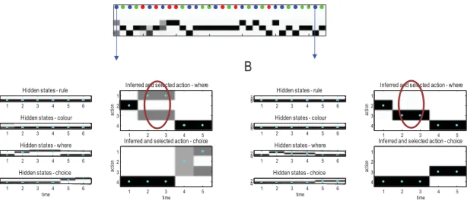
Figure 5 shows the expectations over states and action as a function of epochs within the first trial (see Figure 5A) and the penultimate trial, after rule learning (see Figure 5B). The four panels on the left show the expec-tations over the four marginal hidden states, while the two panels on the right show the equivalent expectations over action. Note that there are two actions that control transitions among hidden states: thewherefactor and thechoicefactor. The cyan dots show the true hidden states and action se-lected. In the first trial, the agent first looks to the center, then looks to the left, stays there for one epoch, and then makes two incorrect choices. Con-versely, in the later trial, the agent looks at the center, and the right and then chooses correctly.

The key point these results illustrate is the apparent attractiveness of right and left locations after the first saccade, which disappears in later tri-als. It is this behavior that is driven by novelty (see equation 2.2). To under-stand the importance of this behavior, it is useful to realize that the right and left locations are inherently aversive because they deliver ambiguous out-comes. Normally, an agent would avoid these locations in the same way that you and I might avoid a noisy restaurant or ambiguous invitation. How-ever, the naive agent does not know these locations are ambiguous—and this is a known unknown that affords an opportunity for the agent to fill in her knowledge gaps. Crucially, after rule learning, the subject knows that the left location is ambiguous and avoids it (compare the probabilities in the upper right panels in Figures 5A and 5B). She therefore looks immedi-ately to the informative location, enabling her to retrospectively infer that the correct color is blue (compare the upper left panels in Figures 5A and 5B). This inference is based on Bayesian belief updating, which we now consider more closely.

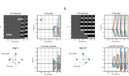
3.2 The Neural Correlates of Cognizance. A close inspection of the (synthetic) neuronal updating—underwriting the behavior above—shows a profound difference in the temporal structure of evoked responses. Fig-ure 6 shows the activity of units encoding the expectation of the hidden color state over six epochs as a function of time. The results are shown for the same (before and after learning) trials of the previous figure. The upper

(23)

Figure 5: Simulated exploration. This figure reports the belief updating behind the behavior shown in Figure 4 for an early trial (A) and after the rule has been learned (B). (A) Each panel shows expectations in image format, with black representing 100% probability. For the hidden states (left panels), each of the four factors is shown separately, with the true states indicated by cyan dots. Here, there are five saccades, and expectations are shown after completion of the last saccadic, which means that, retrospectively, the agent believes it started in a right rule context (hidden states—rule) and, despite making two mistakes, is able to infer the correct color by elimination (hidden states—color). The two panels on the right report the equivalent expectations about action for the two controllable hidden states (whereand choice). The sequence of sampling (in-ferred and selected action—where) indicates that the subject first interrogated the center (observing a blue cue), looked to the left, and then made two incorrect choices (see Figure 6). (B) However, after learning, the subject is much more con-fident about where to look because she now knows that the color of the right cue will reduce uncertainty about the correct color. The important aspect of these re-sults is that prior to learning, the right and left locations are equally attractive— and more attractive than the (initially sampled) central location (highlighted with red circles). This is despite the fact these locations do not reduce risk or uncertainty (because the agent does not know the meaning of the cues in these locations). However, the subject does know that she is ignorant and can resolve this ignorance by exposing herself to novel outcomes.

panels show belief updates as a raster image (left) and as functions of peri-stimulus time (right). The raster highlights the fact that there are explicit representations of the six epochs at each point in time and that these expec-tations are updated over time. This means that the blocks of the raster above the leading diagonal encode the past, while the blocks below the leading di-agonal encode the future.

The key observation here is that the onset of discriminatory responses is much earlier after learning than before. This is due to—and only to— learning the mapping between hidden states and consequences, enabling

(24)

Figure 6: Simulated electrophysiological responses. This figure shows expec-tations about hidden states for the same two trials illustrated in the previous figure—before learning (A) and after learning (B). (A) The upper left panel shows the activity (firing rate) of units encoding the correct color in image (raster) format over the six intervals between five saccades. These responses are organized such that the upper rows encode the probability of alternative states in the first epoch, with subsequent epochs in lower rows. In other words, the top row shows the expectations about the three hidden (color) states at the beginning of the trial and how these expectations evolve over time. Conversely, the first column shows expectations about the three colors at successive time points in the future. The plot to the right of the image presents the same infor-mation to illustrate the evidence accumulation and the resulting disambigua-tion of context. These values are expectadisambigua-tions about hidden states described by the first equations in Figure 2 and can be interpreted as neuronal firing rates of units encoding expectations. The associated local field potentials for these units (i.e., the rate of change of neuronal firing) are shown in the lower plot. The in-sert (lower left) shows the sequence of moves and decisions. Here, the subject makes a saccade to the center location and then looks to the left and finally back to the center, at which point she makes a choice (green), which elicits the wrong feedback. She then changes her mind and (incorrectly) tries red. However, the correct color is blue (circled in magenta). This behavior can be contrasted with the responses on the right (after learning). (B) Here, the correct color is identi-fied on the first choice. Crucially, this is based on precise expectations about the correct color that have been accumulating since the second saccade, as reflected in the simulated neuronal responses.

the agent to infer the correct color after the second saccade to the (infor-mative) location. The lower panels show the corresponding behaviors (left) and simulated local field potentials or event-related potentials (right). These are simply the first derivatives of the responses in the upper panels. In

(25)

summary, after the rule has dawned on the agent, she knows exactly where to find unambiguous information to make precise inferences about the un-derlying context and veridical choices. In terms of simulated electrophysi-ology, this means representations of latent states of the world are activated much earlier during evidence accumulation, after the meaning of cues has been disambiguated through epistemic learning. These simulations are not inconsistent with event-related potential and fMRI studies of insight, re-viewed in the discussion (e.g., Jung-Beeman et al., 2004; Mai, Luo, Wu, & Luo, 2004; Bowden et al., 2005).

4 Structure Learning and Bayesian Model Reduction

The second question is why, out of the infinite range of knowable items in the universe, certain pieces of knowledge are more ardently sought and more readily retained than others (Berlyne, 1954).

The previous section illustrated the role of novelty in driving curious be-havior and the epistemic learning it elicits. In this section, we turn to a different sort of learning: learning the structure of a likelihood model af-ter evidence has been accumulated. The previous simulations suggest that there are behavioral and electrophysiological correlates of curiosity in epis-temic learning. However, there was no clear homologue of an aha moment or an instance of revelation associated with insight. To move closer to ”the perception of what passes in a man’s own mind,” this section considers Bayesian model selection and structure learning as a metaphor of under-standing and self-knowledge, in the sense of Locke (Nimbalkar, 2011). It considers the fact that subjects not only have prior beliefs about the param-eters of their models but also prior beliefs about models per se; for exam-ple, they know there are rules. In what follows, we will see that this prior knowledge about models naturally induces abductive reasoning, when the models themselves minimize variational free energy.

Loosely speaking, one can associate awareness of the world with infer-ence about its hidden states based on a generative model and knowledge with learning model parameters. Here, we turn to a third level of optimiza-tion that minimizes free energy with respect to the model per se. Select-ing models that have the greatest evidence (least free energy) is known as Bayesian model selection. This procedure furnishes models that, on aver-age, provide the best explanation for the data at hand. As such, it can be thought of as inference to the best explanation (Harman, 1965), or abduc-tive reasoning.

We focus on a particular but ubiquitous form of Bayesian model selec-tion; Bayesian model reduction. Essentially, Bayesian model reduction eval-uates the evidence of reduced forms of a parent or full model by eliminating redundant parameters. Crucially, Bayesian model reduction can be applied to the posterior beliefs after the data have been assimilated. In other words,

(26)

Bayesian model reduction is a post hoc optimization that refines current beliefs based on alternative models that may provide potentially simpler explanations (Friston & Penny, 2011). The alternative (reduced) models are defined in terms of their priors—for example, a precise prior belief that some parameters are zero. Heuristically, equation 2.1 shows that free en-ergy is a complexity minus accuracy, where complexity is the divergence between posterior and prior beliefs. Previously, we have focused on opti-mizing free energy with respect to the (approximate) posterior as encoded by its expectations. However, we can also minimize free energy with respect to the priors, thereby eliminating redundant parameters to reduce model complexity.

Neurobiologically, this model optimization resembles mechanisms that have been proposed during sleep. While awake, the brain learns causal associations, through associative plasticity, that are embodied in an exu-berance of synaptic connections. During sleep, redundant connections are subsequently removed (Tononi & Cirelli, 2006) to minimize complexity and free energy in the absence of any further sensory input (Hobson & Friston, 2012). In this setting, sleeping is literally a way of clearing one’s mind.

Technically, Bayesian model reduction is a generalization of ubiquitous procedures in statistics, ranging from the Savage-Dickey ratio (Savage, 1954), through to classicalF-tests in parametric statistics. In our context, it reduces to something remarkably simple: by applying Bayes’ rules to full and reduced models, it is straightforward to show that the change in free energy can be expressed in terms of posterior concentration parametersa, prior concentration parametersa, and the prior concentration parameters that define a reduced or simpler model a’. Using B(·) to denote the beta function, we get (see the appendix)

F=ln B(a)+ln B(a)−ln B(a)−ln B(a+a−a). (4.1)

This equation returns the difference in free energy we would have observed had we started observing outcomes with simpler prior beliefs. Clearly, to engage with this form of free energy minimization, one has to have a space of models or reduced priors to evaluate. This is the key feature of Bayesian model reduction that lends it an abductive aspect: in other words, model se-lection is ampliative, meaning that the conclusion goes beyond what could otherwise be induced or inferred. This abductive characteristic rests on the selection of competing hypotheses that are plausible. In other words, if I know that my data were produced like this or like that, I can appeal to a relatively small number of plausible explanations and implicitly exclude a universe of alternative explanations (models), including the full model used to acquire my knowledge. This ampliative aspect of Bayesian model selection appeals to a hierarchical structuring of plausible explanations such that each successive level provides broad (or abstract) constraints on

(27)

plausible explanations for the level below; for example, at the highest level, we may know there are a small number of plausible hypotheses and a large number of implausible hypotheses. (See Navarro & Perfors, 2011, for a discussion of this key issue in the context of sparse hypothesis or model spaces.)

To make this process clear, consider the following example. If our subject knows she is being asked to discover a rule, she knows that some combina-tions of hidden states for each factor will be informative and others will not. Therefore, under any particular combination of hidden states, there are only two plausible contingencies: either all allowable outcomes are equally prob-able, or there is a definitive outcome that constitutes part of the rule. One can take this explanatory reduction (of model or hypothesis space) even further based simply on the assumption that rules entail some form of symmetry or invariance. For example, if the correct color red always generates a red outcome, other levels of the same (color) hidden state will be informative under a particular combination of the other hidden states.

This heuristic can be absorbed gracefully into the imperative to minimize expected free energy. This is because expected free energy scores the ambi-guity of a generative model. Therefore, prior beliefs about models based on their expected free energy will necessarily favor unambiguous map-pings between (latent) causes and consequences. In other words, in exactly the same way that action selection minimizes ambiguity, when agents are equipped with the latitude to optimize their models, model selection is re-stricted to models whose plausibility is determined by their ability to dis-ambiguate the causes of observed outcomes.

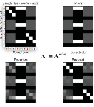
Figure 7 shows the results of applying Bayesian model reduction before the 12th trial in the simulations above. In this example, we compared the evidence for a full model (in which the correct color generated outcome colors of equal probability) with reduced models in which the correct color generated its own color (under each combination of the remaining hidden states). These reduced models were specified by changing the prior counts from 1 to 8 to specify a prior belief that the hidden color specified the out-come more precisely. A comparison was performed under every combina-tion of the remaining (three) hidden states. If there was positive evidence for the reduced, simpler, or unambiguous model, the concentration param-eters mediating uninformative outcomes were removed (by setting them to zero) and the posterior concentration parameters (or counts) were assigned to the remaining parameters.

The upper left panel of Figure 7 reproduces the true likelihood from Figure 3. The upper right panel shows the full model that corresponds to the agent’s prior beliefs. The equivalent posterior beliefs after 12 trials are shown on the lower left. It is clear that the leading diagonal blocks of the array may be better explained by an unambiguous one-to-one map-ping between the hidden and outcome colors. Indeed, when we performed Bayesian model comparison, the reduced model had more evidence than