Ramp metering and freeway bottleneck capacity

Ramp metering and freeway bottleneck capacity

Lei Zhang

_{, David Levinson}

a_{Department of Civil and Environmental Engineering, University of Maryland, 1173 Glenn Martin Hall, College Park, MD 20742, United States}

b_{Department of Civil Engineering, University of Minnesota, 122 Civil Engineering Building, 500 Pillsbury Drive SE, Minneapolis, MN 55455, United States}

a r t i c l e i n f o Article history:

Received 20 January 2009

Received in revised form 8 January 2010 Accepted 16 January 2010

Keywords: Ramp metering Highway capacity Active bottleneck Queue discharge flow

Twin Cities ramp meter shut-off

a b s t r a c t

This study aims to determine whether ramp meters increase the capacity of active freeway bottlenecks. The traffic flow characteristics at 27 active bottlenecks in the Twin Cities have been studied for seven weeks without ramp metering and seven weeks with ramp meter-ing. A methodology for systematically identifying active freeway bottlenecks in a metro-politan area is proposed, which relies on two occupancy threshold values and is compared to an established diagnostic method – transformed cumulative count curves. A series of hypotheses regarding the relationships between ramp metering and the capac-ity of active bottlenecks are developed and tested against empirical traffic data. It is found that meters increase the bottleneck capacity by postponing and sometimes eliminating bottleneck activations, accommodating higher flows during the pre-queue transition per-iod, and increasing queue discharge flow rates after breakdown. Results also suggest that flow drops after breakdown and the percentage flow drops at various bottlenecks follow a normal distribution. The implications of these findings on the design of efficient ramp control strategies, as well as future research directions, are discussed.

!2010 Elsevier Ltd. All rights reserved.

1. Introduction

Ramp metering, since its debut in the early 1960s (May, 1964), has been widely deployed in many urban areas. Meters can reduce average freeway commuter delay by appropriately managing entrance ramp inflows. Other positive impacts of ramp metering, such as improved safety, more reliable travel time, reduced emission and fuel consumption, and high occu-pancy vehicle (HOV) priority, traffic diversion to under-utilized local streets, have also been reported in past studies (e.g.

Zhang,2007; Levinson and Zhang, 2006; Cambridge Systematics, 2001), but are often considered as secondary objectives even though their benefits may exceed the reduction in travel delay. When designing ramp metering algorithms, engineers and researchers usually focus on the improvement of freeway mainline capacity. However, the fundamental relationship be-tween ramp metering and freeway capacity has not been adequately studied. The important question of whether ramp metering increases the capacity at freeway bottlenecks has not found a conclusive answer. A better understanding of this issue would generate information valuable to both researchers and practitioners, such as control threshold values (i.e. the optimal volume or density used as control objectives) in local or coordinated ramp metering algorithms.

Active bottlenecks are characterized by queue discharge flows not affected by traffic conditions further downstream (Daganzo, 1997). Several studies, by carefully examining traffic data before and after breakdown at active bottlenecks, reveal that maximum flow rates diminish after queues form upstream (Cassidy and Bertini, 1999; Hall and Agyemang-Duah, 1991; Banks, 1991a,b). The two-capacity hypothesis argues that metering can increase bottleneck capacity by preventing, or at

0965-8564/$ - see front matter!2010 Elsevier Ltd. All rights reserved. doi:10.1016/j.tra.2010.01.004

*Corresponding author. Tel.: +1 612 625 6354; fax: +1 612 626 7750. E-mail addresses:[email protected](L. Zhang),[email protected](D. Levinson). 1 _{Tel.: +1 301 405 2881; fax: +1 301 405 2585.}

Contents lists available atScienceDirect

Transportation Research Part A

least postponing queue formation on the freeway mainline (Banks, 1990). Several simulation studies with simplified demand patterns on hypothetical networks provide evidence that ramp metering can increase bottleneck flows in a simulated envi-ronment (Persaud et al., 2001; Kotsialos et al., 2002). Whether it is also true in reality is not clear. The work ofCassidy and Rudjanakanoknad (2002)examines flow characteristics at one merging bottleneck with four days of metering-off and -on data. Their method with a focused local setup can provide detailed information for analysis of capacity-related issues at indi-vidual bottlenecks. It should be pointed out that some other studies suggest the two-capacity phenomenon does not provide a basis for ramp metering because the observed flow drop after breakdown seems insignificant (Newman, 1961; Persaud, 1986; Persaud and Hurdle, 1991).

The overall objective of this study is to determine whether ramp metering increases the capacity at freeway bottlenecks, and statistically test this hypothesis against a large empirical multi-bottleneck dataset. As suggested byBanks (1990), the most direct way to answer this question would be to experiment with metering rates, including turning the meters off. An-other approach is to document flow processes carefully in the vicinity of bottlenecks to determine the possible effects of metering. Most previous studies adopted the second approach, probably due to the lack of traffic data under different meter-ing status. The shortfall of this approach is that several important questions cannot be answered with metermeter-ing-on or -off traffic data alone. For instance, these studies cannot test whether the queue discharge flow rates with metering are signif-icantly higher than without metering. It is fortuitous for researchers that the Twin Cities ramp metering shut-off experiment occurred in 2000. The database constructed during the experiment allows us to examine more than 250 km of freeways for a long period of time with and without ramp metering. A detailed description of the background and the timeline of this shut down experiment can be found in previous studies (Levinson and Zhang, 2006; Zhang and Levinson, 2004a). Using this data set, we are able to statistically test several hypothesized relationships between ramp metering and freeway bottleneck capacity.

Before proceeding to the analysis, we would like to discuss several important concepts and terms regarding ramp meter-ing which will be referred to later in this paper. Such a discussion also helps readers understand the value and limitations of this work. First, increased capacity at bottlenecks is not a necessary condition for ramp metering to reduce commuter delay. The real necessary condition with fixed freeway demand is that ramp metering shifts the system departure curve in a man-ner such that the area bounded by the departure and arrival curves in the queuing diagram is narrowed. In terms of termi-nology, we reserve output for the departure rate of the whole freeway system (mainline plus ramps), and capacity for homogenous freeway sections. We follow the capacity definition ofZhang and Levinson (2004b), which states capacity at a bottleneck is a weighted sum of its pre-queue transition flow rate and queue discharge flow rate. Ramp metering increases freeway bottleneck capacity if it increases both pre-queue transition flow and queue discharge flow rates. Even if the capac-ity at bottlenecks does not increase with metering (we refer to capaccapac-ity increase at bottlenecks as aType II capacity increase hereafter in the paper), the flow on mainline sections and exit ramps upstream of bottlenecks may increase because ramp meters to some extent prevent queue formation and in case a queue has already formed, limit its physical length, so that fewer exit ramps are blocked and trips with destination off-ramps upstream of the bottleneck are either not delayed or de-layed less (aType I capacity increase). Therefore, totaloutputcan still be improved even though nothing changes at bottle-necks. This benefit of ramp metering was recently expounded byCassidy (2003). Therefore, reduced freeway travel time or delay does not necessarily provide evidence that ramp metering increases bottleneck capacity unless observed off-ramp flow increases are not sufficient by themselves to explain the travel time reduction. For the same reason, previous studies not explicitly considering active bottlenecks shed no light on the hypotheses tested in the present paper. It should also be noted that identifying the optimal control strategy is not the goal of this research, though some results from this empirical analysis may be used by future studies toward that goal. In that case, the impact of traffic waiting at meters must be considered.

Section2of this paper describes the study sites and traffic data in detail. Section3develops a series of statistically test-able hypotheses about the impacts of ramp metering on bottleneck capacity. For the purpose of this research, an appropriate data analysis tool is required to help identify active bottlenecks, queue discharge flows and other related traffic character-istics. Section 4 illustrates the occupancy method with two threshold values used in this study, followed by results of hypothesis testing in Section 5. The final section concludes the study and discusses the implications of the findings on the design of effective ramp control strategies.

2. Data and study sites

Seventy-five percent of the Twin Cities metro area freeways are served by a traffic management system including cam-eras, inductive loop detectors, ramp meters, variable message signs, and incident management. The Minnesota Department of Transportation (MnDOT) installed the first ramp meter on I-35E in 1969 in the Twin Cities metropolitan area. The ramp metering system has since grown to include 440 ramp meters with 235 operating during the morning peak period and 285 operating during the afternoon peak period by the time a bill passed in the 2000 Minnesota Legislature requiring a shut down experiment to study the effectiveness of the system. The experiment provided 32 flow and occupancy data from nearly 4000 single loop detectors during a seven-week period (from the third week of October to the first week of December in 2000) without ramp metering. Although loop detector data for the metering-on scenario are available for all days after instal-lation, only the corresponding seven weeks in 1999 were selected as the study period for the metering-on scenario for rea-sons explained later in this section. Raw traffic data (flow and occupancy) were extracted in 30-s intervals from MnDOT

archived binary data files which are available to the public (TDRL, 2004). Video data collected by surveillance cameras were, however, not archived for privacy concerns. Since it is impossible to validate detector data with video information, a com-prehensive detector error test was performed to ensure that data from corrupt detectors were not included in the analysis. Past studies (Chen and May, 1987; Jacobson et al., 1990) proposed various methods for identifying corrupt detectors, men-tioned eight types of detector failures, and suggested corresponding test algorithms (missing data, zero volume and occu-pancy, zero volume and 100% occuoccu-pancy, constant non-zero volume and occuoccu-pancy, zero volume but non-zero occupancy, non-zero volume but zero occupancy, practically impossible volume (>3600 veh/ln/h) or occupancy (>90%), bad flow conservation at adjacent detection stations (flow discrepancies >500 veh/lane/24 h)). These tests were performed on all raw traffic data used in this study and corrupt detectors were simply eliminated from the analysis. No efforts have been made to repair missing or suspicious data. More specifically, we wrote a Java program which reports detection malfunc-tioning information including start time, duration, and type of malfuncmalfunc-tioning. If any type of detection error lasted for more than two consecutive intervals in which traffic data might be used for the subsequent capacity analysis, the corresponding detector and the detection station will be considered as corrupt for the whole peak period.

In 1999, all studied freeways were controlled by the Minnesota zonal metering algorithm, a real-time, coordinated strat-egy that limits inflows at predetermined groups of on-ramps upstream of bottlenecks in order to keep bottleneck flows strictly below some flow threshold values (MnDOT, 1998;Bogenberger and May, 1999). The threshold values are usually around 2220 veh/lane/h based on historical data. Several occupancy threshold values are also established in the algorithm to detect queues. If the algorithm identifies that breakdown has already occurred and a queue is present (marked by high occupancy values upstream of the bottleneck), stricter metering rates will be applied in order to dissipate the mainline queue. This study focuses on the afternoon peak period (13:00–21:00). The earliest possible starting time and the latest pos-sible ending time of ramp metering operation during afternoon peak periods are 14:30 and 19:30 respectively. The study has also been restricted to normal weekdays so that the driving population is relatively constant and familiar with the facilities. The Thanksgiving holidays are omitted.

Besides the metering status, weather conditions, demand fluctuation, accidents, and road maintenance activities all have significant impacts on measured flow and occupancy values, and can potentially bias hypothesis testing results. Therefore, we developed and implemented a data filter in order to appropriately control for those factors. Weather data were down-loaded from National Oceanic and Atmospheric Administration hourly weather reports at seven Twin Cities observation sta-tions. If the weather stations reported snow or more than one centimeter of rain during a peak period in a day, that day would be eliminated from the analysis of corresponding detector stations. If there were lane-blocking accidents or road con-struction activities in the vicinity of a detection station in a day, and the traffic data suggested an abnormal pattern, that day would also be eliminated from the analysis. The accident data was collected by the MnDOT Incident Management Program which includes the characteristics, starting time, and clearing time of all identified non-recurrent incidents. Seasonal de-mand fluctuations were taken into account by analyzing data during the corresponding seven weeks with and without ramp metering, which also ensures similar lighting conditions (sun angle, visibility, etc.) in both scenarios (Koshi et al., 1992found a significant flow jump immediately following sunrise on a Japanese freeway, which suggests sunlight could be an important factor). Demand patterns may vary from 1999 to 2000 due to annual traffic growth. Ramp metering itself induces certain unique demand responses.Zhang and Levinson (2002)demonstrate that freeways in general carry more trips but fewer vehi-cle kilometers of travel without metering than with metering. Section5illustrates how we explicitly control for annual traf-fic growth. Finally, in order to minimize the impact of normal detection noise, 10-min moving averages of raw flow and occupancy data with 32 successive intervals were computed and used in the following analysis after experiments with sev-eral aggregation intervals.

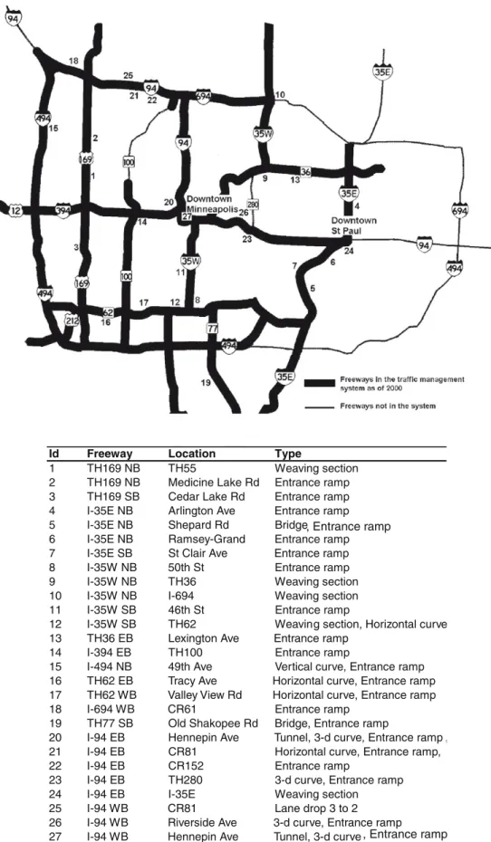
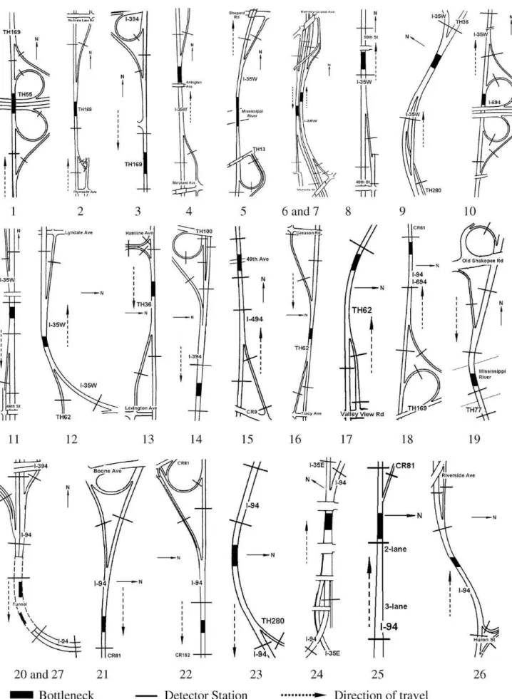
The above data filtering process excluded a surprisingly high number of bottlenecks from the analysis primarily due to detection errors. Out of several-hundred candidate sites, only 27 active bottlenecks identified by a methodology described later in Section4survived the above selection criteria. All of them are recurrent bottlenecks where the number of break-down occurrences during the metering-off period ranges from 8 to 74. The location and geometric characteristics of these studied bottlenecks are summarized in Figs. 1 and 2respectively. The sample has a good mix of various types of bottle-necks and some bottlebottle-necks have multiple characteristics that may cause traffic breakdown. A bottleneck is considered as a weaving section if it is a short joint section (<1 km) of two major freeways (bottlenecks 9, 12, and 24) or caused by weaving from both an on-ramp and an off-ramp (bottlenecks 1 and 10). Some bottlenecks are located near bridges with narrow shoulders or inside tunnels (bottlenecks 5, 19, 20, and 27). Some bottlenecks are located in freeway sections with visually identifiable horizontal curves (bottlenecks 12, 16, 17, and 21), or uphill grade along the direction of travel (bot-tleneck 15), or both (bot(bot-tlenecks 20, 23, 26, and 27). One bot(bot-tleneck is caused by lane drop from three to two (bot(bot-tleneck 25). If there is an on-ramp located no further than 1.6 km (one mile) upstream, a bottleneck is at least partially due to weaving from the on-ramp (bottlenecks 2–8, 11, 13–23, and 25–27), even though the average hourly peak period volume at several upstream on-ramps is not very high (<250 veh/h at bottlenecks 5 and 16). These categorization criteria tend to list all possible causes of traffic breakdown at each studied bottleneck, some of which might not be significant. However, there is no way to test the performance of those bottlenecks without one or more of the listed characteristics and to elim-inate the insignificant factors.

The locations of data detection stations with respect to the bottlenecks are also shown inFig. 2. Loop detectors are in-stalled at about 0.8-km (half-mile) intervals on Twin Cities freeways, and additional detection stations are inin-stalled in merg-ing and divergmerg-ing areas to ensure direct detection of traffic data in every freeway segment with uniform flow characteristics.

This allows us to gather flow and occupancy data no further than 0.4-km (a quarter mile) upstream and downstream of stud-ied bottlenecks.

Id Freeway Location Type

1 TH169 NB TH55 Weaving section

2 TH169 NB Medicine Lake Rd Entrance ramp

3 TH169 SB Cedar Lake Rd Entrance ramp

4 I-35E NB Arlington Ave Entrance ramp

5 I-35E NB Shepard Rd Bridge

6 I-35E NB Ramsey-Grand Entrance ramp

7 I-35E SB St Clair Ave Entrance ramp

8 I-35W NB 50th St Entrance ramp

9 I-35W NB TH36 Weaving section

10 I-35W NB I-694 Weaving section

11 I-35W SB 46th St Entrance ramp

12 I-35W SB TH62 Weaving section, Horizontal curve

13 TH36 EB Lexington Ave Entrance ramp

14 I-394 EB TH100 Entrance ramp

15 I-494 NB 49th Ave Vertical curve, Entrance ramp

16 TH62 EB Tracy Ave Horizontal curve, Entrance ramp

17 TH62 WB Valley View Rd Horizontal curve, Entrance ramp

18 I-694 WB CR61 Entrance ramp

19 TH77 SB Old Shakopee Rd Bridge, Entrance ramp

20 I-94 EB Hennepin Ave Tunnel, 3-d curve, Entrance ramp ,

21 I-94 EB CR81 Horizontal curve, Entrance ramp,

22 I-94 EB CR152 Entrance ramp

23 I-94 EB TH280 3-d curve, Entrance ramp

24 I-94 EB I-35E Weaving section

25 I-94 WB CR81 Lane drop 3 to 2

26 I-94 WB Riverside Ave 3-d curve, Entrance ramp

27 I-94 WB Hennepin Ave Tunnel, 3-d curve

, Entrance ramp

, Entrance ramp

3. Development of hypotheses

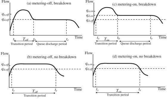
Breakdown refers to the transition of traffic from the uncongested state where small disturbances do not affect upstream traffic to the congested state at bottlenecks. After breakdown, a queue forms upstream of the bottleneck while the flow downstream remains uncongested. This state of a bottleneck is said to be active (Daganzo, 1997). On a time-series plot, breakdown is often associated with a sharp speed drop and sometimes a flow drop during a period of high demand. Two typical profiles of flow collected just downstream of a bottleneck without metering are plotted inFig. 3a (with breakdown) and inFig. 3b (without breakdown). InFig. 3a, the demand at the bottleneck increases at the beginning of the peak period. At timets, the flow equals the long-run average queue discharge flow of the bottleneck,qd,off. The subscript denotes metering

status (off or on). Then after a period of high flows (Toff), at timetba breakdown activates the bottleneck. We refer toToffas

the pre-queue transition period in the remainder of the paper. The average flow rate duringToffisqa,off. Aftertbthe bottleneck

operates at queue discharge flow rates (QDF) until it recovers atteor is deactivated by downstream congestion (this later

deactivation scenario is not shown inFig. 3). Afterte, the location may or may not experience another breakdown.Fig. 3b

shows another possible flow pattern at a bottleneck without metering. Again, as the demand increases,tswill be observed.

But the location does not experience a breakdown in this case possibly due to short duration of high demand or simply by chance. The duration ofToffandqa,offcan be similarly identified in this case, but not the QDFs. It should be noted that the

pre-queue transition flow,qa, computed under our definition is lower than that in previous papers (e.g.Cassidy and Bertini, 1999;

Hall and Agyemang-Duah, 1991; Banks, 1991a,b), because our approach takes into account both the rising and falling flows during the pre-queue transition period, not just the highest flow rate. Therefore, the readers should be aware that our meth-od underestimates the flow drop following bottleneck breakdowns compared to previous findings.

If ramp meters control the freeway where the bottleneck is located, one can also find the two typical flow profiles, one with and the other without breakdown (Fig. 3c and d). Likewise, the average QDF (qd,on), the duration of the pre-queue

tran-sition period (Ton), and the average flow rate during the transition period (qa,on) can be obtained. In those schematic graphs,

one may notice a long pre-queue transition periodT, constant QDF,qasignificantly higher thanqd, andqd,onsignificantly

higher thanqd,off. All these are for the sake of illustration and their real characteristics and relationships are subject to

sub-sequent statistical tests.

3.1. Hypothesis 1: Tonand Toffare not negligible

If this hypothesis is rejected by data, it implies whenever the demand at a bottleneck exceeds itsqd, breakdown occurs

and the bottleneck is activated. Therefore, the rejection of the hypothesis will also reject the two-capacity hypothesis that the flow at an active bottleneck drops after the queue formation upstream since the pre-queue flows have almost never been higher thanqdfor a meaningful amount of time. Previous studies (Hall and Agyemang-Duah, 1991; Persaud et al., 1998;

Cas-sidy and Bertini, 1999) show the duration of the transition period without ramp metering ranges from 3 to 32 min, though different definitions of the transition periodTare used. Also worth noting in these studies is that only transition periods fol-lowed by breakdowns are considered (Fig. 3a) while transition periods not followed by breakdowns (Fig. 3b) are ignored, which may underestimateT.

ts te qa,on qd,off Ton Time Flow (d) metering-on, no breakdown ts te qa,off qd,off Toff Time Flow (b) metering-off, no breakdown ts tb te qa,off qd,off Toff Time

Flow _{(a) metering-off, breakdown}

Transition period Queue discharge period

ts tb te qa,on qd,on qd,off Ton Time Flow (c) metering-on, breakdown

Transition period Queue discharge period

Transition period Transition period

Note: qa is the average flow rate during T.

3.2. Hypothesis 2: qa,off> qd,offand qa,on> qd,on

This hypothesis asserts that the average flow rate during the pre-queue transition period is significantly higher than the average queue discharge flow. Past studies have shown mixed results on this test, a summary of which is available inCassidy and Bertini (1999).

3.3. Hypothesis 3: Ton> Toff

This hypothesis states that ramp metering can prolong the pre-queue transition period, and delay or even eliminate breakdowns. It has been conjectured in several previous studies (e.g.Banks, 1991a,b), and often cited as a rationale for ramp metering. It has not been statistically tested against empirical data with and without an operational ramp control strategy. 3.4. Hypothesis 4: qa,on> qa,off

This hypothesis states that the average flow rate during the pre-queue transition period is higher with metering than without. A short reflection would suggest thatqa,onis most likely to be equal toqa,off, because when the freeway operates

at the free-flowing condition duringToffandTon, the average flow rates should only depend on demand patterns. The

hypoth-esis, if supported by the data, implies the breakdown probability at the same demand level depends on ramp control status (lower with metering).

3.5. Hypothesis 5: qd,on> qd,off

Several previous studies, using data either with or without metering, suggest that queue discharge flows at an active bot-tleneck are relatively constant over time (e.g.Cassidy and Bertini, 1999). If a breakdown occurs with metering,qd,onmay be

improved resulting from smoothed merging maneuvers and thus higher thanqd,off.

3.6. Hypothesis 6: ramp metering can increase the capacity of freeway bottlenecks

If hypotheses 3–5 are not rejected, hypothesis 6 is corroborated under any existing definition of capacity. It will be re-jected if all the above three are rere-jected. Otherwise, further tests are required. A specific definition of capacity is not given in this paper. Of course, a standard definition of capacity, as recommended by the Highway Capacity Manual may be adopted here, based on which hypothesis 6 can be tested against empirical data even without the previous five tests. However, we feel that this would unnecessarily reduce the value of the results. The impact of ramp metering on properties of pre-queue transition flows, duration of pre-queue transition periods, and queue discharge flows is essential for us to understand how ramp metering affects traffic conditions at freeway bottlenecks.

A t-test on the paired differences of two metering scenarios (one pair for each bottleneck) is performed to evaluate hypotheses 2–5. Hypothesis 1 will only be evaluated empirically since a statistical test onT> 0 will never be rejected and cannot provide any additional information. The only two assumptions of the paired-differencet-test are that the sample dif-ferences are randomly selected and the distribution of the population of paired difdif-ferences is normal. The first assumption should be satisfied because the 27 bottlenecks used in the study can be viewed as a random sample of all bottlenecks in the Twin Cities. The normality assumption for each hypothesis test is double-checked using the Shapiro–Wilk normality test (Shapiro and Wilk, 1965) and the normal probability plot. The test results show that all five normality assumptions (one for eacht-test) cannot be rejected (p-values range from 0.16 to 0.94).

4. Methodology

An active bottleneck is characterized by a queue upstream and uncongested flow conditions downstream. The foremost task of this section is to develop a reliable and effective method that can identify active bottlenecks by checking traffic con-ditions upstream and downstream of every freeway segment with valid data in the Twin Cities metro area during the two seven-week study periods. Section4.1summarizes several existing data diagnostic tools. The following Section4.2explains why an improved occupancy-based method is selected. Section4.3describes the occupancy-based method with two thresh-olds in detail, followed by a discussion on the calibration of the two occupancy threshthresh-olds (Section4.4). Section4.5compares the proposed method with an established diagnostic tool – transformed cumulative count curves (Cassidy and Windover, 1995).

4.1. Summary of existing methods for identifying active bottlenecks

Daganzo (1997)summarizes three methods for the identification of active freeway bottlenecks. If speed measurements are available, an increase in average point speed along the traffic flow direction indicates a possible bottleneck (speed meth-od). Similarly a decrease in occupancy or density along the direction of travel is also a practical indicator of active bottlenecks

(occupancy method). The third method is due toCassidy and Windover (1995)who check that waves on both sides of the bottleneck propagate away from it using transformed cumulative flow and occupancy curves (wave method). Other traffic characteristics have also been used in past studies to identify freeway breakdown, e.g. occupancy-volume ratio (Hall and Agyemang-Duah, 1991) and pure visual inspection of time-series plots (Persaud et al., 1998).

For both speed and occupancy methods,Daganzo (1997)warns that without information about the optimal speed or occupancy thresholds, a drop of those measures may also be detected due to a fast- or slow-moving platoons within a long queue. If not applied appropriately, these two methods could misdiagnose segments within long freeway queues as active bottlenecks, because each interchange engulfed in such a queue may exhibit a higher on-ramp flow than off-ramp flow ( Cas-sidy and Mauch, 2001; Windover and CasCas-sidy, 2001). The advantage of speed and occupancy methods is that the whole checking process can be automated and the algorithm does not involve further subjective judgment after the threshold val-ues are determined. The wave method keeps track of vehicle accumulation and is the most reliable of all existing data diag-nostic tools. In addition, the wave method is able to reveal some traffic features that cannot be displayed in other diagdiag-nostic methods. However, it requires for each breakdown occurrence visual identification of the start and end time of the pre-queue transition and queue discharge periods. The number of freeway sections under consideration in this study is on the order of several hundred, which is required to systematically identify active bottlenecks in a metropolitan area. For a study period of 14 weeks, there are more than a thousand breakdown occurrences that need to be analyzed. Therefore, the superior reliabil-ity of the wave method and the efficiency of the speed or occupancy method are both attractive. There are several choices: (1) Use the wave method, but examine only several bottlenecks instead of 27 and significantly shorten the study period to a few days instead of 14 weeks; (2) develop an expert system that first induces the visual inspection rules human researchers use, and then apply the rules to automatically execute the wave method; (3) improve the reliability of the speed or occu-pancy method while keeping their efficiency.

4.2. Selection of the data diagnostic tool

The impacts of ramp metering on different types of bottlenecks could be quite different. It is thus crucial for this study to include various types of bottlenecks with different geometry, traffic conditions and number of lanes. A previous study ( Lev-inson and Sheikh, 2002) concludes that although after the meters were shut-off in the Twin Cities freeway traffic clearly but slowly moves to a new equilibrium. Even at the end of the shut-off experiment, traffic fluctuation compared to historical data was still slightly higher. From this point of view, a longer study period would be desirable. Option 1 is eliminated for those reasons. The idea in option 2 is interesting and probably deserves a separate research project in its own right. Preliminary analysis of such an expert system suggests that data noise issues may pose a hurdle. Therefore, the final decision is to im-prove the reliability of the occupancy method and validate the imim-proved method by comparing it against the wave method for at least one bottleneck occurrence at each studied bottleneck.

The single loop detectors installed on Twin Cities freeways only provide flow and occupancy readings. To obtain speed estimates, the average vehicle length, which is a dynamic function of traffic composition, is needed. Such a step may introduce biases. Therefore, the occupancy method is selected over the speed method, though both methods should be about equally reliable. We understand that the validity of the traditional occupancy method based on a single thresh-old is questionable when they are used to detect active bottlenecks. A major improvement we propose is the adoption of two occupancy thresholds, thus creating a buffer zone to deal with the spatial (across bottlenecks due to sensitivity set-tings) and temporal variations (at the same bottleneck due to changing traffic composition) of the optimal occupancy threshold values.

4.3. A method for identifying active bottlenecks based on two occupancy thresholds

This section illustrates how the proposed occupancy-based method identifies active bottlenecks, and derives the average queue discharge flow (qd), duration of pre-queue transition periods (T), and average pre-queue transition flow (qa) for testing

hypotheses developed in Section3.

The general guideline in the development of this occupancy-based bottleneck identification algorithm is a conservative one – minimize the possibility that an inactive bottleneck is diagnosed as an active bottleneck. A freeway mainline detection station consists of several loop detectors with each corresponding to one lane. If the minimum occupancy of all lanes is above 25, which approximately corresponds to the density of 39 veh/lane/km with 5% trucks, the detection station is considered as congestedwithin a queue. If the maximum occupancy of all lanes is below 20 (approximately 31 veh/lane/km; Section4.4

explains why 25 and 20 are chosen as the thresholds), the detection station is considered asuncongested. Time intervals belonging to neither of the above two states areintermediateperiods. During the intermediate periods which are usually very short, breakdowns occur, and queues build up from one lane to all lanes, or from the bottleneck to the closest upstream sta-tion. Data analysis suggests that the duration of an intermediate period is almost never longer than 10 min. Therefore, all intermediate periods are simply excluded from the following computation of traffic parameters. This will slightly reduce the length of computed queue discharge periods and possibly pre-queue transition periods, but should not bias the hypoth-esis testing results in any significant way (see period 3 inFig. 4for an example; note only the time-series plot on the top of

Each freeway station in each 32 time interval must be under one of the following three conditions according to the occu-pancy readings across all lanes: congested, uncongested, or intermediate. Then each pair of adjacent freeway mainline sta-tions can be examined.

If the upstream station is congested while the downstream one is uncongested for more than five consecutive minutes, the freeway mainline section between the two stations is considered as an active bottleneck. The only exception is that the queue at the upstream station may be caused by insufficient off-ramp capacity if there is an off-ramp between the two

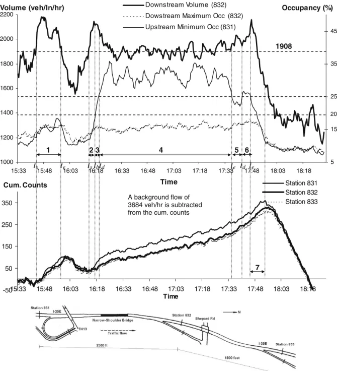
sta-1908 veh/ln/hr: long-run average queue discharge flow rate calculated from the 7-week study period; 1: The first observed pre-queue transition period (15 minutes, not followed by a breakdown); 2: The second pre-queue transition period (4 minutes, followed by a breakdown);

3: Intermediate period excluded from the analysis (3 minutes); 4: The first queue discharge period (1 hour 17 minutes);

5: A period lost due to conservative occupancy thresholds (5 minutes); 6: Another queue discharge period (5 minutes);

7: The end of the dissipating queue is between the bottleneck and station 831 during this period.

1000 1200 1400 1600 1800 2000 2200 15:33 15:48 16:03 16:18 16:33 16:48 17:03 17:18 17:33 17:48 18:03 18:18 Time Volume (veh/ln/hr) 5 15 25 35 45 Occupancy (%) Downstream Volume

Dowstream Maximum Occ Upstream Minimum Occ

1 2 3 4 5 6 1908 20

t

t

t

t

t

t

t

t

Cum. Counts Station 831

Station 832 Station 833 A background flow of

3684 veh/hr is subtracted from the cum. counts

7

tions (a diverge bottleneck). Therefore, traffic conditions at the off-ramp must also be considered. If the off-ramp station is congested, the freeway mainline section is not an active bottleneck because what is critical in this case is the capacity of the off-ramp, not the mainline section. Diverge bottlenecks are excluded from the analysis because it is unlikely that meters would have any impacts on the capacity of off-ramps (which actually depends on traffic and control on local streets). It should be noted that depending on the placement of the off-ramp detectors, a diverge bottleneck may be active even when the off-ramp detection station is not congested. This is caused by mainline exiting flow rates exceeding off-ramp capacity. Therefore, caution should be taken if the above method for identifying active freeway bottlenecks is applied to freeway loca-tions with off-ramps carrying high mainline exiting flows.

Once an active freeway bottleneck is identified, QDFs will be collected immediately downstream of the bottleneck until it is deactivated (see period 4 inFig. 4). If both the upstream and the downstream stations return to the uncongested state for more than 5 min, the beginning of that 5-min period is considered as the end of the preceding queue discharge period. There may be multiple queue discharge periods during a peak period. The average QDF of each afternoon peak period with and without ramp metering can be calculated (qd,offandqd,on). When flows in queue discharge periods across all studies days

are averaged, the long-run average QDF at each bottleneck is obtained. It should be mentioned that some studied freeway sections never experienced breakdown when meters were on in 1999. The variableqd,onis hence not available at these

loca-tions (14 out of 27 bottlenecks). The total number of queue discharging periods with and without ramp metering respec-tively are also recorded because they disclose whether ramp metering reduces breakdown occurrences.

If both the upstream and the downstream stations of a bottleneck are uncongested and the flow measured at the down-stream station is higher than the long-run average QDF during a 32 interval, that interval is a part of the pre-queue transition periodTbecause the demand during that interval is high enough to potentially cause a breakdown (see period 2 inFig. 4). There may be multiple pre-queue transition periods during a peak period, and a transition period may not be followed by a queue discharge period (see an example of non-breakdown transition period inFig. 4– period 1). Since previous studies do not consider non-breakdown transition periods and only report the average duration of breakdown transition periods, these two types of queue transition periods are distinguished in the analysis to facilitate comparison to earlier work. If a pre-queue transition period ends and a subsequent pre-queue discharge period starts within 10 min (a 10-min threshold is adopted to account for the short intermediate period – such as period 3 inFig. 4), this pre-queue transition period is associated with the breakdown. Otherwise, it is considered as a non-breakdown transition period. The total length of all transition periods (T) throughout an afternoon peak period is computed and used in the hypothesis testing. The flow rates in the transition periods are collected by the same set of detectors that collect QDFs (i.e. the detection station immediately downstream of the bot-tleneck). The average flow during the transition period isqa. The computation ofTandqausesqd,offfor both metering-on and

-off periods, so the results with and without metering are comparable.

If the downstream station of a freeway section is congested, the traffic condition at the current section is determined by active bottlenecks further downstream. These observations are excluded from the analysis of the current freeway section. An example of such situations is included in the following section.

One conceivable drawback of the traditional occupancy method is that when a freeway section is within a long queue, a decrease in occupancy along the direction of travel may still be observed in that section because traffic entering from the on-ramps consumes mainline capacity (Cassidy and Mauch, 2001). Two data selection criteria are adopted in the improved method to address this issue – only bottlenecks with more than eight breakdown observations are included in the analysis, and only queue discharge periods longer than 5 min are considered as real queue discharge periods. The occupancies mea-sured at a short distance upstream of a bottleneck can be relatively low during some time intervals. But the duration of the low occupancy readings (<20% used in this analysis) within a queue is rarely longer than 5 min across all lanes. With these two additional requirements in the occupancy method, the likelihood that a segment within a queue is misdiagnosed as ac-tive bottlenecks should be very small, if not zero.

The occupancy method uses the maximum occupancy of all lanes at the downstream station (with respect to the active bottleneck) and the minimum occupancy of all lanes at the upstream station to determine if a section is congested or not. Although this technique effectively reduces the chance of misdiagnoses, it could make the method more restrictive (requir-ing worse conditions) as the number of lanes increases because typically one or more lanes frequently exhibits a lower occu-pancy than the others during congestion. As a result of this fact, it is possible that at a mildly congested bottleneck breakdown is not detected by the occupancy method until much later and artificially extending the pre-queue discharge per-iodT. After categorizing results by number of lanes at the bottlenecks (see Note a inTable 1in Section5), there is no evidence that this type of misdiagnosis occurred in our analysis – the percentage increase of the pre-queue transition period is not higher at bottlenecks with more lanes. But the described situation might occur had an upper-bound occupancy threshold higher than the 25% used in this analysis been selected.

4.4. Calibration of the two occupancy threshold values

We sampled more than thirty breakdowns at several well-known bottlenecks on Trunk Highway 169 and I-94 in order to decide which threshold values to use in the occupancy method. Time-series occupancy and flow data, as well as cumulative count curves, were plotted for all breakdown observations in the sample in a fashion similar toFig. 4, where the effectiveness of alternative occupancy thresholds can be tested. Visual inspection was used to identify the ‘‘optimal” threshold values on the plots. The starting point of the search for the threshold values in the experiment is 18%, which is used by the Minnesota

Department of Transportation to separate congested and uncongested flow. We found that 18% is a bit low; 20% and 25% were finally selected because this combination identifies pre-queue transition periods and queue discharge periods better than other combinations based on visual inspection (a combination is better if the high threshold value crosses the upstream minimum occupancy line and the low threshold value crosses downstream maximum occupancy line less often during an observable queue discharge period). More evidence of the superiority of this combination is provided in the following two examples. Thanks to the 5% buffer zone (20–25%), the method performs well on different bottlenecks even with the same two threshold values. Adopting spatially dependent threshold values at different bottlenecks only improves the data diagnosis process marginally (shorter intermediate periods which are already very short); and still does not address tempo-ral variations. The two threshold values were later validated using at least one breakdown observation from all 27 studied bottlenecks.

4.5. Comparison against the wave method

The improved occupancy method is compared with the wave method (Cassidy and Windover, 1995) at the studied bot-tlenecks and two representative examples are shown below to demonstrate its reliability. The first example is still at bottle-neck 5 on November 21, 2000 (meters are off) as illustrated inFig. 4.

The bottleneck is located on I-35E in Saint Paul between stations 832 and 831, and is caused by a bridge on Mississippi River with a narrow shoulder lane and the entrance ramp from TH13. The improved occupancy method (upper graph) cor-rectly identifies the two pre-queue transition periods (periods 1 and 2), which is verified by the cumulative count curve (lower graph). It should be noted that the cumulative count curve also shows the existence of two transient queues upstream of the bottleneck but downstream of station 831 during period 1. This feature cannot be detected on the time-series plot. But clearly, the bottleneck was not activated in this period. The real breakdown occurred at about 16:18. It is also now clear that during period 3, an intermediate period excluded from the analysis, the queue propagated upstream and reached station 831 at the beginning of period 4. The occupancy method collects queue discharge flow rates in period 4, which was indeed a part of the queue discharge period at bottleneck 5 on that day because the queue between station 831 and station 832 is evident

Table 1

Some traffic characteristics at all studied active bottlenecks with ramp metering on and off. Id # Lanesa _{# Days Breakdown}

per day

qd(veh/h) T(hh:mm/day)bTb(mm/breakdown period)Tnb(mm/

non-breakdown period)

qa(veh/h)

Off On Off On Off On D(%) OffTb OffTnb OnTb OnTnb OffT OnT D(%) Off On D(%)

1 2 24 29 3.1 1.6 4152 4349 5 9 7 37 45 0:13 1:21 523 4237 4419 4 2 2 26 29 2.1 0.4 3991 3997 0 18 13 86 77 1:08 2:37 131 4223 4328 2 3 2 27 24 0.3 0 4107 NA NA 10 8 NA 19 0:27 0:35 30 4256 4298 1 4 3 28 29 0.3 0.2 5885 6115 4 27 30 8 92 1:54 2:33 34 6396 6490 1 5 2 27 29 0.8 0 3816 NA NA 30 10 NA 18 1:08 1:03 !7 4052 4078 1 6 2 26 29 1.2 0 3900 NA NA 5 6 NA 16 0:22 1:11 223 4016 4042 1 7 2 27 29 0.4 0 4019 NA NA 4 11 NA 24 0:44 1:07 52 4179 4212 1 8 3 28 28 0.9 0.5 5694 5679 0 18 22 32 56 2:59 3:18 11 6156 6165 0 9 4 27 28 0.4 0 8336 NA NA 14 8 NA 73 0:36 2:03 242 8837 9291 5 10 3 27 29 2.1 0 6728 NA NA 9 10 NA 82 0:04 1:27 2075 6885 7329 6 11 3 26 28 0.7 0 6650 NA NA 8 8 NA 18 1:13 1:58 62 6851 6892 1 12 3 27 28 0.7 0.8 5243 5079 !3 13 13 14 20 3:05 1:34 !49 5490 5389 !2 13 2 27 28 0.5 0 4206 NA NA 15 13 NA 16 0:40 0:49 23 4430 4304 !3 14 3 27 29 2.6 1.8 5196 5393 4 14 10 38 30 1:04 1:36 50 5450 5396 !1 15 2 26 29 1.3 0 4165 NA NA 14 8 NA 22 0:14 1:24 500 4264 4313 1 16 2 24 29 1.2 0 4004 NA NA 15 12 NA 23 0:38 1:19 108 4258 4240 0 17 2 26 29 0.5 0 3876 NA NA 5 6 NA 16 1:08 1:14 9 4028 3997 !1 18 2 23 28 2.2 1.0 3867 3882 0 6 11 30 49 0:53 1:54 115 4054 4161 3 19 3 27 29 0.2 0 6122 NA NA 3 11 NA 45 0:49 1:12 47 6418 6580 3 20 3 28 9 0.3 0 5415 NA NA 50 18 NA 61 1:43 2:28 44 5664 5771 2 21 2 26 28 1.7 0.5 3670 3599 !2 10 9 46 29 1:05 2:14 106 3865 3846 0 22 2 28 28 0.8 0.2 3588 3793 6 32 21 0 103 2:36 3:41 42 3914 4008 2 23 3 27 29 2.3 1.4 6063 6250 3 14 9 79 61 0:49 2:19 184 6348 6559 3 24 4 24 29 1.8 0.7 7335 8023 9 38 26 3 133 0:58 2:45 184 8136 8773 8 25 2 28 28 1.3 1.8 3771 3911 4 31 12 107 58 1:33 2:52 85 4021 4149 3 26 3 28 29 0.3 0.5 5205 5688 9 NAc _{12 0 65 1:56 4:08 114 5655 5822 3} 27 3 28 9 1.2 0 5476 NA NA 55 26 NA 88 1:03 3:08 198 5847 5979 2 Ave. 27 27 1.2 0.4 4981 5058 3 18 13 37 50 1:08 1:59 73 5257 5360 2

a _{The percentage increase ofTis 82% for the fourteen 2-lane bottlenecks, 54% for the eleven 3-lane bottlenecks, and 206% for the two 4-lane bottlenecks.} b _{Tis the total duration of all pre-queue transition periods per day which is used for hypothesis testing.T}

b(Tnb) is the average duration of (non-)

breakdown transition periods.TbandTnbare calculated for comparison with previous studies that do not include non-breakdown transition periods. See

Section4for more detailed definition of those variables.

and no queued vehicle existed between station 832 and station 833. Period 5 was also a part of the queue discharge period, but is not detected by the occupancy method due to low occupancy at the upstream station 831. We found that the flow from the on-ramp at TH13 was relatively low just before and during period 5 so that the mainline traffic at station 831 could move faster and caused a temporary fast-moving low-occupancy platoon within the long queue upstream of the bottleneck. The occupancy method continued to collect queue discharge flows during period 6 while missing period 7. The end of the queue was between station 831 and the bottleneck during period 7 before it finally dissipated at about 17:55. Discarding periods 5

1 2 3 4

6 5

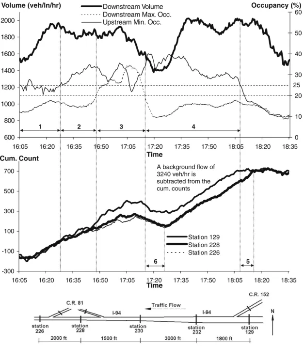
1. It is evident in this period that the occupancy method with two thresholds is better than with only one threshold; 2. Bottleneck 25 (between stations 228 and 230) is activated and display queue discharge flow;

3. Bottleneck 25 is deactivated by a more restrictive bottleneck downstream as the high occupancy values at station 228 and queuing between station 228 and station 226 both suggest;

4. Bottleneck 25 again become active after the bottleneck further downstream is relieved;

5. Bottleneck 25 is deactivated and queue dissipates between the bottleneck and station 129 during this period due to reduction of travel demand.

6. A period when the flow at bottleneck 25 recovers fro m the lower queue discharger flow of the downstream bottleneck to its own queue discharge flow;

A background flow of 3240 veh/hr is subtracted from the cum. counts 25 600 800 1000 1200 1400 1600 1800 2000 16:05 16:20 16:35 16:50 17:05 17:20 17:35 17:50 18:05 18:20 18:35 Time 0 10 20 30 40 50 60 Downstream Volume Downstream Max. Occ. Upstream Min. Occ.

Occupancy (%) Volume (veh/ln/hr) -300 -100 100 300 500 700 16:05 16:20 16:35 16:50 17:05 17:20 17:35 17:50 18:05 18:20 18:35 Time Cum. Count Station 129 Station 228 Station 226

and 7 in this particular example could cause a slight underestimation of the average queue discharge flow. It is likely that a slight overestimation might occur on some other days. But over the long run, there should not be significant systematic biases. Lastly, the low occupancy threshold, 20%, performs very well in this example. An even lower threshold, such as 18%, could misdiagnose station 832 as congested during periods 4 and 6.

Let us now move to an example that is somewhat more complicated than the previous one. Bottleneck 25 inFig. 5is on I-94 WB between stations 228 and 230 due to a lane drop from three to two lanes just upstream of station 230. By examining the cumulative curves (lower graph) at stations 226, 228, and 129 (curves for stations 230 and 232 are not shown to improve the clarity of the graph without loss of important information), we found that on November 20, 2000 (meters were off), this bottleneck was activated at 16:29 (period 2: queue started to build up between stations 228 and 129, but not downstream of station 228), deactivated by a bottleneck further downstream at 16:45 (period 3: queue started to build up between station 226 and 228), again activated after the bottleneck further downstream was relieved around 17:20 (periods 4 and 5), and fi-nally deactivated as demand dropped at 18:15. The reliability of the occupancy method (upper graph) is again almost equally good. It accurately identifies periods 2 and 4 when the bottleneck was active (high occupancy upstream but low occupancy downstream), and period 3 when the bottleneck was deactivated (high occupancy downstream). Using the maximum down-stream occupancy across all lanes seems to be good practice to ensure that period 3 would not be misdiagnosed as a queue discharge period for bottleneck 25. The only controversy arises with respect to period 6 when the flow at bottleneck 25 recovered from the lower queue discharge flow of the further downstream bottleneck to its own higher queue discharge flow. The occupancy method considers this period as a part of the queue discharge period for bottleneck 25. Looking at the cumulative count curve, one would agree that the impact of the bottleneck further downstream still existed during per-iod 6. At the same time, it is also evident that the queue downstream of station 228 had already dissipated before perper-iod 6. The behavior of that recovery wave is certainly interesting but beyond the scope of this paper. Another point worth noting in this case is the selection of the high-occupancy-threshold (25% used in the analysis). This bottleneck location requires the highest high-occupancy-threshold, probably due to an extreme detector sensitivity setting. Let us take period 1 as an exam-ple. There was a short occupancy spike in period 1. It would not be considered as a queue discharge period by the occupancy method because it is shorter than 5 min, which avoids a misdiagnosis. Any high-occupancy-threshold lower than 25% would result in a misdiagnosis. Also conceivable is that if an occupancy method with a single threshold between 18% and 25% was used, it would misdiagnose period 1 as a queue discharge period. The value of the 5% buffer zone in the improved method with two occupancy threshold is evident in this example.

By using two thresholds, adding constraints on minimum shortest queue discharge periods, and analyzing only recurrent bottlenecks, the improved occupancy method described above as a tool for systematically identifying and analyzing active bottlenecks, satisfactorily marries efficiency and reliability for the purpose of this study.

5. Results

The actual number of days studied at the 27 bottlenecks varies due to weather, accidents, and detector failures. On aver-age, 27 days were examined with and without metering respectively. This section interprets test results of the six hypoth-eses, as well as some other interesting findings.

Some traffic characteristics related to hypothesis testing are summarized inTable 1. Detailedt-test results are presented inTable 2. Hypothesis 1 is supported. The average duration of transition periods per peak period (T) is about 68 min without metering. It is also evident from the data that multiple breakdowns could occur during a peak period, and flow at a bottle-neck could be higher than the long-run queue discharge flow for a long period of time without causing a subsequent break-down (non-breakbreak-down transition periods). After separating transition periods followed by breakbreak-downs from those not followed by breakdowns, we found that the average duration of breakdown transition periods without metering (off Tb) is

about 18 min (standard deviation 13 min). This falls within the range found in past studies (3–32 min per breakdown) which did not consider non-breakdown transition periods.

Hypothesis 2 (qa,off>qd,off,and qa,on>qd,on) is confirmed. The definition of the pre-queue transition period determines that

qawould be larger thanqd. What matters is really how muchqais larger thanqd. It is found from the data that on averageqa,off

is 5.5% higher thanqd,off, andqa,onis 5.8% higher thanqd,on. These percentage flow drops observed under both control

scenar-ios are statistically significant at level 0.01 (see the first two rows inTable 2). The flow drops at all studied bottlenecks after

Table 2

Hypothesis testing results.

Hypothesis One-tailed paired-differencet-test Hypothesis confirmed? % Change NullH0 AlternativeHa t p H0rejected?

qa,off>qd,off qa,off=qd,off qa,off>qd,off 9.14 0.00 Yes (df = 26) Yes +5.5

qa,on>qd,on qa,on=qd,on qa,on>qd,on 5.74 0.00 Yes (df = 12) Yes +5.8

Ton>Toff Ton=Toff Ton>Toff 5.73 0.00 Yes (df = 26) Yes +73.4

qa,on> qa,off qa,on=qa,off qa,on>qa,off 3.18 0.00 Yes (df = 26) Yes +2

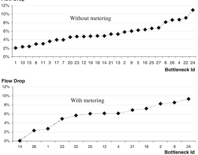
breakdown range from 2% to 11% with a standard deviation of 2.2% without metering, and 0.1% to 9% with a standard devi-ation of 2.6% with metering. We should emphasize that these are percentage flow drops following bottleneck breakdowns,

Without metering

With metering

Bottleneck Id

Flow Drop

Bottleneck Id

Flow Drop

Note: Only thirteen bottlenecks still experienced breakdown with ramp metering.

not capacity drops. Additional test results strongly suggest that the percentage flow drops at various bottlenecks are nor-mally distributed (Normality can not be rejected at level 0.91 according to the Shapiro–Wilk test; seeFig. 6). Previous studies have drawn conflicting conclusions on this issue. Some found high percentage flow drops and considered their findings as evidence of the two-capacity hypothesis (Banks, 1991a,b; Hall and Agyemang-Duah, 1991). Others observed very small flow differences and concluded that even if the two-capacity phenomenon ever exists, it does not provide a rationale for ramp metering (Newman, 1961; Newman et al., 1969; Persaud, 1986; Persaud and Hurdle, 1991). Our results suggest that insuf-ficient sampling from the underlying normal distribution may lead to inconsistent conclusions because no more than four bottlenecks were examined in the cited research. If this argument is true, it becomes important to understand what factors contribute to the normal variability. In that case, detailed analysis at individual bottlenecks is necessary. An alternative view is offered byCassidy and Bertini (1999), who attribute the inconsistency to the inadequate data analysis methods used in those studies.

Whether meters are able to prolong the pre-queue transition period is examined by hypothesis 3 (Ton>Toff). The average

duration of transition periods in an afternoon peak period increases by 73% from 68 min without metering to almost two hours with metering. The magnitude of such increase varies from location to location, but is statistically significant at level 0.01. The average number of breakdown occurrences has also been reduced from 1.2 without metering to 0.4 per bottleneck per afternoon peak period with metering. According to these results, the ramp control strategy is able to not only extend transition periods and delay bottleneck activations, but also eliminate a significant number of breakdowns. At two bottle-necks (5, a bridge, and 12 a weaving section where I-35E southbound and TH62 westbound join), the transition periods are actually shorter with metering, which may be explained by the decreased demand at these two locations in 2000.

Another surprising finding is that hypothesis 4 (qa,on>qa,off) is also confirmed. The average flow rate in the pre-queue

transition period is about two percent higher with metering than without metering, when averaged across all studied bot-tlenecks. The difference is statistically significant at level 0.01. This implies that at the same demand level, breakdown at a bottleneck is less likely to occur if ramp meters control the freeway.Persaud et al. (2001)propose a probabilistic ramp con-trol logic to maximize the expected benefits based on the observed breakdown probability distribution. If the breakdown probability function itself shifts as ramp meters are deployed, one should base metering rates on the distribution estimated from metering-on data. Future studies can estimate and compare the breakdown probability distributions with data col-lected under both control scenarios, and summarize the implications for the design of efficient and reliable ramp control strategies.

The assumption of constant QDFs at the same bottleneck regardless of metering status has been made in numerous the-oretical and practical ramp metering studies. Many believe that once a bottleneck is activated, ramp metering would no longer make a difference and emphasize solely its role of delaying breakdown onset. However, our results suggest that this assumption is not true. Across all studied bottlenecks, qd is more than three percent higher with metering than without

metering. The null hypothesis that the two are equal is rejected at level 0.01. At two locations,qd,onis as much as nine percent

higher thanqd,off(24: a weaving section; and 26: a busy entrance ramp with combined horizontal and vertical curves). A

pos-sible explanation is that when an activated bottleneck is not metered, a platoon of merging and/or diverging vehicles may cause intensive short-term lane-changing maneuvers on freeway mainline sections, which may lead to further speed drops and thusqddrops. Another explanation, suggested by an anonymous reviewer, is that QDF at weaving bottlenecks (and

bot-tlenecks with high merging on-ramp flow) is a function of weaving flow determined by freeway OD patterns. The weaving patterns likely changed after the meters were turned off because meters explicitly favor mainline traffic at the expense of ramp traffic. Future studies should examine the causes of lower qd without metering with higher quality data.Cassidy

Table 3

Impacts of traffic growth on bottleneck flow characteristics.

Id Study period (days) Breakdowns per day qd(veh/h) T(hh:mm/day) qa(veh/h)

1999 2000 1999 2000 1999 2000 D(%) 1999 2000 D(%) 1999 2000 D(%) 1 27 23 3.0 1.7 4343 4378 1 0:22 0:37 68 4404 4405 0 2 28 23 0.3 0.6 3958 3985 1 2:43 2:41 !1 4307 4330 1 4 28 25 0.1 1.5 5862 6002 2 2:39 2:03 !23 6461 6475 0 6 27 25 1.0 0.1 3950 3608 !9 0:36 0:52 44 4045 4073 1 7 28 24 0.2 0 4121 NA NA 0:46 1:00 30 4235 4293 1 9 28 24 0.1 0.2 9095 8626 !5 1:53 1:17 !32 9580 9525 !1 14 27 23 2.5 1.2 5309 5333 0 0:50 0:55 10 5446 5420 0 15 28 25 0.9 0.1 4103 4043 !1 1:08 1:34 38 4252 4276 1 16 25 24 0.2 0.1 3862 3712 !4 1:39 1:14 !25 4154 4081 !2 23 27 23 2.7 1.8 6235 6327 1 1:08 1:34 38 6522 6601 1 26 28 24 0.1 0.1 6012 6051 1 1:43 1:23 !19 6221 6204 0 Ave. 27 24 1.0 0.7 5273 5207 !1 1:24 1:22 !2 5421 5426 0

Note: ‘‘2000” refers to the week period immediately before the shut down experiment (August 28–October 13, 2000). ‘‘1999” refers to the seven-week period in 1999 (August 30–October 15, 1999) that corresponds to the ‘‘2000” period. The purpose of this analysis is to test whether the changes revealed inTable 1are simply due to annual traffic growth, and that hypothesis is rejected. Ramp metering was on during both periods reported in this table.

and Rudjanakanoknad (2002)collected arrival times of individual vehicles at a merging bottleneck and found slow-downs even after breakdowns.

Since hypotheses 3–5 are all confirmed by the data, hypothesis 6 is also supported. Ramp metering increases the capacity of freeway bottlenecks in three ways: metering postpones and sometimes eliminates bottleneck activation, it accommodates higher flows during the pre-queue transition period than without metering, and it increases queue discharge flow rates after breakdown. Various parameters defined in the Minnesota zonal ramp control strategy, such as bottleneck flow thresholds, and even the algorithm itself are not necessarily optimal. Therefore, this study may have underestimated the capability of ramp meters. In order to explore the full potential of ramp meters in improving bottleneck capacity, more elaborate exper-iments in which metering rates can be changed over time are required.

It should be noted that ramp meters increased bottleneck capacity in 1999, when the overall system demand is lower than the metering-off period in 2000 due to annual traffic growth. Thus, it is reasonable to suspect that the observed capacity improvements with metering are simply due to lower demand. To explicitly control for annual traffic growth, all the analyses were repeated for the seven weeks (August 28–October 13, 2000) preceding the metering-off period. This reveals if there are similar results comparing to the corresponding seven new weeks in 1999 (August 30–October 15, 1999). If hypotheses 3–5 are also supported by this new data set, traffic growth clearly plays a role in capacity increases. If they are all rejected, the observed capacity increase at bottlenecks should be mostly attributed to ramp meters. The analysis on the new data set can only be performed at 11 of all 27 study sites for two reasons. First, there were not enough breakdown observations at some locations during the two new seven-week periods because ramp meters were present in both periods. The other reason is related to detector failure. Many corrupt detectors were repaired or replaced immediately before the shut down experiment, which means some bottlenecks with valid traffic data during the metering-off period did not meet the same data require-ments during the new seven-week period in 2000. Results of this additional analysis are summarized inTable 3. Hypotheses 3–5 are all rejected, and no statistically significant differences exist betweenqd,T, orqaduring the two new seven-week

peri-ods. Therefore the hypothesis that the observed capacity increase is simply due to traffic growth (or decline) is rejected. An aggregated approach is followed and results from 27 bottlenecks are combined together in this research to study the relationships between ramp metering and bottleneck capacity. However, insights might be lost in the aggregation and there might be advantages to giving more individualized attention to bottlenecks. As seen inTable 1, capacity improvement at dif-ferent sites varies. InTable 4.1, results are reported for each class of bottlenecks in an attempt to attribute this variation to bottleneck types. Considering some bottlenecks belong to multiple categories, we also performed a regression analysis (see resultsTable 4.2). It seems that ramp metering can most effectively improve bottlenecks that involve weaving sections, en-trance ramps, vertical curves and lane drop, while making little difference at bottlenecks that are bridges/tunnels, or have horizontal curves. Future studies may analyze data at individual bottlenecks in greater detail to provide conclusive findings on why queue discharge flows are higher, transition flows higher, and transition periods longer with ramp metering.

Table 4.1

Results: capacity improvement by bottleneck types.

Bottleneck type % Change inqd % Change inT % Change inqa

Weaving 3.7 5.9 4.4 On-ramp 3.5 2.0 1.8 Bridge/tunnel NA 0.7 1.8 Horizontal curve 1.8 0.8 1.0 Vertical curve 6.2 2.1 2.3 Lane drop 3.7 0.8 3.2 Table 4.2

Regression results: capacity improvement as a function of bottleneck types. Bottleneck type Dependent variables

% Change inqdn= 13,R2= 0.7 % Change inT/100n= 27,R2= 0.40 % Change inqan= 27,R2= 0.71

Weaving 4.8* _6.7*** _5.3*** On-ramp 6.0 7.5* _7.5*** Bridge/tunnel Dropped !0.72 0.5** Horizontal curve !4.2 !0.57 !0.02 Vertical curve 8.1* _{1.94 1.7}* Lane drop 7.4 7.5 10.1*** Constant !3.7 !6.6 !6.9***

Notes: Numbers shown are regression coefficients; all bottleneck types are treated as (0, 1) dummy variables.

* _{Statistically significant at level 0.1.} ** _{Statistically significant at level 0.05.} *** _{Statistically significant at level 0.01.}

A large number of flow measurements are recorded at the studied bottlenecks, which enables us to examine the distri-butions of transition flows and discharge flows per interval, per breakdown, and per peak period. The characteristics of these distributions have important bearing on the definition of freeway capacity. A detailed analysis of this issue is, however, be-yond the scope of this paper; interested readers are referred toZhang and Levinson (2004b).

6. Conclusions

Traffic flow characteristics at 27 active freeway bottlenecks in the Twin Cities are studied for seven weeks without ramp metering and seven weeks with ramp metering. A series of hypotheses regarding the relationship between ramp metering and the capacity of active bottlenecks are developed and tested against empirical traffic data. The results demonstrate with strong evidence that ramp metering can increase bottleneck capacity. It achieves that by:

(1) Postponing and sometimes eliminating bottleneck activation – the average duration of the pre-queue transition period across all studied bottlenecks is 73% longer with ramp metering than without;

(2) accommodating higher flows during the pre-queue transition period than without metering – the average flow rate during the transition period is 2% higher with metering than without (with a 2% standard deviation); and

(3) increasing queue discharge flow rates after breakdown – the average queue discharge flow rate is 3% higher with metering than without (with a 3% standard deviation).

Therefore, ramp meters can reduce freeway delays through not only increased capacity at segments upstream of bot-tlenecks (type I capacity increase), but also increased capacity at botbot-tlenecks themselves (type II capacity increase). Pre-viously, ramp metering is considered to be effective only when freeway traffic is successfully restricted in uncongested states. The existence of type II capacity increase suggests there are benefits to meter entrance ramps even after breakdown has occurred. This study focuses on the impacts of ramp metering on freeway bottleneck capacity. The causes of such im-pacts should be more thoroughly examined by future studies, so that the findings can provide more guidance to the devel-opment of ramp control strategies. It should also be noted that both types of capacity increases on the freeway mainline are at the expense of degraded conditions at the on-ramps and possibly arterial network. Therefore, without more com-prehensive system-wide analysis, the findings of this paper, though in favor of ramp metering, do not necessarily justify its deployment.

Type I and type II capacity increases and metering rates are highly correlated. The premise of type I capacity increase is that the bottlenecks are not activated or the physical queues upstream of bottlenecks do not block exit ramps. The tradeoff here is that metering rates should not be too low such that demand is overly restricted, and should not be too high such that queues form. The traditional metering goal of keeping the flow at a bottleneck strictly below its capacity should provide an optimum solution to this tradeoff. However, this goal may not adequately exploit the correlation between the type II capac-ity increase and metering rates since an always free-flowing freeway, which dictates low control threshold values (optimal volume or density), is not the best solution. In that case, the ability of ramp meters to postpone bottleneck activation and to increase queue discharge flow rates is wasted. Somewhat more aggressive threshold values may improve the overall effec-tiveness of ramp metering. To maximize the type II capacity increase, a set of rules associating metering rates and real-time flow conditions (mainline, merging and diverging flows and occupancy, etc.) are required. Improved driver behavior models and careful examination of traffic features at bottlenecks with high-quality data are both promising research approaches. It should also be remembered that type I and type II capacity increases tend to compete with each other when a controlled freeway is uncongested. For that reason, multiple metering logics corresponding to different freeway traffic conditions (maybe before and after breakdown) should be considered. These propositions have a long way to go before shedding light on the practical design of control logic. A direct implication of the findings in this study is that when selecting the threshold flow values for bottlenecks, engineers should not simply rely on the long-run queue discharge rate collected during a meter-ing-off period. A markup of that value estimated locally with empirical study may improve the efficiency of the algorithm. This study arrives at most findings by combining data from many different bottlenecks. Although the aggregation pro-vides an opportunity to examine distributional effects of some important bottleneck properties, it represents a limitation of this work – additional attention should be paid to the traffic evolution at individual bottlenecks. Diagnostic tools, such as curves of cumulative traffic counts and occupancy (Cassidy and Windover, 1995), should be considered to address this limitation.

Finally, it should be noted that the results presented in this paper are all based on traffic data collected in the Twin Cities with the same ramp control strategy. Similar analysis in other metro areas may provide additional insight. Also after the shut down experiment in 2000, a new algorithm with less restriction on on-ramp inflows and more equity considerations has been deployed in the Twin Cities, which provides an opportunity to empirically test the potential causes of increased bot-tleneck capacity.

Acknowledgements