Space Launch System Aeroacoustic Wind Tunnel Test Results

Space Launch System Aeroacoustic Wind Tunnel Test Results

Thomas B. Steva,∗Victoria J. Pollard,†and Andrew J. Herron‡ NASA George C. Marshall Space Flight Center, Huntsville, Alabama, 35812

Characterization of accurate launch vehicle unsteady aerodynamics is critical for compo-nent and secondary structure vibroacoustic design. For the National Aeronautics and Space Administration’s’s (NASA) Space Launch System (SLS), aeroacoustic environments have been derived primarily through sub-scale wind tunnel testing. Both optical techniques and high frequency pressure measurements have been utilized across multiple testing facilities and nu-merous vehicle configurations to develop a range of preliminary and detailed environments. As the vehicle has matured and evolved, the data collected from each subsequent configura-tion has allowed for comparison studies which isolate the effects of certain outer mold line (OML) features on measured fluctuating pressure levels. This paper presents observations on some of those effects for features which include abort system protuberances, various fairings geometries, interstage flanges, and multibody interactions between a central core and fall away boosters. These features, and the flow conditions produced by them, are broadly applicable to many launch vehicle configurations.

Nomenclature

AAT = SLS Ascent Aeroacoustic Wind Tunnel Test ARC = NASA Ames Research Center

AUAT = SLS Ascent Unsteady Aerodynamics Wind Tunnel Test CFD = computational fluid dynamics

dB = decibels referenced to 20x10-6 Pa DSC = data system coordinator

ES = engine section

ESM = Encapsulated Service Module EUS = Exploration Upper Stage EV33 = MSFC Aerosciences Branch

f = frequency

FPL = fluctuating pressure level l = characteristic length

LaRC = NASA Langley Research Center LAS = Launch Abort System

LH2 = liquid hydrogen LOX = liquid oxygen

LVSA = Launch Vehicle Stage Adapter Lp,M S = model scale narrowband FPL MPCV = Multi-Purpose Crew Vehicle MSA = MPCV Stage Adapter

MSFC = NASA Marshall Space Flight Center OAFPL = overall FPL

OML = outer mold line Pr e f = reference pressure

pr ms = root-mean-square acoustic pressure PSD = power spectral density

q∞ = free stream dynamic pressure ∗

Aerospace Engineer, Aerosciences Branch, EV33

†

Aerospace Engineer, Aerosciences Branch, Jacobs ESSCA

‡

Aerospace Engineer, Aerosciences Branch, EV33

RBOS = retro-reflective background oriented schlieren SLS = Space Launch Sytem

SRB = solid rocket booster St = Strouhal number T = static temperature

TWT = MSFC Aerodynamics Research Center Trisonic Wind Tunnell U = flow velocity

UPWT = ARC Unitary Plan Wind Tunnels USA = Upper Stage Adapter

VSS = Vehicle Stabilization System α _{= angle of attack}

αT = total angle of attack,(α2+β2)1/2 β = sideslip angle

∆Cp,r ms = nondimensional FPL coefficient

Φsc = structural coordinate system clocking angle

Notice to Readers

The predicted performance and certain other features and characteristics of the Space Launch System vehicle are defined by the U.S. Government to be Sensitive But Unclassified (SBU). Therefore, values in plots and figures have been either removed or normalized to arbitrary values.

I. Introduction

C

haracterization of accurate flight vehicle unsteady aerodynamics is critical for component and secondary structurevibroacoustic design and qualification. Empirical methods exist to attempt prediction of external fluctuating pressure levels (FPLs) induced during vehicle ascent, however the uncertainty of such methods can result in either an under-conservative or over-under-conservative design. Neither of these outcomes is desirable. Scaling wind tunnel and flight data from similar launch vehicles or protuberances generally yields better results, but is still laden with undesirable uncertainty and therefore risk. Computational fluid dynamics (CFD) is making great strides in the area of unsteady aerodynamics, but is at present too computationally expensive to determine vehicle-wide environments across the frequency range of interest. As a result, performing a large-scale wind tunnel test is still the best method for developing vehicle zonal and protuberance ascent aeroacoustic environments[1].

To satisfy this need for the Space Launch System (SLS) program, the Aerosciences Branch (EV33) at the NASA Marshall Space Flight Center (MSFC) has conducted two test campaigns in the NASA Ames Research Center (ARC) Unitary Plan Wind Tunnel (UPWT) to obtain high frequency pressure measurements on numerous SLS scaled vehicle configurations. The consistency of certain components of the vehicle across all configurations, in addition to the evolution of outer mold line (OML) maturity across campaigns for a given configuration, provides an excellent opportunity to isolate and investigate the effects of many of the features which produce the most significant fluctuating pressure levels (FPL). Such observations are of importance not only for the SLS program, but to the launch vehicle aeroacoustic community at large due to the commonality of these features to most vehicle designs. Relative FPLs, as well as qualitative optical results, are presented in this paper for the following generalized OML attributes: interstage/intrastage flanges, cargo fairings, stage adapter fairings, large protuberances (e.g. abort nozzles, outboard cameras, systems tunnels), and multibody interactions due to the presence of fall away boosters.

The first of these test campaigns, referred to as the Ascent Aeroacoustics Test (AAT), was conducted in Au-gust/September of 2013 with test numbers T11-0265, and T97-0266; the former being comprised of the runs carried out in the 11 ft. x 11 ft. transonic test section and the latter the runs carried out in the 9 ft. x 7 ft. supersonic test section. The second campaign, the Ascent Unsteady Aerodynamics Test (AUAT), was conducted November/December of 2017 with test numbers T11-0344 and T97-0345.

In addition to the large scale tests conducted at UPWT, a test was also conducted at the Marshall Space Flight Center (MSFC) Trisonic Wind Tunnel (TWT) in support of a trade study examining alternative shapes for the upper stage adapter (USA). In order to take advantage of the facilities existing data acquisition systems, and limit model development costs, this test exclusively used high speed schlieren imagery to assess the various configurations. Data was acquired for the transonic Mach numbers from 0.8 to 1.3. In conjunction with the transducer data from the UPWT, this

test provided the opportunity to examine the capabilities of a novel methodology for acquiring unsteady aerodynamic data. The results of that study are also presented here-in.

II. SLS Vehicle and Modeling

A. SLS Vehicle Description

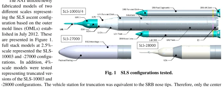
The SLS is an evolvable vehicle system consisting of a payload section, upper stage, and common core aided by two 5-segment SRBs. For the SLS-10003 Block 1 configuration, the payload section is made up of the LAS tower and MPCV. The MPCV Stage Adapter (MSA) transitions the MPCV Encapsulated Service Module (ESM) to the Interim Cryogenic Propulsion Stage (ICPS) upper stage. The ICPS transitions to the liquid oxygen (LOX) tank forward skirt via the Launch Vehicle Stage Adapter (LVSA). The SLS-27000 and -28000 Block 1B configurations replace the LVSA with a cylindrical interstage and the ICPS with the Exploration Upper Stage (EUS). The SLS-27000 Block 1B cargo variant tops the EUS with an ogive payload fairing. The SLS-28000 Block 1B crew variant tops the EUS with an Upper Stage Adapter (USA) and MPCV with LAS. For all configurations, the core consists of LOX tank and liquid hydrogen (LH2) tanks separated by an intertank. The engine section (ES) with four RS-25 engines are at the base of the LH2 tank. The left and right SRBs attach at the intertank and ES. Both SRBs consist of five solid fuel segments capped with a cylindrical forward skirt and conical nose. A conical aft skirt and nozzle is downstream of the aft fuel segment. The SRB attach hardware on the SRB side is at the booster forward skirt and around the aft fuel segment via an external attach ring.

B. SLS Wind Tunnel Models

Fig. 1 SLS configurations tested. The AAT utilized newly

fabricated models of two different scales represent-ing the SLS ascent config-uration based on the outer mold lines (OMLs) estab-lished in July 2012. These are presented in Figure 1. full stack models at 2.5%-scale represented the SLS-10003 and -27000 configu-rations. In addition, 4%-scale models were tested representing truncated ver-sions of the SLS-10003 and

-28000 configurations. The vehicle station for truncation was equivalent to the SRB nose tips. Therefore, only the center body was modeled in the truncated models. Detailed descriptions and figures for the AAT models are documented by Herron et al.[2]

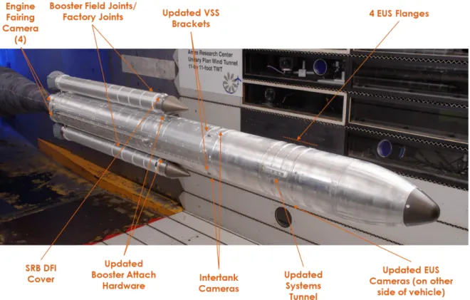
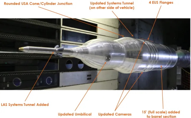
The AUAT utilized the existing AAT models, with modifications made to existing hardware or new parts machined where necessary. The AUAT was a Block 1B centric test which focused on the SLS-27005 and SLS-28005 configurations. The primary changes between those versions and the earlier -27000 and -28000, highlighted in Figures 2 and 3, were the inclusion of the intrastage adapter flanges on the EUS, updates to the EUS systems tunnel and camera geometries, modified vehicle stabilization system (VSS) bracket fairings (the VSS is used for damping wind induced oscillations during pre-launch operations), and more current camera configurations on the Core Stage forward skit adapter above the LO2 tank. These changes were all common to both the 2.5% scale full stack 27k model and the 4% scale forebody 28k model.

Each model also had a number of modifications which were specific to it. On the 2.5% model the forward attach hardware and the cameras located on Core Stage engine fairing were updated to reflect the latest design. A new hemispherical protuberance, referred to as the DFI cover, was also added on to the outboard side of the Booster forward skirts. Additionally, the previously unmodeled (but historically present) field and factory joints along the Booster segments were also incorporated for the AUAT, along with the flange which joins the top most segment with the forward

skirt. Note that the joints were only implemented on the top half of the Boosters, as a number of sensors on the lower portions of the Core Stage LH2 tank were relocated to other locations on the model for this test. These modifications are represented in Figure 2. Updates to the 4% model, shown in Figure 3 included the addition of the systems tunnel located on the Launch Abort System (LAS) tower, an updated protuberance profile for the umbilical plate located on the crew capsule ogive, and a rounded corner (as opposed to the previously sharp corner) at the USA cone to cylinder junction.

Fig. 3 Model changes for the 4% forebody Block 1B crew configuration.

Finally, in addition to the previous baseline payload fairing geometry for the SLS-27005 configuration tested for the AAT, the AUAT also included two modified fairing configurations: a tangent ogive shape with the constant diameter start point occurring 40% of the way down the fairing from the tip (as opposed to 60% for the original baseline), as well as a biconic shape with the same transition point at 40% of the length. These are displayed in Figure 4.

The models were designed by Donald Morr of Millennium Engineering and Integration Company located at NASA ARC, based on the MSFC-provided computer aided design files of the full scale vehicle. Fabrication and transducer installation were performed by MicroCraft, Inc., in Tullahoma, TN. A number of the flanges and protuberances added on for the AUAT were produced by the additive manufacturing lab at MSFC and LaRC.

(a) Tangent Ogive (b) Biconic Fig. 4 2.5% full stack Model alternative payload fairings.

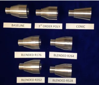
Fig. 5 Interchangeable fairing configurations for USA Trade Study conducted at MSFC TWT. The MSFC TWT test article was a 0.6%-scale model of

the Block 1B crew vehicle with seven separate USA con-figurations. Each USA section was 2.362 inches in length and machined from 6061-T6 aluminum. These included the baseline sharp corner configuration, a hypothetical configu-ration which utilized a 3rd order polynomial for the conical section, a straight conic configuration, and a series of blended configurations which employed varying radii on the shoulder. These are displayed in Figure 5.

III. Instrumentation

The models were instrumented with high frequency pres-sure transducers and were placed to capture the range of know unsteady phenomena. A limited set of unsteady CFD solutions was also utilized for the AUAT to place additional sensors in locations of interest. Planar projections showing instrumentation locations and major protuberances for each configuration tested are given in Figures 7 and 8, which depict relative proximity to the protuberances represented by approximate block shapes. The structural coordinate system clocking angle (φsc) is shown.

A. High Frequency Pressure Transducers

The AUAT models were instrumented with a total of 386 unsteady Kulite®Semiconductor Inc. ultraminiature transducers. These were distributed across all configurations as specified in Table 1. Models XCL-072-5D and -15D differential transducers and XCL-072-15A absolute transducers were used for acquiring aeroacoustic data.

Fig. 6 B-screen transducer holder used for most dynamic measurements. To minimize broadband noise induced by the transducer being out of flush

with the model OML, the transducers were installed via holders. The holders were individually contoured to the model surface prior to transducer installation to ensure flush mounting. The majority of the holders were based on a Kulite B-screen design, consisting of ten equally spaced 0.008 in. diameter holes in a 0.048 in. diameter circle, as shown in Figure 6. This design has been shown to minimize cavity noise induced by holders used in past NASA testing[3].

For the most part all of the AAT sensor locations were re-used for the AUAT, with the exception of 30 core stage/engine section sensors which were not re-instrumented due to limited space on the sting. Additionally, a small number of the AAT sensors located on the Core Stage for both tests

did not utilize the B-screens but instead implemented a single-hole design. Additional details on AAT sensor layouts, as well as specifications for the Kulite®single-hole holder designs, can be found in [2].

Table 1 SLS AUAT Instrumentation Allocation.

Model Dynamic Transducers Static Pressure

Measurements

SLS-27005 common, 2.5% full stack 248 82

SLS-27005 baseline fairing, 2.5% full stack 37 22

SLS-27005 alt. tangent ogive fairing, 2.5% full stack 57 0

SLS-27005 alt. biconic fairing, 2.5% full stack 57 0

(a) Baseline cargo fairing with common core.

(b) Left hand SRB.

(c) Alternate tangent ogive cargo

fairing. (d) Alternate biconic cargo fairing.

Fig. 7 SLS Block 1B 2.5% full stack cargo configuration model instrumentation.

Fig. 8 SLS Block 1B 4% forebody crew configuration model instrumentation.

B. Visualization

Shadowgraph photographs and movies were obtained for the points during pitch polars on the AAT and AUAT. The viewing window was limited and adjusted for each configuration to capture areas of interest, such as the cone to cylinder transition points on the payload shrouds and stage adapters, as well as major protuberances.

The TWT 0.6% forebody model used for the USA Trade Study was not instrumented with pressure sensors due to the model size and cost. The study was done using high-speed schlieren captured using a Vision Research Phantom

V1910 and a 700mm Lens, an LED strobe, and the facilities’ mirrors with knife edge. The high speed schlieren camera was triggered for a 1 second burst and a frame rate of 16k frames per second for the majority of the runs. For a select run sequences studies were conducted using higher frame rates, up to 49 fps, however the higher frame rate did not produce significant gains, and created data lags. Videos were viewed after each run and cut down to .cine files of around 100 frames in order to minimize the time between runs that was needed for the camera to download files to a local computer.

IV. Facility Information

The UPWT at ARC are a set of three interconnected tunnels that share a central main drive system that can be used to drive either a transonic leg (11’ x 11’) or a supersonic leg (9’ x 7’), as shown in Figure 9. The third high speed leg is the supersonic 8’x7’ test section, which is in mothball status and cannot currently be utilized. The 11’x11’ transonic section is a closed-return variable-density tunnel with a fixed geometry, ventilated test section, and a dual-jack flexible nozzle. The test section has 5.6% porosity consisting of evenly distributed slots on all four walls. Air flow is produced by a three-stage, axial-flow compressor powered by four wound-rotor variable-speed induction motors. The Mach number range is 0.20 to 1.50 with Reynolds number varying from 0.3- to 9.6-million per foot.

Fig. 10 MSFC TWT Layout. The 9’x7’ supersonic section is also a closed-return

variable-density tunnel, but is equipped with an asymmetric sliding block nozzle. The test section Mach number can be varied by translating the fixed contour block that forms the floor of the nozzle in the stream-wise direction. Airflow is produced by an 11-stage, axial-flow compressor powered by the same four wound-rotor variable-speed induction motors used for the 11’x11’. The Mach number range is 1.54 to 2.56 with Reynolds number variation from 0.9- to 6.5-million per foot.

The NASA MSFC ARF TWT is an intermittent, blow-down wind tunnel that operates from high-pressure storage to either atmospheric or vacuum exhaust. It was designed and constructed from 1954 through 1955 and has been functional since early 1957. Both of the TWT’s interchangeable test sections (Figure 10) measure 14 x 14 inches. The transonic test section provides a Mach number range from 0.2 to 2.5. Airspeed is varied in the subsonic range (Mach 0.2 to 0.85) by a controllable diffuser; in the transonic range (Mach 0.9 to 1.3) by auxiliary plenum suction and perforated walls, which also allow for reflected shockwave cancellation; and in the lower supersonic range

using nozzle blocks to achieve discrete Mach numbers, namely 1.46, 1.69, 1.96, and 2.5. The supersonic test section provides a Mach number range from 2.74 to 4.96. Airspeed is varied in the higher supersonic range in approximately 0.25 Mach number increments by rotating and translating fixed contour plates positioned by electric-motor screw jacks that set the nozzle and test section throat areas.

The TWT has an automated hydraulic sector that pitches between nominally±9.5◦total angles of attack. Various offsets can be installed to achieve higher total angles of attack while still remaining within sector limits. The TWT currently has no automated roll mechanism. Therefore, roll angle changes must be performed manually. To facilitate roll and configuration changes, the pitch sector and diffuser telescope to allow access to the test section and model.

V. Operations

A. Test Operations

Tests at the Ames UPWT consisted of a series of pitch or yaw polars in both the transonic and supersonic test sections for the so-called cardinal Mach numbers. Mach sweeps were also performed atα, β= 0◦to increase the chances of observing the peaks levels of the most transient phenomena. Data were only obtained once the conditions had stabilized within specified residual tolerances, given in Table 2. For the AAT the transducer sample rates were 153.6 kHz and 102.4 kHz for the 2.5% and the 4% models respectively. For the AUAT sample rates were 200kHz for both models.

Table 2 Residual Tolerances for Stabilized Tunnel Condition

Variable Tolerance

Mach ±0.005

Total Pressure ±5 psf Total Temperature ±5◦Rankine Reynolds Number ±5x1041/foot

Pitch/Yaw ±0.25◦ Simultaneous acquisition across all dynamic channels was accomplished

using National Instruments PXI based hardware and several computers running Windows® XP. All collection computers were connected to PXI-1045 chassis via MXI-2 PXI-8360 interface cards. The data system coordinator (DSC) used seven PXI-6652 timing and routing cards. One PXI-6652 card generated the master acquisition clock and triggers, and the other six distributed the signals to each of the acquisition chassis. Data acquisition was triggered by the DSC computer when the wind tunnel systems indicated that freestream and model position conditions were achieved, as in Table 2. Data acquisition triggers were received by the PXI 6652 timing cards located in each of the acquisition chassis. Data were digitized using PXI 4462 24-bit A/D cards capable of 204x103samples per second.

At the MSFC TWT data were acquired in the point-pause mode of

operation at discrete angles of attack. Once the model arrived on point, the high speed schlieren camera triggered for a 1 second burst and a frame rate of 16k frames per second. Each configuration was achieved by interchanging the mid-sections attached to the truncated common core section and the LAS/MPCV assembly. A limited set of runs were also obtained for some experiments involving an increased frame rate to 49k frames per second. This was then repeated

for a "pseudo-sweep" mode of operation wherein continuous video coverage was obtained over a large sector range. A run condition summary for both UPWT tests and the TWT test is presented in Table 3.

Table 3 Run Condition Summary

Test Mach α β AAT 0.7, 0.8, 0.85, 0.9, 0.95, 1.05, 1.10, 1.20, 1.40, 1.55, 1.75, 2.00, 2.25, and 2.50 0◦,±1◦,±2◦,±4◦,±6◦ 0◦,±2◦,±4◦,±6◦ Sweep, 0.8 – 1.4, increment of 0.01 0◦ 0◦ Sweep, 1.55 – 2.0, increment of 0.02 0◦ 0◦ AUAT 0.7, 0.8, 0.85, 0.9, 0.95, 1.05, 1.10, 1.20, 1.40, 1.55, 1.75, 2.00, 2.25, and 2.50 0◦,±1◦,±2◦,±2.83◦,±4◦, ±₆◦ 0◦,±1◦,±2◦,±2.83◦, ±₄◦_,±₆◦ Sweep, 0.7 – 1.4, increment of 0.01 0◦ 0◦ Sweep, 1.55 – 2.0, increment of 0.02 0◦ 0◦ USA Trade 0.8, 0.9, 0.95, 1.0, 1.05, 1.1, 1.15, 1.2, 1.25, 1.3 0◦,±2◦,±4◦,±6◦,±8◦,±9.5◦ 0◦

B. Calibration and Health Checks

Transducer health checks and phase-matching were performed by ARC. No static calibrations were performed on the unsteady pressure transducers. All static health checks and data processing used factory-supplied calibration for each transducer. All transducers underwent a static health check that included twelve calibration pressures. For each calibration point a known pressure was applied to the measurement side of the diaphragm. This procedure was performed in a laboratory setting with groups of eight transducers. Static health checks were also performed several times during the test. During in-situ static health checks, the reference pressure was set to several known pressures. Results of the in-situ static health checks were tracked to document transducer health. Transducers that showed output variation of more than 0.5 decibels (dB referenced to 20x10−6pascals) and of more than 1.0 dB were noted as a bad static health check. Repeated cases of greater than 1.0 dB indicate a damaged transducer. Also, to verify the health, operation, and validity of the static pressure modules and the dynamic transducers, measurements were taken with no flow at tunnel pressure conditions after the tunnel was sealed and before the tunnel was opened. Data quality checks were also performed by comparing groupings of sensors which were expected to produce similar responses. Sensors identified as significantly out-of-family were removed from the results. Across the AAT and AUAT, overall attrition was around 4%.

VI. Data Analysis

A. Dynamic Data Analysis

Data processing was done largely using MATLAB®. Data were delivered in the form of pressure time histories in native counts. Data were converted to voltage from the data acquisition system native format and then to engineering units, taking into account amplifier gain using scaling, offset, gain, and calibration coefficients in data acquisition scripts provided by ARC. Because this analysis is concerned only with the fluctuating pressure component of the time history, the static component of the time history data was removed. This was accomplished by detrending, which removes linear trends from a dataset. This process tares the time history data so that pressure data fluctuates about a zero rather than some non-zero static pressure. The data were then Fourier-analyzed to provide power spectral density (PSD) spectra that could be converted to narrowband aeroacoustic spectra using the MATLAB®functionpwelch(). All frequencies above a Nyquist cutoff of the sample rate divided by 2 were removed from the analysis. PSDs were converted to narrowband

in dB using Equation 1, whereLp,M Sis the model scale narrowband FPL in dB, andPr e f is the reference pressure, 20x10−6pascals. Lp,M S=10 log10 PSD∗SampleRate/Window P2 r e f ! (1) Corrections to the data were done in model scale. Tunnel noise was removed using empty tunnel acoustic surveys of the UPWT test sections[5]. Sources of tunnel noise included the compressor, strut, and wall slots in the 11’x11’ and compressor in the 9’x7’. High frequency tones due to transducer mount induced noise from the single-hole holder transducers were also removed. Shock reflections off the 9’x7’ walls and ceiling were taken into account. Location of OML impingement was estimated per recommendations of the tunnel user guide[4], and all measurements aft of a shock reflection impingement were ignored. Bad runs and measurements were also removed. These points were identified using health checks throughout the test, and also by time history review post-test. Data were scaled to full scale using the SLS Ascent Aeroacoustic Design Trajectory[6]. Amplitude was scaled assuming the nondimensional FPL coefficient,∆Cp,r ms, at a given vehicle location in the wind tunnel is equivalent to that at full scale, as in Equations 2, wherepr msis root-mean-square acoustic pressure andq∞is free stream dynamic pressure. Using the definition of FPL in Equation 3, amplitude scales as a function of the flight-to-tunnel dynamic pressure ratio, given in Equation 4.

|∆Cp,r ms|f light =|∆Cp,r ms|tunnelwhere∆Cp,r ms= pr ms q∞ (2) F PL=20 log₁₀ pr ms pr e f (3)

F PLf light =F PLtunnel+20 log10 _q

∞,f light q∞,tunnel

(4) Frequency was scaled assuming the nondimensional Strouhal number,St, in the wind tunnel is equivalent to that at full scale, as in Equation 5 where f is frequency,lis a characteristic dimension such as diameter or length, andUis flow velocity. Therefore, frequency scales as a function of wind tunnel model scale and flight-to-tunnel velocity. Because the tunnel medium is air, at a given Mach number velocity is only a function of static temperature (T) and so frequency scales as in Equation 6.

|St|_{f light}=|St|_tunnelwhereSt= f l/U (5)

ff light = ltunnel lf light s Tf light Ttunnel ftunnel (6)

The resulting full-scale narrowband spectra were integrated to produce one-third octave bands, ranging from 10 to 2000 Hz. Full-scale overall FPL (OAFPL) levels were calculated by log summing one-third octave FPLs over the entire bandwidth.

B. Data Vizualization

In order to help visualize and interpret the dynamic data results a plotting technique was used whereby either OAFPL or∆Cp,r msvalues for each sensor are mapped onto a three dimensional representation of the vehicle model to create a rough contour plot. In order to create these plots the model CAD files are first imported into the BETA CAE Systems’ ANSA pre-processor and a coarse mesh is generated over the geometry surface. Next, they are exported as stereolithography (.stl) files and imported into MATLAB®. There, the x y and z coordinates are converted such that they can be utilized by the built-inpatch()function. The value specification for each vertex of the mesh is obtained by using thescatteredInterpolant()function, which creates a 3-D dimensional interpolant based on the sensor position and magnitude. The “nearest” technique is used to create a contour plot which has large patches of uniform color around each sensor. Both specific run conditions as well as envelopes over Mach,α, andβspace can be visualized. To compare results between the AUAT and AAT, the interpolant of the latter can be subtracted from the former to produce a∆OAFPL contour plot.

C. TWT Schlieren Analysis

Schlieren was used as the primary means of analysis for the USA trade study. Due to the large amount of noise in the images from the inherint noise of the TWT being a blow down tunnel, it was often hard to discern the images. Multiple techniques were employed in order to view the flow characteristics more clearly. These techniques include manipulation of the image in the Phantom propriety imaging software, and the use of basic edge finding techniques using MATLAB®. Using these methods schlieren were used to characterize the different geometries and the shock location and characteristics. Schlieren and shadowgraph of the tests proved to be important for subsequent testing. Images from the MSFC ARC TWT were used to fine tune instrumentation placement for the AUAT on the USA region to ensure the shock locations were captured.

VII. Results

A. USA Trade Study

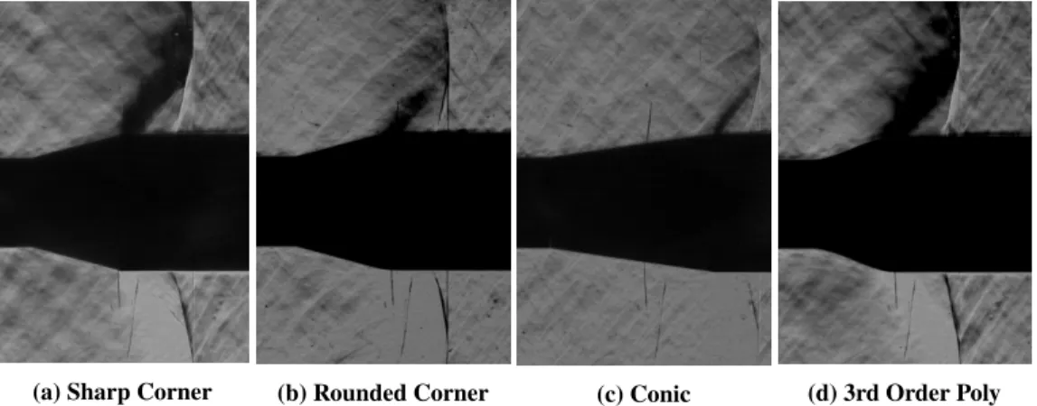
The USA Geometry study provided data on 8 different geometries. The baseline, a 3rd order polynomial curve, a conic section, and five radiused corner geometries. The most notable differences were visible at M 0.9, as shown in Figure 11. The rounded corner behaved similarly to the sharp corner, however the shock moved up and down the corner where it was stationary with the sharp corner. The conic section had a lower magnitude stationary shock. The 3rd order poynomial had favorable CFD, however appeared to indicate higher FPLs and probably higher buffet. Of the configurations tested, the selection was made to use the geometry that appeared most similar to the baseline, which was well understood, and thus would limit impacts.

(a) Sharp Corner (b) Rounded Corner (c) Conic (d) 3rd Order Poly

Fig. 11 Comparison of USA Trade Study geometries using high speed schlieren obtained at the MSFC TWT. Results for M = 0.9, andα,β= 0.

Figure 12 provides the delta OAFPL (AUAT - AAT) contour plot of sensor envelopes for the upper portion of the Block 1B crew vehicle with a negative scale . Only the sensors common to both tests we used for this plot to highlight the effect of the geometry change at the USA shoulder. The peak levels for the sharp corner shoulder used during the AAT occurred a M= 1.1, where it can be seen from the schlieren or shadowgraph image in Figure 13 that the expansion is confined to narrow region and proceeded immediately by a shock which is forming as a result of flow separation just downstream of the expansion. The rounded shoulder allows for a more gradual expansion, reducing the severity of the separation and eliminating the shock. The result is an approximate 5 dB reduction in overall fluctuating pressure level on the cylindrical section of the adapter, as evidenced by the contour plot.

Fig. 12 Delta contour plot of OAFPL values (AUAT - AAT) for envelopes over all Mach,α, andβ. Only the sensors which were common to both tests were used for this comparison.

Fig. 13 Visual comparison of the schlieren imagery obtained at the MSFC TWT on the 0.6% scale sharp shoulder model (left) with the shadowgraph imagery obtained at the ARC UPWT during the AUAT for the 4% rounded shoulder model (right). Both images are for M = 1.1 atα,β= 0

B. LAS Nozzle Wake Effects

(a) Mach 0.73 (b) Mach 0.84

Fig. 14 Effects of the LAS nozzle wakes on the shock/separated boundary layer system aft of the USA shoulder. α,β= 0 for both Mach numbers.

As the flow expands around the USA shoulder it accelerates, and at a critical freestream subsonic Mach number it becomes super-sonic. However, this region of expanded flow cannot be maintained as the pressure moving aft increases, and a normal shock wave forms which returns the flow to subsonic conditions. The shock wave is also accom-panied by a localized region of flow separation imme-diately downstream. This system produces some of the higher fluctuating pres-sure levels on this compo-nent of the vehicle. Fig-ure 14 provides contour plots of the upper portion of the Block 1B forebody configuration at α, β = 0 for Mach 0.73 and Mach 0.84. These two conditions were taken from the high fi-delity Mach sweep and cap-ture the shock as it marches downstream. A relatively dense grid of sensors was placed in this location to measure any discernible in-fluence of the turbulent fluc-tuations produced by the LAS nozzle wakes on these flow features.

The overall fluctuating

pressures for both cases exhibit about 15% variation across the wake, which is roughly equivalent to ~1.5 dB. Figure 15 provides the accompanying spectral content for each sensor. For Mach 0.73, it can be seen that the discrepancy at the peak frequency of 25 Hz is more pronounced, a roughly 25% decrease from the highest to the lowest, or ~2.5 dB. For the Mach 0.84 case the peak has shifted to 5 Hz, however the largest variation in magnitude still occurs around 25 Hz, and is around 50% decrease from highest to lowest, or ~4 to 5 dB. It is also observed that whereas in the Mach 0.73 case the minimum levels occurred at the sensor immediately downstream of the nozzle, for the Mach 0.84 case it occurs at the sensors towards the region in the middle of the nozzles.

In general it appears that the nozzle wakes are not affecting overall levels as much as they are redistributing the energy into different frequencies, with a predominant effect at 25 Hz. Interestingly though, this does not correlate with the predominant wake tone itself which occurs at ~100 Hz. The limited conditions at which the shock and separation are present, as well as the still rather course spatial resolution of the sensors, makes a more definitive observation of the wake influence difficult. However, experimental measurements were also obtained during the test using unsteady pressure sensitive paint (uPSP) [7], which allows for CFD-like spatial resolution of the entire surface in the sub 200 Hz range. At the time of writing those measurements are still being processed, but they represent an excellent opportunity to study this problem in more detail in the future.

(a) Mach 0.73 _{(b) Mach 0.84}

Fig. 15 Spectra for each sensor corresponding to the labels provided in the contour plots above

C. EUS Flange Effects

Fig. 16 Delta contour plot of OAFPL values (AUAT-AAT) at M = 1.2 andα,β= 0. Red dots indicate sensors common to both tests and white dots indicate sensors present only for the AUAT.

Figure 16 provides a contour plot of the upper portion of the Block 1B crew configuration showing the change in overall fluctuating pressure level envelopes between the two acoustics tests at the UPWT (AUAT - AAT). The red dots are indicative of sensor locations common to both tests, while the white dots are sensors that were present only for the AUAT. The envelopes are derived for each sensor from all Mach, α, and βconditions tested.The primary change to the OML between the two tests in this region was the addition of the four flanges on the EUS, where it is clearly seen that they induce an ~8 to 10 dB increase as compared to the clean skin. It is interesting to note that the topmost flange, joining the USA to the EUS forward skirt, produces an ~5 to 7 dB increase, which is characteristic of other flanges on the vehicle in isolation. However, the succession of flanges in close proximity affects the reattachment downstream of each, resulting an additional increase to the fluctuating pressure levels. This is also apparent in figure 17, which displays a pixel variance shadowgraph image of this region for Mach 1.02. The pixel variance is proportional to fluctuating pressure, where the lighter areas represent greater unsteadiness. Regions of significant flow separation can be seen be-tween flanges, which are stronger in magnitude than the separation after the last flange.

It should also be noted that a large number of the small patches and slivers of bright spots on the delta contour plot are generally in regions where sensors were added for the second test. In some cases they are picking up previously undetected hot spots or new flow features. In other cases they are simply an artifact caused by the process of subtracting two interpolation surfaces based on different sensor sets. On the whole though the subtraction technique is useful for visualizing bulk trends.

Fig. 17 Shadowgraph with pixel variance shows the regions of flow separation between flanges on the EUS. For M = 1.02 atα,β= 0.

D. Booster Rings and Multibody Effects

Figure 18 displays a contour plot of the Core Stage and the one Booster which was instrumented during testing. Figure 18a shows the enveloped fluctuating pressure coefficients for each sensor over all Mach,α, andβspace, while figure 18b provides a contour plot of the delta OAFPL between the two tests (AUAT - AAT). Note here that the∆Cp,r ms

values are calculated using the maximum dynamic pressure from the design trajectory (rather than the condition which produced the maximum value for each sensor). Again, the effect of adding flanges (in this case the segment field and factory joint rings) is significant. In this instance though, most notable is the fact that not only are the sensors on the Booster in the immediate vicinity of the rings affected, but Core Stage sensors are as well. Based on steady state CFD, as well as Space Shuttle External Tank flight imagery post separation, it is believed that the shocks emanating from the rings at supersonic conditions are impinging on the Core Stage and causing localized flow separation. This was not anticipated (as evidenced by the fact the rings were not included on earlier SLS or Space Shuttle aeroacoustics tests) due to the fact that they are roughly 1 inch tall full scale and expected to be buried in the boundary layer.

In examining the two plots further, it is observed that only the last two rings produce an increase on both the Core Stage and Booster. This is because the levels generated by the alternating wake flow coming off of the forward attach dominate in this region. If fact, these levels are the loudest recorded anywhere on the vehicle during ascent. As that feature attenuates though, the local ring induced flow separation and shock impingement begin to dominate. Interestingly, it may be the forward attach wake that is itself responsible for re-setting the boundary layer along the Booster, making it shallow enough to allow for shock formation. While the phenomenon is not yet understood in detail, the observation is illustrative in showing the importance of modeling otherwise unassuming features for aeroacoustic testing. In this instance in particular the interaction of complex flow fields produced by multiple bodies generated an unanticipated result which had non-trivial consequences for the program.

(a) Contour plot of AUAT results. Envelope over all Mach,α, andβ. All sensors common to both

tests

(b) Delta OAFPL contour plot (AUAT - AAT). Envelope over all Mach,α, andβ. All sensors

common to both tests Fig. 18 Effects of the SRB rings produced by multibody interactions.

E. Fairing Study

Figure 19 displays contour plots of all three fairings tested on the 2.5% model during the AUAT. The values are envelopes of only the high fidelity Mach sweep taken atα/β= 0. Note that all three figures utilize the same scale. The primary observation is that the peak levels for the elongated tanget ogive (or baseline configuration) which occur right at the shoulder of the fairing are about 40% greater than those recorded for cylindrical section of the other two fairings. For the short tangent-ogive it appears that the high resolution shock array may not have captured the peak value which likely occurrs closer to the shoulder. The scenario for the biconic is possibly the same, however, there is some indication that the shock may actually start farther downstream on account of the fact that the forward most ring of sensors on the cylindrical portion did not record levels comparable to the peak of the array, as was the case for the short tangent ogive. This may make sense if the magnitude of the expansion was weakened by the first. Additionally, it is observed that levels around the EUS flanges are a bit higher for both tangent ogive fairings than for the biconic. This may be due to the existence of two shocks here, one on each expansion. Due to the non-isentropic nature of shock waves the flow downstream will be at a lower total pressure for this configuration, which would result in lower magnitude pressure fluctuations.

(a) 27s baseline (b) Alt. biconic (c) Alt. tangent ogive

Fig. 19 Comparison of different cargo fairing configurations. Contour plots are envelopes of the high fidelity Mach sweeps performed atα, β= 0

VIII. Conclusions

Multiple test campaigns utilizing numerous configurations of common vehicle designs has resulted in a wealth of aeroacoustic data. In many instances small configuration changes could be utilized to examine the effects of specific flow features which are applicable to a broad range launch vehicles. Based on this general observations are as follows:

1) Rounded corners on fairings can reduce maximum loads by ~5dB.

2) Long lasting flow features produced by large protuberances towards the leading edge of the vehicle can affect the frequency content of fluctuating pressure levels significantly downstream, as in the case of LAS nozzles with the transonic shock/separated boundary layer system situated on the USA.

4) The flow features produced by multibody interactions, e.g. fall away boosters with a core stage, can produce increases in unanticipated regions. It is important in this scenario to model the geometry with the highest fidelity practical.

5) Instrumentation should be placed near the shoulder of a fairing to capture the peak fluctuating pressure levels produced by a transonic shock/separated boundary layer system.

Acknowledgments

The authors would like to thank the SLS Ascent Aeroacoustics Test Team for executing a challenging and successful test program. This includes the ARC Fluid Mechanics, Computer Systems and Instrumentation, and Operations Branches. The test also required extra help for in-situ data analysis and measurement health monitoring from both the Aerodynamics and Aerothermodynamics Teams in EV33, as well as the MSFC Fluids Dynamics Branch and the LaRC Aeroelasticity Branch. The authors would also like to thank EV33 and SLS management for support.

References

[1] “Ares I Acoustic Environments Data Book,” NASA CxP 72164, 2009.

[2] Herron, A., Reed, D., and Nance, D., “Overview of the Space Launch Sytem Ascent Aeroacoustic Environment Test Program,”

54th AIAA Aerospace Sciences Meeting, AIAA, 2016.

[3] Herron, A., Reed, D., and Nance, D., “Reducing the Effect of Transducer Mount Induced Noise on Aeroacoustic Wind Tunnel Testing Data with a New Transducer Mount Design,”21st AIAA/CEAS Aeroacoustics Conference, AIAA, 2015.

[4] “Test Planning Guide for High Speed Wind Tunnels,” NASA Ames Research Center, Report Number A027-9391-XB2, Revision 5, April 2005.

[5] Amaya, M., and Richey, C., “Preliminary Data Transmittal for the 11-ft Acoustics Survey Test (Test Number 11-0196) conducted in the Ames Research Center 11-Ft. TWT,” , October 2008.

[6] Dukeman, G., “Space Launch System Aeroacoustic Design Environment Development,” NASA/MSFC EV42-14-004, September 2014.

[7] Sellers, M. E., Nelson, M. A., Burnside, N. J., and Roozeboom, N., “Evaluation of Unsteady Pressure Sensitive Paint Use for Space Launch Vehicle Buffet Determination,”55th AIAA Aerospace Sciences Meeting, AIAA SciTech Forum, AIAA, 2017.