Communication Steps for Parallel Query Processing

(1)

Communication Steps for Parallel Query Processing

∗

Paul Beame, Paraschos Koutris and Dan Suciu

University of Washington, Seattle, WA

{beame,pkoutris,suciu}@cs.washington.edu

ABSTRACT

We consider the problem of computing a relational queryq

on a large input database of sizen, using a large number

pof servers. The computation is performed inrounds, and each server can receive onlyO(n/p1−ε) bits of data, where

ε ∈ [0,1] is a parameter that controls replication. We ex-amine how many global communication steps are needed to computeq. We establish both lower and upper bounds, in two settings. For a single round of communication, we give lower bounds in the strongest possible model, where arbi-trary bits may be exchanged; we show that any algorithm re-quiresε≥1−1/τ∗, whereτ∗is the fractional vertex cover of the hypergraph ofq. We also give an algorithm that matches the lower bound for a specific class of databases. For mul-tiple rounds of communication, we present lower bounds in a model where routing decisions for a tuple are tuple-based. We show that for the class oftree-likequeries there exists a tradeoff between the number of rounds and the space expo-nentε. The lower bounds for multiple rounds are the first of their kind. Our results also imply that transitive closure cannot be computed inO(1) rounds of communication.

Categories and Subject Descriptors

H.2.4 [Systems]: Parallel Databases

Keywords

Parallel Computation, Lower Bounds

1. INTRODUCTION

Most of the time spent in big data analysis today is allo-cated in data processing tasks, such as identifying relevant data, cleaning, filtering, joining, grouping, transforming, ex-tracting features, and evaluating results [5, 8]. These tasks form the main bottleneck in big data analysis, and a ma-jor challenge for the database community is improving the

∗

This work was partially supported by NSF IIS-1115188, IIS-0915054 and IIS-1247469.

Permission to make digital or hard copies of all or part of this work for personal or classroom use is granted without fee provided that copies are not made or distributed for profit or commercial advantage and that copies bear this notice and the full citation on the first page. To copy otherwise, to republish, to post on servers or to redistribute to lists, requires prior specific permission and/or a fee.

performance and usability of data processing tools. The mo-tivation for this paper comes from the need to understand the complexity of query processing in big data management. Query processing is typically performed on a shared-nothing parallel architecture. In this setting, the data is stored on a large number of independent servers interconnected by a fast network. The servers perform local computations, then exchange data in global data shuffling steps. This model of computation has been popularized by MapReduce [7] and Hadoop [15], and can be found in most big data processing systems, like PigLatin [21], Hive [23], Dremmel [19].

Unlike traditional query processing, the complexity is no longer dominated by the number of disk accesses. Typically, a query is evaluated by a sufficiently large number of servers such that the entire data can be kept in the main memory of these servers. The new complexity bottleneck is the commu-nication. Typical network speeds in large clusters are 1Gb/s, which is significantly lower than main memory access. In addition, any data reshuffling requires a global synchroniza-tion of all servers, which also comes at significant cost; for example, everyone needs to wait for the slowest server, and, worse, in the case of a straggler, or a local node failure, ev-eryone must wait for the full recovery. Thus, the dominating complexity parameters in big data query processing are the number of communication steps, and the amount of data being exchanged.

MapReduce-related models.

Several computation models have been proposed in order to understand the power of MapReduce and related mas-sively parallel programming methods [9, 16, 17, 1]. These all identify the number of communication steps/rounds as a main complexity parameter, but differ in their treatment of the communication.

The first of these models was the MUD (Massive, Un-ordered, Distributed) model of Feldman et al. [9]. It takes as input a sequence of elements and applies a binary merge operation repeatedly, until obtaining a final result, similarly to a User Defined Aggregate in database systems. The paper compares MUD with streaming algorithms: a streaming al-gorithm can trivially simulate MUD, and the converse is also possible if the merge operators are computationally powerful (beyond PTIME).

Karloff et al. [16] defineMRC, a class of multi-round al-gorithms based on using the MapReduce primitive as the sole building block, and fixing specific parameters for bal-anced processing. The number of processorspis Θ(N1−), and each can exchange MapReduce outputs expressible in Θ(N1−) bits per step, resulting in Θ(N2−2) total storage

(2)

among the processors on a problem of sizeN. Their focus was algorithmic, showing simulations of other parallel mod-els byMRC, as well as the power of two round algorithms for specific problems.

Lower bounds for the single round MapReduce model are first discussed by Afrati et al. [1], who derive an interesting tradeoff between reducer size and replication rate. This is nicely illustrated by Ullman’s drug interaction example [25]. There aren(= 6,500) drugs, each consisting of about 1MB of data about patients who took that drug, and one has to find all drug interactions, by applying a user defined func-tion (UDF) to all pairs of drugs. To see the tradeoffs, it helps to simplify the example, by assuming we are giventwo

sets, each of sizen, and we have to apply a UDF to every pair of items, one from each set, in effect computing their cartesian product. There are two extreme ways to solve this. One can usen2 _{reducers, one for each pair of items; while}

each reducer has size 2, this approach is impractical because the entire data is replicatedntimes. At the other extreme one can use a single reducer that handles the entire data; the replication rate is 1, but the size of the reducer is 2n, which is also impractical. As a tradeoff, partition each set intoggroups of sizen/g, and use one reducer for each of the

g2 _{pairs of groups: the size of a reducer is 2}_n/g_{, while the}

replication rate isg. Thus, there is a tradeoff between the replication rate and the reducer size, which was also shown to hold for several other classes of problems [1].

Towards lower bound models.

There are two significant limitations of this prior work: (1) As powerful and as convenient as the MapReduce frame-work is, the operations it provides may not be able to take full advantage of the resource constraints of modern sys-tems. The lower bounds say nothing about alternative ways of structuring the computation that send and receive the same amount data per step. (2) Even within the MapRe-duce framework, the only lower bounds apply to a single communication round, and say nothing about the limita-tions of multi-round MapReduce algorithms.

While it is convenient that MapReduce hides the num-ber of servers from the programmer, when considering the most efficient way to use resources to solve problems it is natural to expose information about those resources to the programmer. In this paper, we take the view that the num-ber of serverspshould be an explicit parameter of the model, which allows us to focus on the tradeoff between the amount of communication and the number of rounds. For example, going back to our cartesian product problem, if the number of serverspis known, there is one optimal way to solve the problem: partition each of the two sets intog=√pgroups, and let each server handle one pair of groups.

A model with p as explicit parameter was proposed by Koutris and Suciu [17], who showed both lower and upper bounds for one round of communication. In this model only tuples are sent and they must be routed independent of each other. For example, [17] proves that multi-joins on the same attribute can be computed in one round, while multi-joins on different attributes, likeR(x), S(x, y), T(y) require strictly more than one round. The study was mostly focused on understanding data skew, the model was limited, and the results do not apply to more than one round.

In this paper we develop more general models, establish lower bounds that hold even in the absence of skew, and use

a bit model, rather than a tuple model, to represent data.

Our lower bound models and results.

We define theMassively Parallel Communication(MPC) model, to analyze the tradeoff between the number of rounds and the amount of communication required in a massively parallel computing environment. We include the number of servers p as a parameter, and allow each server to be in-finitely powerful, subject only to the data to which it has access. The model requires that each server receives only

O(N/p1−ε) bits of data at any step, whereN is the prob-lem size, andε ∈ [0,1] is a parameter of the model. This implies that the replication factor is O(pε_{) per round. A}

particularly natural case is ε = 0, which corresponds to a replication factor ofO(1), orO(N/p) bits per server;ε= 1 is degenerate, since it allows the entire data to be sent to every server.

We establish both lower and upper bounds for comput-ing a full conjunctive query q, in two settings. First, we restrict the computation to a single communication round and examine the minimum parameterεfor which it is possi-ble to computeqwithO(N/p1−ε) bits per processor; we call this thespace exponent. We show that the space exponent for connected queries is always at least 1−1/τ∗(q), where

τ∗(q) is the fractional (vertex) covering number of the hy-pergraph associated withq[6], which is the optimal value of the vertex cover linear program (LP) for that hypergraph. This lower bound applies to the strongest possible model in which servers can encode any information in their messages, and have access to a common source of randomness. This is stronger than the lower bounds in [1, 17], which assume that the units being exchanged are tuples.

Our one round lower bound holds even in the special case of matching databases, when all attributes are from the same domain [n] and all input relations are (hypergraph) matchings, in other words, every relation has exactly n

tuples, and every attribute contains every value 1,2, . . . , n

exactly once. Thus, the lower bound holds even in a case in which there is no data skew. We describe a simple tuple-independent algorithm that is easily implementable in the MapReduce framework, which, in the special case of matching databases, matches our lower bound for any conjunctive query. The algorithm uses the optimal solution for the fractional vertex cover to find an optimal split of the input data to the servers. For example, the linear query

L2 = S1(x, y), S2(y, z) has an optimal vertex cover 0,1,0

(for the variablesx, y, z), hence its space exponent isε= 0, whereas the cycle query C3 = S1(x, y), S2(y, z), S3(z, x)

has optimal vertex cover 1/2,1/2,1/2 and space exponent

ε = 1/3. We note that recent work [13, 4, 20] gives upper bounds on the query size in terms of a fractionaledge cover, while our results are in terms of thevertex cover. Thus, our first result is:

Theorem 1.1. For every connected conjunctive query q, anyp-processor randomized MPC algorithm computingq in one round requires space exponent ≥ 1−1/τ∗(q). This lower bound holds even over matching databases, for which it is optimal.

Second, we establish lower bounds for multiple communi-cation steps, for a restricted version of the MPC model, called tuple-based MPC model. The messages sent in the first round are still unrestricted, but in subsequent rounds the servers can send only tuples, either base tuples in the

(3)

in-put tables, or join tuples corresponding to a subquery; more-over, the destinations of each tuple may depend only on the tuple content, the message received in the first round, the server, and the round. We note that any multi-step MapRe-duce program is tuple-based, because in any map function the key of the intermediate value depends only on the input tuple to the map function. Here, we prove that the number of rounds required is, essentially, given by the depth of a query plan for the query, where each operator is a subquery that can be computed in one round for the given ε. For example, to compute a length k chain query Lk, ifε = 0, the optimal computation is a bushy join tree, where each operator isL2 (a two-way join) and the optimal number of

rounds is log₂k. If ε= 1/2, then we can useL4 as

opera-tor (a four-way join), and the optimal number of rounds is log4k. More generally, we can show nearly matching upper

and lower bounds based on graph-theoretic properties of the query such as the following:

Theorem 1.2. For space exponentε, the number of rounds required for any tuple-based MPC algorithm to compute any tree-like conjunctive queryqis at leastdlogkε(diam(q))ewhere kε= 2b1/(1−ε)cand diam(q) is the diameter ofq. More-over, for any connected conjunctive queryq, this lower bound is nearly matched (up to a difference of essentially one round) by a tuple-based MPC algorithm with space exponentε.

These are the first lower bounds that apply to multiple rounds of MapReduce. Both lower bounds in Theorem 1.1 and Theorem 1.2 are stated in a strong form: we show that any algorithm on the MPC model retrieves only a 1/pΩ(1)

fraction of the answers to the query in expectation, when the inputs are drawn uniformly at random (the exponent depends on the query and onε); Yao’s Lemma [26] imme-diately implies a lower bound for any randomized algorithm over worst-case inputs. Notice that the fraction of answers gets worse as the number of servers p increases. In other words, the more parallelism we want, the worse an algo-rithm performs, if the number of communication rounds is bounded.

Related work in communication complexity.

The results we show belong to the study of communi-cation complexity, for which there is a very large body of existing research [18]. Communication complexity considers the number of bits that need to be communicated between cooperating agents in order to solve computational prob-lems when the agents have unlimited computational power. Our model is related to the so-called number-in-hand party communication complexity, in which there are multi-ple agents and no shared information at the start of commu-nication. This has already been shown to be important to understanding the processing of massive data: Analysis of number-in-hand (NIH) communication complexity has been the main method for obtaining lower bounds on the space required for data stream algorithms (e.g. [3]).

However, there is something very different about the re-sults that we prove here. In almost all prior lower bounds, there is at least one agent that has access to all communica-tion between agents1. (Typically, this is either via a shared blackboard to which all agents have access or a referee who

1

Though private-messages models have been defined before, we are aware of only two lines of work where lower bounds make use of the fact that no single agent has access to all

receives all communication.) In this case, no problem onN

bits whose answer isM bits long can be shown to require more thanN+M bits of communication.

In our MPC model, all communication between servers is privateand we restrict the communication per processor per step, rather than the total communication. Indeed, the privacy of communication is essential to our lower bounds, since we prove lower bounds that apply when the total com-munication is much larger thanN+M. (Our lower bounds for some problems apply when the total communication is as large asN1+δ_.)

2. PRELIMINARIES

2.1 Massively Parallel Communication

We fix a parameterε ∈[0,1], called the space exponent, and define the MPC(ε) model as follows. The computation is performed by p servers, called workers, connected by a complete network of private channels. The input data has sizeN bits, and is initially distributed evenly among thep

workers. The computation proceeds in rounds, where each round consists of local computation at the workers inter-leaved with global communication. The complexity is mea-sured in the number of communication rounds. The servers have unlimited computational power, but there is one im-portant restriction: at each round, a worker may receive a total of onlyO(N/p1−ε) bits of data from all other workers combined. Our goal is to find lower and upper bounds on the number of communication rounds.

The space exponent represents the degree of replication during communication; in each round, the total amount of data exchanged is O(pε_{) times the size of the input data.}

When ε = 0, there is no replication, and we call this the basic MPC model. The case ε = 1 is degenerate because each server can receive the entire data, and any problem can be solved in a single round. Similarly, for any fixed ε, if we allow the computation to run for Θ(p1−ε) rounds, the entire data can be sent to every server and the model is again degenerate.

We denoteMuvr the message sent by serveruto serverv

during round r and denoteMvr = (Mvr−1,(M1rv, . . . , Mpvr ))

the concatenation of all messages sent to vup to roundr. AssumingO(1) rounds, each messageMvr holdsO(N/p

1−ε

) bits. For our multi-round lower bounds in Section 4, we will further restrict what the workers can encode in the messages

Mr

uvduring rounds r≥2.

2.2 Randomization

The MPC model allows randomization. The random bits are available to all servers, and are computed independently of the input data. The algorithm may fail to produce its out-put with a small probabilityη >0, independent of the input. For example, we use randomization for load balancing, and communication: (1) Results of [11, 14] use the assumption that communication is both private and (multi-pass) one-way, but unlike the bounds we prove here, their lower bounds are smaller than the total input size; (2) Tiwari [24] de-fined a distributed model of communication complexity in networks in which in input is given to two processors that communicate privately using other helper processors. How-ever, this model is equivalent to ordinary public two-party communication when the network allows direct private com-munication between any two processors, as our model does.

(4)

abort the computation if the amount of data received dur-ing a communication would exceed theO(N/p1−ε) limit, but this will only happen with exponentially small probability.

To prove lower bounds for randomized algorithms, we use Yao’s Lemma [26]. We first prove bounds fordeterministic

algorithms, showing that any algorithm fails with probabil-ity at leastηover inputs chosen randomly from a distribu-tionµ. This implies, by Yao’s Lemma, that every random-ized algorithm with the same resource bounds will fail on some input (in the support ofµ) with probability at leastη

over the algorithm’s random choices.

2.3 Conjunctive Queries

In this paper we consider a particular class of problems for the MPC model, namely computing answers to conjunctive queries over an input database. We fix an input vocabulary

S1, . . . , S`, where each relation Sj has a fixed arityrj; we

denoter=P`_j₌₁rj. The input data consists of one relation instance for each symbol. We denotenthe largest number of tuples in any relationSj; then, the entire database instance can be encoded usingN=O(nlogn) bits, because`=O(1) andrj=O(1) forj= 1, . . . , `.

We consider full conjunctive queries (CQs) without self-joins, denoted as follows:

q(x1, . . . , xk) =S1(¯x1), . . . , S`(¯x`) (1)

The query isfull, meaning that every variable in the body appears the head (for exampleq(x) = S(x, y) is not full), andwithout self-joins, meaning that each relation nameSj

appears only once (for exampleq(x, y, z) = S(x, y), S(y, z) has a self-join). Thehypergraphof a queryqis defined by in-troducing one node for each variable in the body and one hy-peredge for each set of variables that occur in a single atom. We say that a conjunctive query is connectedif the query hypergraph is connected (for example,q(x, y) =R(x), S(y) is not connected). We use vars(Sj) to denote the set of vari-ables in the atom Sj, and atoms(xi) to denote the set of atoms wherexioccurs;k and`denote the number of vari-ables and atoms inq, as in (1). Theconnected components

of q are the maximal connected subqueries of q. Table 1 illustrates example queries used throughout this paper.

We consider two query evaluation problems. In Join-Reporting, we require that all tuples in the relation de-fined byq be produced. In_Join-Witness, we require the production of at least one tuple in the relation defined by

q, if one exists;Join-Witnessis the verified version of the natural decision problem_{Join-NonEmptiness}.

Characteristic of a Query.

The characteristic of a conjunctive query q as in (1) is defined asχ(q) =k+`−P

jrj−c, wherekis the number of

variables,`is the number of atoms,rj is the arity of atom

Sj, andcis the number of connected components ofq. For a query q and a set of atoms M ⊆atoms(q), define

q/Mto be the query that results from contracting the edges in the hypergraph ofq. As an example, for the queryL5 in

Table 1,L5/{S2, S4}=S1(x1, x2), S3(x2, x4), S5(x4, x6).

Lemma 2.1. The characteristic of a queryq satisfies the following properties:

(a) If q1, . . . , qc are the connected components of q, then

χ(q) =Pc_i₌₁χ(qi).

(b) For anyM⊆atoms(q),χ(q/M) =χ(q)−χ(M).

(c) χ(q)≤0.

(d) For anyM ⊆atoms(q),χ(q)≤χ(q/M).

Proof. Property (a) is immediate from the definition of

χ, since the connected components of q are disjoint with respect to variables and atoms. Sinceq/M can be produced by contracting according to each connected component of

M in turn, by property (a) and induction it suffices to show that property (b) holds in the case that M is connected. If a connected M has kM variables, `M atoms, and total arity rM, then the query after contraction, q/M, will have the same number of connected components, kM −1 fewer variables, and the terms for the number of atoms and total arity will be reduced by `M −rM for a total reduction of

kM +`M−rM −1 =χ(M). Thus, property (b) follows. By property (a), it suffices to prove (c) when q is con-nected. Ifq is a single atom thenχ(q)≤0, since the num-ber of variables is at most the arity of the atom inq. We reduce to this case by repeatedly contracting the atoms of

q until only one remains and showing thatχ(q)≤χ(q/Sj): Let m ≤ rj be the number of distinct variables in atom

Sj. Then,χ(q/Sj) = (`−1) + (k−m+ 1)−(r−rj)−1 =

χ(q)+(rj−m)≥χ(q). Property (d) also follows by the com-bination of property (b) and property (c) applied toM.

Finally, let us call a query q tree-like if q is connected and χ(q) = 0. For example, the query Lk is tree-like, and so is any query over a binary vocabulary whose graph is a tree. Over non-binary vocabularies, any tree-like query is acyclic, but the converse does not hold:

q=S1(x0, x1, x2), S2(x1, x2, x3) is acyclic but not tree-like.

An important property of tree-like queries is that every connected subquery will be also tree-like.

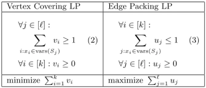
Vertex Cover and Edge Packing.

Afractional vertex cover of a queryq is any feasible so-lution of the LP shown on the left of Fig. 1. The vertex cover associates a non-negative numberui to each variable

xi s.t. every atom Sj is “covered”, P

i:xi∈vars(Sj)vi ≥ 1.

The dual LP corresponds to afractional edge packing prob-lem (also known as a fractional matching problem), which associates non-negative numbersuj to each atomSj. The two LPs have the same optimal value of the objective func-tion, known as thefractional covering number[6] of the hy-pergraph associated with q and denoted by τ∗(q). Thus,

τ∗(q) = minP

ivi = max P

juj. Additionally, if all

in-equalities are satisfied as in-equalities by a solution to the LP, we say that the solution istight.

For a simple example, a fractional vertex cover of the query2 L3 = S1(x1, x2), S2(x2, x3), S3(x3, x4) is any solu-2_{We drop the head variables when clear from the context.}

Vertex Covering LP Edge Packing LP

∀j∈[`] : X i:xi∈vars(Sj) vi≥1 (2) ∀i∈[k] :vi≥0 ∀i∈[k] : X j:xi∈vars(Sj) uj≤1 (3) ∀j∈[`] :uj≥0 minimize Pk_i₌₁vi maximize P`_j₌₁uj

Figure 1: The vertex covering LP of the hypergraph of a queryq, and its dual edge packing LP.

(5)

tion tov1+v2≥1,v2+v3≥1 andv3+v4≥1; the optimal

is achieved by (v1, v2, v3, v4) = (0,1,1,0), which is not tight.

An edge packing is a solution to u1 ≤ 1, u1 +u2 ≤ 1,

u2+u3 ≤ 1 and u3 ≤ 1, and the optimal is achieved by

(1,0,1), which is tight.

The fractional edgepacking should not be confused with the fractional edgecover, which has been used recently in several papers to prove bounds on query size and the running time of a sequential algorithm for the query [4, 20]; for the results in this paper we need the fractional packing. The two notions coincide, however, when they are tight.

2.4 Input Servers

We assume that, at the beginning of the algorithm, each relation Sj is stored on a separate server, called an input server, which during the first round sends a messageM1

juto

every workeru. After the first round, the input servers are no longer used in the computation. All lower bounds in this paper assume that the relations Sj are given on separate input servers. All upper bounds hold for either model.

The lower bounds for the model with separate input servers carry over immediately to the standard MPC model, because any algorithm in the standard model can be simulated in the model with separate input servers. Indeed, the algorithm must compute the output correctly for any initial distribu-tion of the input data on thepservers: we simply choose to distribute the input relations S1, . . . , S` such that the first

p/`servers receiveS1, the nextp/`servers receive S2, etc.,

then simulate the algorithm in the model with separate in-put servers (see [17, proof of Proposition 3.5] for a detailed discussion). Thus, it suffices to prove our lower bounds as-suming that each input relation is stored on a separate input server. In fact, this model is even more powerful, because an input server has now access to the entire relation Sj, and can therefore perform some global computation onSj, for example compute statistics, find outliers, etc., which are common in practice.

2.5 Input Distribution

We find it useful to consider input databases of the follow-ing form that we call amatchingdatabase: The domain of the input database will be [n], forn >0. In such a database each relationSj is anrj-dimensional matching, whererj is its arity. In other words,Sj has exactly ntuples and each of its columns contains exactly the values 1,2, . . . , n; each attribute ofSj is a key. For example, ifSj is binary, then an instance of Sj is a permutation on [n]; ifSj is ternary then an instance consists ofnnode-disjoint triangles. More-over, the answer to a connected conjunctive queryq on a matching database is a table where each attribute is a key, because we have assumed that q is full; in particular, the output toq has at mostn tuples. In our lower bounds we assume that a matching database is randomly chosen with uniform probability, for a fixedn.

Matching databases are database instanceswithout skew. By stating our lower bounds on matching databases we make them even stronger, because they imply that a query cannot be computed even in the absence of skew; of course, the lower bounds also hold for arbitrary instances. Our upper bounds, however, hold only on matching databases. Data skew is a known problem in parallel processing, and requires dedicated techniques. Lower and upper bounds accounting for the presence of skew are discussed in [17].

2.6 Friedgut’s Inequality

Friedgut [10] introduces the following class of inequalities. Each inequality is described by a hypergraph, which in our paper corresponds to a query, so we will describe the in-equality using query terminology. Fix a queryq as in (1), and letn >0. For every atom Sj(¯xj) of arityrj, we intro-duce a set of nrj _variables _wj_(a

j) ≥ 0, where aj ∈ [n]rj.

If a ∈ [n]r, we denote byaj the vector of size rj that

re-sults from projecting on the variables of the relationSj. Let u= (u1, . . . , u`) be a fractionaledge coverforq. Then:

X a∈[n]k ` Y j=1 wj(aj)≤ ` Y j=1 0 @ X aj∈[n]rj wj(aj)1/uj 1 A uj (4)

We illustrate Friedgut’s inequality onC3 andL3:

C3(x, y, z) =S1(x, y), S2(y, z), S3(z, x)

L3(x, y, z, w) =S1(x, y), S2(y, z), S3(z, w) (5)

C3has cover (1/2,1/2,1/2), andL3has cover (1,0,1). Thus,

we obtain the following inequalities, where a, b, cstand for

w1, w2, w3 respectively: X x,y,z∈[n] axy·byz·czx≤ s X x,y∈[n] a2 xy X y,z∈[n] b2 yz X z,x∈[n] c2 zx X x,y,z,w∈[n] axy·byz·czw≤ X x,y∈[n] axy · max y,z∈[n]byz · X z,w∈[n] czw

where we used the fact that limu→0(Pb 1

u

yz)u= maxbyz.

Friedgut’s inequalities immediately imply a well known result developed in a series of papers [13, 4, 20] that gives an upper bound on the size of a query answer as a function on the cardinality of the relations. For example in the case of C3, consider an instanceS1, S2, S3, and set axy = 1 if

(x, y) ∈S1, otherwiseaxy = 0 (and similarly forbyz, czx).

We obtain then|C3| ≤

p

|S1| · |S2| · |S3|. Note that all these

results are expressed in terms of a fractional edge cover. When we apply Friedgut’s inequality in Section 3.2 to a frac-tional edgepacking, we ensure that the packing is tight.

3. ONE COMMUNICATION STEP

Let thespace exponentof a queryq be the smallestε≥0 for whichqcan be computed using one communication step in the MPC(ε) model. In this section, we prove Theorem 1.1, which gives both a general lower bound on the space ex-ponent for evaluating connected conjunctive queries and a precise characterization of the space exponent for evaluating them them over matching databases. The proof consists of two parts: we show the optimal algorithm in 3.1, and then present the matching lower bound in 3.2.

3.1 An Algorithm for One Round

We describe here an algorithm, which we call_HyperCube (HC), that computes a conjunctive query in one step. It uses ideas that can be traced back to Ganguly [12] for parallel processing of Datalog programs, and were also used by Afrati and Ullman [2] to optimize joins in MapReduce, and by Suri and Vassilvitskii [22] to count triangles.

Letq be a query as in (1). Associate to each variablexi

a real value ei ≥ 0, called the share exponent of xi, such that Pk_i₌₁ei = 1. If p is the number of servers, define

(6)

Conjunctive Query Expected Minimum Variable Shares Value Space

answer size Vertex Cover τ∗(q) Exponent

Ck(x1, . . . , xk) =Vkj=1Sj(xj, x(j+1) modk) 1 12, . . . , 1 2 1 k, . . . , 1 k k/2 1−2/k Tk(z, x1, . . . , xk) = Vk j=1Sj(z, xj) n 1,0, . . . ,0 1,0, . . . ,0 1 0 Lk(x0, x1, . . . , xk) =Vk_j₌₁Sj(xj−1, xj) n 0,1,0,1, . . . 0,_dk/1₂_e,0,_dk/1₂_e, . . . dk/2e 1−1/dk/2e Bk,m(x1, . . . , xk) = V I⊆[k],|I|=mSI(¯xI) nk−(m−1)( k m) 1 m, . . . , 1 m 1 k, . . . , 1 k k/m 1−m/k

Table 1: Running examples in this paper: Ck = cycle query, Lk = linear query, Tk = star query, and Bk,m = query with

`k m ´

relations, where each relation contains a distinct set ofmout of thekhead variables. Assuming the inputs are random permutation, the answer sizes represent exact values forLk, Tk, and expected values forCk, Bk,m.

the shares are integers. Thus,p=Qk_i₌₁pi, and each server can be uniquely identified with a point in thek-dimensional hypercube [p1]× · · · ×[pk].

The algorithm useskindependently chosen random hash functionshi : [n]→ [pi], one for each variable xi. During the communication step, the algorithm sends every tuple

Sj(aj) =Sj(ai1, . . . , airj) to all serversy∈[p1]× · · · ×[pk]

such thathim(aim) = yim for any 1 ≤m ≤ rj. In other

words, the tupleSj(aj) knows the server number along the

dimensions i1, . . . , irj, but does not know the server

num-ber along the other dimensions, and there it needs to be replicated. After receiving the data, each server outputs all query answers derivable from the received data. The algo-rithm finds all answers, because each potential output tuple (a1, . . . , ak) is known by the servery= (h1(a1), . . . , hk(ak)).

Example 3.1. We illustrate how to compute the query C3(x1, x2, x3) =S1(x1, x2), S2(x2, x3), S3(x3, x1). Consider

the share exponents e1 = e2 = e3 = 1/3. Each of the p

servers is uniquely identified by a triple (y1, y2, y3), where

y1, y2, y3 ∈ [p1/3]. In the first communication round, the

input server storing S1 sends each tuple S1(a1, a2) to all

servers with index (h1(a1), h2(a2), y3), for all y3 ∈ [p1/3]:

notice that each tuple is replicated p1/3 times. The input servers holding S2 and S3 proceed similarly with their

tu-ples. After round 1, any three tuplesS1(a1, a2),S2(a2, a3),

S3(a3, a1) that contribute to the output tuple C3(a1, a2, a3)

will be seen by the servery= (h1(a1), h2(a2), h3(a3)): any

server that detects three matching tuples outputs them. Proposition 3.2. Fix a fractional vertex cover v =

(v1, . . . , vk) for a connected conjunctive query q, and let

τ =P

ivi. The HC algorithm with share exponents ei = vi/τ computes q on any matching database in one round inM P C(ε), where ε = 1−1/τ, with probability of failure η≤exp(−O(n/pε)).

This proves the optimality claim of Theorem 1.1: choose a vertex cover with valueτ∗(q), the fractional covering number ofq. Proposition 3.2 shows thatqcan be computed in one round inM P C(ε), withε= 1−1/τ∗.

Proof. Sincevforms a fractional vertex cover, for every relation symbolSj we haveP

i:xi∈vars(Sj)ei≥1/τ.

There-fore,P

i:xi6∈vars(Sj)ei≤1−1/τ. Every tupleSj(aj) is

repli-catedQ

i:xi6∈vars(Sj)pi≤p

1−1/τ_{times. Thus, the total}

num-ber of tuples that are received by all servers isO(n·p1−1/τ). We claim that these tuples are uniformly distributed among thepservers: this proves the theorem, since then each server receivesO(n/p1/τ) tuples.

To prove the claim, we note that for each tuplet ∈ Sj, the probability over the random choices of the hash func-tions h1, . . . , hk that the tuple is sent to server s is

pre-ciselyQ

i:xi∈vars(Sj)p −1

i . Thus, the expected number of

tu-ples fromSjsent tosisn/Q

i:xi∈Sjpi≤n/p

1−ε

. SinceSjis anrj-matching, different tuples are sent by the random hash functions to independent destinations, since any two tuples differ in every attribute. Using standard Chernoff bounds, we derive that the probability that the actual number of tu-ples per server deviates more than a constant factor from the expected number isη≤exp(−O(n/p1−ε)).

3.2 A Lower Bound for One Round

For a fixed n, consider a probability distribution where the input I is chosen randomly, with uniform probability from all matching database instances. Let E[|q(I)|] denote the expected number of answers to the queryq. We prove in this section:

Theorem 3.3. Let q be a connected conjunctive query, let τ∗ be the fractional covering number of q, and ε <

1−1/τ∗. Then, any deterministic MPC(ε) algorithm that runs in one communication round on p servers reports O(E[|q(I)|]/pτ∗(1−ε)−1₎_{answers in expectation.}

In particular, the theorem implies that the space exponent of qis at least 1−1/τ∗. Before we prove the theorem, we show how to extend it to randomized algorithms using Yao’s principle. For this, we show a lemma that we also need later.

Lemma 3.4. The expected number of answers to connected queryqisE[|q(I)|] =n1+χ(q), where the expectation is over a uniformly chosen matching database I.

Proof. For any relation Sj, and any tuple aj ∈ [n]rj,

the probability thatSj containsaj is P(aj∈Sj) =n1−rj. Given a tuplea∈[n]kof the same arity as the query answer, letajdenote its projection on the variables inSj. Then:

E[|q(I)|] =P a∈[n]kP( V` j=1(aj∈Sj)) =P a∈[n]k Q` j=1P(aj∈Sj) = P a∈[n]k Q` j=1n 1−rj ₌_nk+`−r

Since queryq is connected,k+`−r= 1 +χ(q) and hence E[|q(I)|] =n1+χ(q).

Theorem 3.3 and Lemma 3.4, together with Yao’s lemma, imply the following lower bound for randomized algorithms.

Corollary 3.5. Letqbe any connected conjunctive query. Any one round randomized MPC(ε) algorithm withp=ω(1)

and ε < 1−1/τ∗(q) fails to compute q with probability η= Ω(nχ(q)) =n−O(1).

(7)

Proof. Choose a matching databaseI input to q

uni-formly at random. Leta(I) denote the set of correct answers returned by the algorithm onI: a(I)⊆q(I). Observe that the algorithm fails onI iff|q(I)−a(I)|>0.

Let γ = 1/pτ∗(q)(1−ε)−1_{. Since} _p ₌ _ω_{(1) and} _{ε <} ₁₋

1/τ∗(q), it follows that γ = o(1). By Theorem 3.3, for any deterministic one round MPC(ε) algorithm we have E[|a(I)|] =O(γ)E[|q(I)|] and hence, by Lemma 3.4,

E[|q(I)−a(I)|] = (1−o(1))E[|q(I)|] = (1−o(1))n1+χ(q)

However, we also have that

E[|q(I)−a(I)|]≤P[|q(I)−a(I)|>0]·maxI|q(I)−a(I)|.

n−O(1)for anyq. Yao’s lemma implies that every one round randomized MPC(ε) algorithm will fail to computeq with probability at leastηon some matching database input.

In the rest of the section we prove Theorem 3.3, which deals with one-round deterministic algorithms and random matching databasesI. Let us fix some server and letm(I) denote the function specifying the message the server re-ceives on inputI. Intuitively, this server can only report those tuples that it knows are in the input based on the value of m(I). To make this notion precise, for any fixed valuemofm(I), define the set of tuples of a relationRof arityrknownby the server given messagemas

Km(R) ={t∈[n]r| for all matching databasesI, m(I) =m⇒t∈R(I)}

We will particularly apply this definition withR=Sj and

R=q. Clearly, an output tuplea∈Km(q) iff for everyj, aj ∈Km(Sj), where aj denotes the projection ofaon the

variables in the atomSj.

We will first prove an upper bound for each|Km(Sj)|in Section 3.2.1. Then in Section 3.2.2 we use this bound, along with Friedgut’s inequality, to establish an upper bound for

|Km(q)|and hence prove Theorem 3.3.

3.2.1 Bounding the Knowledge of Each Relation

Fix a server, and an input relationSj. We prove here:

Lemma 3.6. E[|Km(I)(Sj)|] =O(n/p1

−ε

)for randomI.

Since Sj has exactly n tuples, the lemma says that any server knows, in expectation, only a fractionf=O(1/p1−ε) of tuples from Sj. While m = m(I) is the concatenation of`messages, one for each input relation,Km(Sj) depends only on the part of the message corresponding toSj, so we can assume w.l.o.g. thatmis a function only ofSj, denoted bymj. For convenience, we also drop the indexjand write

S=Sj,r=rj,m=mj;m(S) is now a function computed on the singler-dimensional matching relationS.

Observe that for a randomly chosen matching database

I,S is a uniformly chosen r-dimensional matching. There are precisely (n!)r−1 different r-dimensional matchings on [n] and, since q is of fixed total arity, the number of bits

N necessary to represent the entire inputI is Θ(log(n!)) = Θ(nlogn). Therefore, m(S) is at most O((nlogn)/p1−ε) bits long for allS.

Lemma 3.7. Suppose that for all r-dimensional match-ings S, m(S) is at most f·(r−1) log(n!) bits long. Then

E[|Km(S)(S)|] ≤f·n, where the expectation is taken over

random choices of the matchingS.

We observe that Lemma 3.6 is an immediate corollary of Lemma 3.7 by settingf to beO(1/p1−ε

).

Proof. Let m be a possible value for m(S). Since m

fixes precisely|Km(S)|tuples ofS,

log|{S|m(S) =m}| ≤(r−1)Pn−|Km(S)| i=1 logi ≤(1− |Km(S)|/n)(r−1)Pn_i₌₁logi

= (1− |Km(S)|/n) log(n!)r−1. (6) We can bound the value we want by considering the binary entropy of the distributionS,H(S) = log(n!)r−1_{. By}

ap-plying the chain rule for entropy, we have

where the first inequality follows from the assumed upper bound on |m(S)|, the second inequality follows by (6), and the last two lines follow by definition. Dividing both sides of (7) byH(S) and rearranging we obtain thatE|Km(S)(S)|]≤

f·n, as required.

3.2.2 Bounding the Knowledge of the Query

Here we conclude the proof of Theorem 3.3 using the results in the previous section. Let us fix some server. Lemma 3.6 implies that, for f = c/p1−ε for some constant c and randomly chosen matching database I, E[|Km_j(I)(Sj)|] = E[|Kmj(Sj)(Sj)|] ≤ f·n for allj ∈ [`].

We prove:

Lemma 3.8. E[|Km(I)(q)|]≤fτ

∗

(q)_n1+χ(q) _{for randomly}

chosen matching databaseI.

This proves Theorem 3.3, since the total number of tuples known by allpservers is bounded by:

p·E[|Km(I)(q)|]≤p·f

τ∗(q)

E[|q(I)|]

=p·cτ∗(q)·E[|q(I)|]/p(1−ε)τ∗(q)

which is the upper bound in Theorem 3.3 sincecandτ∗(q) are constants. In the rest of the section we prove Lemma 3.8. We start with some notation. Foraj ∈[n]rj, letwj(aj)

denote the probability that the server knows the tupleaj.

In other words wj(aj) = P(aj ∈Kmj(Sj)(Sj)), where the

probability is over the random choices ofSj.

Lemma 3.9. For any relationSj: (a) ∀aj∈[n]rj :wj(aj)≤n1−rj, and

(b) P

aj∈[n]rjwj(aj)≤f n.

Proof. To show (a), notice thatwj(aj)≤P(aj∈Sj) = n1−rj_{, while (b) follows from the fact} P

aj∈[n]rj wj(aj) =

(8)

Since the server receives a separate message for each re-lation Sj, from a distinct input server, the events a1 ∈

Km1(S1), . . . ,a`∈Km`(S`) are independent, hence:

E[|Km(I)(q)|] = X a∈[n]k P(a∈Km(I)(q)) = X a∈[n]k ` Y j=1 wj(aj)

We now prove Lemma 3.8 using Friedgut’s inequality. Re-call that in order to apply the inequality, we need to find a fractional edge cover. Fix an optimal fractional edge pack-ingu= (u1, . . . , u`) as in Fig. 1. By duality, we have that

P

juj = τ ∗

, where τ∗ is the fractional covering number (which is the value of the optimal fractional vertex cover, and equal to the value of the optimalfractional edge pack-ing). Givenq, defined as in (1), consider theextended query, which has a new unary atom for each variablexi:

q0(x1, . . . , xk) =S1(¯x1), . . . , S`(¯x`), T1(x1), . . . , Tk(xk)

For each new symbolTi, defineu0i = 1− P

j:xi∈vars(Sj)uj.

Sinceuis a packing,u0i≥0. Let us defineu 0

= (u01, . . . , u

0 k). Lemma 3.10. (a) The assignment (u,u0) is both a tight fractional edge packing and a tight fractional edge cover for q0. (b)P`_j₌₁rjuj+Pk_i₌₁u0i=k

Proof. (a) is straightforward, since for every variablexi

we haveu0i+Pj:xi∈vars(Sj)uj= 1. Summing up: k=Pk_i₌₁(u0i+ P j:xi∈vars(Sj)uj) = Pk i=1u 0 i+ P` j=1rjuj which proves (b).

We will apply Friedgut’s inequality to the extended query

q0 to prove Lemma 3.8. Set the variables w(−) used in Friedgut’s inequality as follows:

wj(aj) =P(aj∈Kmj(Sj)(Sj)) forSj, tupleaj∈[n]rj w0i(a) =1 forTi, valuea∈[n]

Recall that, for a tuple a ∈ [n]k _{we use} _a

j ∈ [n]rj for

its projection on the variables inSj; with some abuse, we writeai ∈ [n] for the projection on the variablexi. Then,

interpreting (P ab 1/u a )uas maxabaforu= 0: E[|Km(q)|] = X a∈[n]k ` Y j=1 wj(aj) = X a∈[n]k ` Y j=1 wj(aj) k Y i=1 wi0(ai) ≤Q` j=1 “ P a∈[n]rjwj(a) 1/uj ”uj_Qk i=1 “ P a∈[n]w 0 i(a) 1/u0_i”u 0 i =Q`_j₌₁“P a∈[n]rjwj(a) 1/uj ”uj_Qk i=1n u0_i

Assume first that alluj>0. By Lemma 3.9, we obtain:

P

a∈[n]rj wj(a)

1/uj _≤₍_n1−rj₎1/uj−1P

a∈[n]rj wj(a) ≤n(1−rj)(1/uj−1)_{f n}₌_{f n}(rj−rj/uj+1/uj)

Plugging this in the bound, we have shown that: E[|Km(q)|]≤Q` j=1(f n (rj−rj/uj+1/uj)₎ujQk i=1n u0_i =fP`j=1uj_n(P`j=1rjuj−r+`)_nPki=1u0i =n(`−r)f P` j=1uj_n(P`j=1rjuj+Pki=1u0i) =n`+k−rfτ∗(q)=n1+χ(q)fτ∗(q) (8)

If someuj= 0, then replace eachujwithuj+δ(still an edge cover). Now we have P

jrjuj+ P

iu 0

i =k+rδ, hence an

extra factornrδ_{in (8), which}_→_{1 when}_δ_→_{0. Lemma 3.8}

follows from (8) andE[|q(I)|] =n1+χ(q).

3.3 Extensions

Proposition 3.2 and Theorem 3.3 imply that, over match-ing databases, the space exponent of a queryq is 1−1/τ∗, where τ∗ is its fractional covering number. Table 1 illus-trates the space exponent for various families of conjunctive queries. We now discuss a few extensions and corollaries whose proofs are given in the full paper: As a corollary of Theorem 3.3 we can characterize the queries with space ex-ponent zero, i.e. those that can be computed in a single round without any replication.

Corollary 3.11. A queryqhas covering numberτ∗(q) = 1iff there exists a variable shared by all atoms.

Thus, a query can be computed in one round on MPC(0) iff it has a variable occurring in all atoms. The corollary should be contrasted with the results in [17], which proved that a query is computable in one round iff it is tall-flat. Any connected tall-flat query has a variable occurring in all atoms, but the converse is not true in general. The algorithm in [17] works for anyinput data, including skewed inputs, while here we restrict to matching databases. For example,

S1(x, y), S2(x, y), S3(x, z) can be computed in one round if

all inputs are permutations, but it is not tall-flat, and hence it cannot be computed in one round on general input data. Theorem 3.3 tells us that a queryqcan report at most a 1/pτ∗(q)(1−ε)−1 fraction of answers. We show that there is an algorithm achieving this for matching databases:

Proposition 3.12. Given q andε < 1−1/τ∗(q), there exists an algorithm that reports Θ(E[|q(I)|]/pτ∗(q)(1−ε)−1)

answers in expectation using one round in the MPC(ε)model.

Note that the algorithm is forced to run in one round, in an MPC(ε) model strictly weaker than its space exponent, hence it cannot find all the answers: the proposition says that the algorithm can find an expected number of answers that matches Theorem 3.3.

So far, our lower bounds were for the Join-Reporting

problem. We can extend the lower bounds to the

Join-Witnessproblem. For this, we choose unary relationsR(w)

and T(z) to include each element from [n] independently with probability 1/√n, and derive:

Proposition 3.13. For ε < 1/2, there exists no one-round MPC(ε) algorithm that solves Join-Witness for the queryq(w, x, y, z) =R(w), S1(w, x), S2(x, y), S3(y, z), T(z).

4. MULTIPLE COMMUNICATION STEPS

In this section we consider a restricted version of the MPC(ε) model, called thetuple-basedMPC(ε) model, which can simulate multi-round MapReduce for database queries. We will establish both upper and lower bounds on the num-ber of rounds needed to compute any connected queryqin this tuple-based MPC(ε) model, proving Theorem 1.2.

4.1 An Algorithm for Multiple Rounds

Given an ε ≥ 0, let Γ1ε denote the class of connected

(9)

queries that can be computed in one round in the MPC(ε) model on matching databases. We extend this definition in-ductively to larger numbers of rounds: Given Γrε for some r≥1, define Γr+1

ε to be the set of all connected queriesq

constructed as follows. Letq1, . . . , qm ∈ Γrε be m queries,

and let q0 ∈ Γ1ε be a query over a different vocabulary V1, . . . , Vm, such that |vars(qj)|= arity(Vj) for allj ∈[m].

Then, the queryq=q0[q1/V1, . . . , qm/Vm], obtained by

sub-stituting each viewVjinq0 with its definitionqj, is in Γrε+1.

In other words, Γrε consists of queries that have aquery plan

of depth r, where each operator is a query computable in one step. The following proposition is straightforward.

Proposition 4.1. Every query inΓrε can be computed by an MPC(ε) algorithm inrrounds on any matching database.

Example 4.2. Letε= 1/2. The queryLkin Table 1 for k = 16 has a query plan of depth r = 2. The first step computes in parallel four queries, v1 =S1, S2, S3, S4, . . . ,

v4 =S13, S14, S15, S16. Each is isomorphic to L4, therefore

τ∗(q1) =· · ·=τ∗(q4) = 2and each can be computed in one

step. The second step computes the queryq0=V1, V2, V3, V4,

which is also isomorphic toL4. We can generalize this

ap-proach for anyLk: for anyε≥0, letkεbe the largest integer such thatτ∗(Lkε)≤1/(1−ε): kε= 2b1/(1−ε)c. Then, for anyk≥kε,Lkcan be computed usingLk_εas a building block at each round: the plan will have a depth ofdlogk/logkεe.

We also consider the querySPk=Vk_i₌₁Ri(z, xi), Si(xi, yi). Since τ∗(SPk) = k, the space exponent for one round is

1−1/k. However, SPk has a query plan of depth 2 for MPC(0), by computing the joinsqi=Ri(z, xi), Si(xi, yi)in the first round and in the second round joining allqi on the common variablez. Thus, if we insist in answeringSPkin one round, we need a huge replicationO(p1−1/k), but we can compute it in two rounds with replicationO(1).

We next present an upper bound on the number of rounds needed to compute any query. Let rad(q) = minumaxvd(u, v)

denote theradiusof a queryq, whered(u, v) denotes the dis-tance between two nodes in the hypergraph. For example, rad(Lk) =dk/2eand rad(Ck) =bk/2c.

Lemma 4.3. Fix ε≥0, let kε = 2b1/(1−ε)c, and let q be any connected query. Letr(q) =dlog(rad(q))/logkεe+ 1

if q is tree-like, and letr(q) =dlog(rad(q) + 1)/logkεe+ 1

otherwise. Then,q can be computed in r(q)rounds on any matching database input by repeated application of the HC algorithm in the MPC(ε) model.

Proof. By definition of rad(q), there exists some node v ∈ vars(q), such that the maximum distance of v to any other node in the hypergraph ofq is at most rad(q). If q

is tree-like then we can decompose q into a set of at most

|atoms(q)|rad(q)

(possibly overlapping) pathsP of length≤

rad(q), each having v as one endpoint. Since it is essen-tially isomorphic to L`, a path of length ` ≤ rad(q) can be computed in at mostdlog(rad(q))/logkεerounds using the query plan from Proposition 4.1 together with repeated use of the one-round HC algorithm for paths of lengthkε

as shown in Proposition 3.2 forτ = 1/(1−ε). Moreover, all the paths inP can be computed in parallel, because|P|

is a constant depending only on q. Since every path will contain variablev, we can compute the join of all the paths in one final round without any replication. The only differ-ence for general connected queries is thatqmay also contain

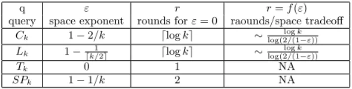
q ε r r=f(ε) query space exponent rounds forε= 0 raounds/space tradeoff

Ck 1−2/k dlogke ∼log(2log/(1k−ε)) Lk 1−dk/12e dlogke ∼

logk

log(2/(1−ε))

Tk 0 1 NA

SPk 1−1/k 2 NA

Table 2: The tradeoff between space and communication rounds for several queries.

atoms that join vertices at distance rad(q) fromvthat are not on any of the paths of length rad(q) fromv: these can be covered using paths of length rad(q) + 1 fromv.

As an application of this proposition, Table 2 shows the number of rounds required by different types of queries.

4.2 Lower Bounds for Multiple Rounds

Our lower bound results for multiple rounds are restricted in two ways: they apply only to an MPC model where com-munication at rounds ≥2 is of a restricted form, and they match the upper bounds only for a restricted class of queries.

4.2.1 Tuple-Based MPC

Recall thatMu1= (M 1 1u, . . . , M 1 `u), whereM 1 judenotes the

message sent during round 1 by the input server for Sj to the workeru. LetI be the input database instance, andq

be the query we want to compute. Ajoin tupleis any tuple inq0(I), whereq0 is any connected subquery ofq.

Thetuple-basedMPC(ε) model imposes the following two restrictions during roundsr≥2, for every workeru: (a) the message Muvr sent to v is a set of join tuples, and (b) for

every join tuple t, the workerudecides whether to include

t in Mr

uv based only on t, u, v, r and Mju1 , for all j s.t. t

contains a base tuple inSj.

The restricted model still allows unrestricted communica-tion during the first round; the informacommunica-tionM1

ureceived by

serveruin the first round is available throughout the com-putation. However, during the following rounds, server u

can only send messages consisting of join tuples, and, more-over, the destination of these join tuples can depend only on the tuple itself and onMu1. Since a join tuple is represented

using Θ(logn) bits, each server receivesO(n/p1−ε) join tu-ples at each round. We now describe the lower bound for multiple rounds in the tuple-based MPC model.

4.2.2 A Lower Bound

We give here a general lower bound for connected, con-junctive queries, and show how to apply it toLk, to tree-like queries, and to Ck; these results prove Theorem 1.2. We postpone the proof to the next subsection.

Definition 4.4. Letqbe a connected, conjunctive query. A setM ⊆atoms(q)isε-good forqif it satisfies:

1. Every subquery ofqthat is inΓ1ε contains at most one atom inM. (Γ1ε defined in Sec. 4.2.1)

2. χ(M) = 0, where M = atoms(q)−M. (Hence by Lemma 2.1,χ(q/M) =χ(q). This condition is equiva-lent to each connected component ofM being tree-like.)

An (ε, r)-plan M is a sequence M1, . . . , Mr, with M0 =

atoms(q)⊃M1 ⊃ · · ·Mr such that (a) for all j∈[r],Mj+1

is ε-good for q/Mj where Mj = atoms(q)−Mj, and (b) q/Mr ∈/Γ1ε.

(10)

Theorem 4.5. Ifqhas a (ε, r)-plan then every random-ized algorithm running in r+ 1 rounds on the tuple-based MPC(ε) model with p=ω(1)processors fails to compute q with probabilityΩ(nχ(q)).

We prove the theorem in the next section. Here, we show how to apply it to three cases. Assumep=ω(1), and recall thatkε= 2b1/(1−ε)c(Example 4.2). First, considerLk.

Lemma 4.6. Any tuple-based MPC(ε) algorithm that com-putesLk needs at leastdlogk/logkεerounds.

Proof. We show inductively how to produce an (ε, r

)-plan for Lk with r = dlogk/logkεe −1. The subqueries that are in Γ1ε are preciselyLk0 fork0≤kε, hence any set of

atomsMthat consists of everykε-th atom inL`isε-good for

L`for any`≥kε. LetM1be such a set starting with the first

atom. ThenLk/M1is isomorphic toLdk/k_εe. Forj= 2, .., r,

chooseMjto consist of everykε-th atom starting at the first atom inLk/Mj−1. Finally,Lk/Mj−1 will be isomorphic to

a path query of lengthL`for some `≥kε+ 1 and hence is not in Γ1. Thus M1, . . . , Mr is the desired (ε, r)-plan and

the lower bound follows from Theorem 4.5.

Combined with Example 4.2, it implies thatLk requires preciselydlogk/logkεerounds on the tuple-based MPC(ε). Second, we give a lower bound for tree-like queries, and for that we use a simple observation:

Proposition 4.7. Ifq is a tree-like query, andq0 is any connected subquery ofq,q0 needs at least as many rounds as qin the tuple-based MPC(ε) model.

Proof. Given any tuple-based MPC(ε) algorithmA for computingqinrrounds we construct a tuple-based MPC(ε) algorithmA0that computesq0inrrounds. A0will interpret each instance overq0 as part of an instance for q by using the relations inq0and using the identity permutation (Sj=

{(1,1, . . .),(2,2, . . .), . . .}) for each relation inq\q0. Then,

A0 runs exactly asAforr rounds; after the final round,A0

projects out for every tuple all the variables not inq0. The correctness ofA0follows from the fact thatqis tree-like.

Define diam(q), the diameter of a query q, to be the longest distance between any two nodes in the hypergraph ofq. In general, rad(q)≤diam(q)≤2 rad(q). For example, rad(Lk) =bk/2c, diam(Lk) =kand rad(Ck) = diam(Ck) =

bk/2c. Lemma 4.6 and Proposition 4.7 imply:

Corollary 4.8. Any tuple-based MPC(ε) algorithm that computes a tree-like queryq needs at leastdlogkε(diam(q))e rounds.

Let us compare the lower boundrlow =dlogkε(diam(q))e

and the upper boundrup=dlogkε(rad(q))e+1 (Lemma 4.3):

diam(q) ≤ 2rad(q) implies rlow ≤ rup, while rad(q) ≤

diam(q) impliesrup≤rlow+ 1. The gap between the lower

bound and the upper bound is at most 1, proving Theo-rem 1.2. Whenε <1/2, these bounds are matching, since

kε= 2 and 2rad(q)−1≤diam(q) for tree-like queries. The tradeoff between the space exponentε and the number of roundsrfor tree-like queries isr·log 2

1−ε ≈log(rad(q)).

Third, we study one instance of a non tree-like query:

Lemma 4.9. Any tuple-based MPC(ε) algorithm that com-putesCkneeds at leastdlog(k/(mε+ 1))/logkεe+ 1rounds, wheremε=b2/(1−ε)c.

Proof. Observe that any set M of atoms that are (at

least)kεapart along any cycleC`is-good forC`andC`/M

is isomorphic to Cb`/kεc. If k ≥ k r

ε(mε+ 1), we can

re-peatedly choose suchε-good sets to construct an (ε, r)-plan

M1, . . . , Mrsuch that the final contracted queryCk/Mr

con-tains a cycleC`0 with`0≥mε+ 1 (and therefore cannot be computed in 1 round by any MPC(ε) algorithm). The result now follows from Theorem 4.5.

Here, too, we have a gap of 1 between this lower bound and the upper bound in Lemma 4.3. ConsiderC5andε= 0;

rad(C5) = diam(C5) = 2,kε=mε= 2. The lower bound is blog 5/3c+ 1 = 2 rounds, the upper bound isdlog 3e+ 1 = 3 round. The exact number of rounds forC5is open.

As a final application, we show how to apply Lemma 4.6 to show that transitive closure requires many rounds (the proof is included in the full version of the paper).

Corollary 4.10. For any fixed ε < 1, there is no p -server algorithm in the tuple-based MPC(ε) model that uses o(logp) rounds and computes the transitive closure of an arbitrary input graph.

4.2.3 Proof of Theorem 4.5

Given an (ε, r)-planM(Definition 4.4) for a queryq, de-fineτ∗(M) to be the minimum ofτ∗(q/Mr), and the

mini-mum ofτ∗(q0), whereq0ranges over all connected subqueries ofq/Mj−1,j∈[r], such thatq06∈Γ1ε. Since everyq0satisfies τ∗(q0)(1−ε)>1 (byq06∈Γ1ε), andτ∗(q/Mr)(1−ε)>1 (by

the definition of goodness), we haveτ∗(M)(1−ε)>1.

Theorem 4.11. If q has an (ε, r)-plan Mthen any de-terministic tuple-based MPC(ε) algorithm running inr+ 1

rounds reports O(E(|q(I)|)/pτ∗(M)(1−ε)−1) correct answers in expectation over uniformly chosen matching databaseI.

The argument in Corollary 3.5 extends immediately to this case, implying that every randomized tuple-based MPC(ε) algorithm withp=ω(1) andr+1 rounds will fail to compute

qwith probability Ω(nγ(q)_{). This proves Theorem 4.5.}

The rest of this section gives the proof of this theorem. The intuition is this. Consider a ε-good setM; then any matching database i consists of two parts, i = (iM, iM),

whereiM are the relations for atoms inM, andi_M are the other relations. We show that, for a fixed instancei_M, the al-gorithmAcan be used to computeq/M(iM) inr+1 rounds; however, the first round is almost useless, because the algo-rithm can discover only a tiny number of join tuples with two or more atoms Sj ∈ M, since every subquery q0 of q

that has twoM-atoms is not in Γ1ε. This shows that the

al-gorithm computesq/M(iM) in onlyrrounds, and we repeat the argument until a one-round algorithm remains.

First, we need some notation. For a connected subqueryq0

ofq,q0(I) denotes as usual the answer toq0 on an instance

I. Whenever atoms(q0) ⊆ atoms(q00), then we say that a tuplet00∈q00(I) containsa tuple t0∈q0(I), ift0 is equal to the projection oft00on the variables ofq0; ifA⊆q00(I), B⊆

q0(I), thenAnB, called thesemijoin, denotes the subset of tuplest00∈Athat contain some tuplet0∈B.

Let A be a deterministic algorithm with r+ 1 rounds,

k∈[r+ 1] a round number,ua server, andq0 a subquery of

q. For a matching database inputi, definemA,u,k(i) to be the vector of messages received by serveruduring the first

krounds of the execution ofAon inputi. DefinemA,k(i) = (m1, . . . , mp), wheremu=mA,u,k(i) for allu∈[p], and:

(11)

KmA,u,k(q 0

) ={t0∈[n]vars(q0)| for all matching databasesi, mA,u,k(i) =m⇒t0∈q0(i)} KmA,k(q 0 ) =S uK A,u,k mu (q 0 ) A(i) =K_mA,r+1 A,r+1(i)(q). K_mA,u,k A,u,k(i)(q 0 ) andK_mA,k A,k(i)(q 0

) denote the set of join tuples fromq0 known at roundk by server u, and by all servers, respectively, on inputi. A(i) is w.l.o.g. the final answer of

Aon inputi. Define JA,q(i) =S {KA,_m1 A,1(i)(q 0 )|q0 connected subquery ofq} JεA,q(i) =S{KmA,A,11(i)(q 0 )|q0∈/Γ1ε connected subquery ofq} JεA,q(i) is precisely the set of join tuples known after the

first round, but which correspond to subqueries that are themselves not computable in one round; thus, the number of tuples inJεA,q(i) will be small. Next, we need two lemmas.

Lemma 4.12. Letq be a query, andM be anyε-good set forq. IfAis an algorithm withr+ 1rounds forq, then for any matching databasei_M over the atoms ofM, there exists an algorithmA0 withrrounds forq/M such that, for every matching databaseiM defined over the atoms ofM:

|A(iM, i_M)| ≤ |q(iM, i_M)nJεA,q(iM, iM)|+|A 0

(iM)|.

In other words, the algorithm returns no more answers than the (very few) tuples inJ, plus what another algorithm

A0 (to be defined) computes forq/M inone lessrounds.

Proof. The proof requires two constructions.

1. Contraction. Callq/M the contractedquery. While the original queryq takes as input the complete database

i= (iM, iM), the input to the contracted query is onlyiM.

We show how to use the algorithm A for q to derive an algorithm, denotedAM, forq/M.

For each connected component C of M, choose a repre-sentative variable zc ∈ vars(C); also denote SC the result of applying the queryC toi_M; Sc is a matching, because

C is tree-like. Denote ¯σ = {σx | x∈vars(q)}, where, for every variablex∈vars(q),σx is the following permutation on [n]: if x 6∈ vars(M) then σx = the identity; otherwise

σx = Πxzc(SC), for the unique connected component s.t. x ∈ vars(C). We think of ¯σ as permuting the domain of each attribute x ∈ vars(q). Then ¯σ(q(i)) = q(¯σ(i)), and ¯

σ(i_M) = id_M the identity matching database (where each relation inM is{(1,1, . . .),(2,2, . . .), . . .}), and therefore:

q/M(iM) =¯σ−1(Π_vars(_q/M₎(q(¯σ(iM),id_M))) (We assume vars(q/M) ⊆ vars(q); for that, when we con-tract a set of nodes of the hypergraph, we replace them with one of the nodes in the set.)

The algorithmAM forq/M(iM) is this. First, each input server forSj∈M replacesSjwith ¯σ(Sj) (sincei_M is fixed, it is known to all servers, hence, so is ¯σ); next, runA un-changed, substituting all relationsSj∈M with the identity; finally, apply ¯σ−1to the answers and return them. We have:

AM(iM) = ¯σ−1(Π_vars(_q/M₎(A(¯σ(iM),id_M))) (9)

2. Retraction. Next, we transformAM into a new algo-rithmRA_M called theretractionofAM, as follows:

(a) During round 1 ofRA_M, each input server forSjsends (in addition to the messages sent byAM) every tuple int∈

Sjto all serversuthat eventually receivet. In other words, the input server sends t to every u for which there exists

k∈[r+ 1] such thatt∈KAM,u,k

m_{AM ,u,k}(IM)(Sj). This is possible

because of the restrictions in the tuple-based MPC(ε) model: all destinations of t depend only on Sj, and hence can be computed by the input server. Note that this may increase the total number of bits received in the first round by a factor ofr, which isO(1) in our setting. RA_M will not send any atomic tuples during roundsk≥2. (b) In round 2,RAM

sends notuples. (c) In roundsk≥3,RA_M sends a tuplet

from uto vif server uknowst at roundk, and algorithm

AM sendstfromutovat roundk.

It follows that, for each roundk, and for each subqueryq0

ofq/Mwith at least two atoms,K_mRAM₍_i₎ ,u,k(q0)⊆KAM,u,k m(i) (q

0

): in other words,RA_M knows a subset of the non-atomic tu-ples known by AM. Moreover, let JAM

+ (iM) be the set of

non-atomic tuples known byAM after round 1,JAM

+ (iM) =

S

{K_mRAM₍_i₎ ,u,1(q0)|q0 has at least two atoms}: these are the tuples that we refused to sent in round 2. Then:

AM(iM)⊆(q/M(iM)nJ+AM)∪RAM(iM) (10)

SinceRAMwastes one round, we can compress it to an

al-gorithmA0with onlyrrounds. To prove the lemma, we con-vert (10) into a statement aboutA. (9) already showed that

AM(iM) is related toA(iM, iM). Now we show howJ AM + is related toJA,q ε (i): J AM + (iM)⊆σ −1_(Π vars(q/M)(J A,q ε (¯σ(i))))

because, by the definition ofε-goodness, if a subqueryq0 of

qhas two atoms inM, thenq06∈Γ1

ε. (10) becomes: AM(iM)⊆(q/M(iM)nΠvars(q/M)(J A,q ε (i)))∪¯σ −1 (A0(iM)) The lemma follows fromq/M(iM)nΠvars(q/M)(J

A,q ε (i))⊆

Π_vars(_q/M₎(q(i)nJεA,q(i)) and |AM(iM)|=|A(iM, iM)|, by

(9).

Lemma 4.13. Letq be a conjunctive query, andq0 a sub-query; if i is a database instance for q, we write i0 for its restriction to the relations occurring inq0. LetB be any al-gorithm forq0(meaning that, for every matching databasei0, B(i0)⊆q0(i0)), and assume that E[|B(I0)|]≤γ·E[|q0(I0)|]. Then, E[|q(I)nB(I0)|]≤γE[|q(I)|]whereI is a uniformly

chosen matching database.

While, in general,q0may return many more answers thanq, the lemma says that, ifBreturns only a fraction ofq0, then

qnBreturns only the same fraction ofq.

Proof. Let ¯y= (y1, . . . , yk) be the variables occurring in

q0. For any ¯a∈[n]k_{, let}_σ

¯

y=¯a(q(i)) denote the subset of

tu-plest∈q(i) whose projection on ¯yequals ¯a. By symmetry, the quantityE[|σy¯=¯a(q(I))|] is independent of ¯a, and

there-fore equalsE[|q(I)|]/nk_{. Notice that}_σ

¯ y=¯a(B(i0)) is either∅ or{¯a}. We have: E[|q(I)nB(I0)|] =P¯a∈[n]kE[|σy¯=¯a(q(I))nσy¯=¯a(B(I0))|] =P ¯ a∈[n]kE[|σ¯y=¯a(q(I))|]·P(¯a∈B(I0)) =E[|q(I)|]·P ¯ a∈[n]kP(¯a∈B(I 0 ))/nk₌_E[_|_q₍_I₎_|_]_·_E[_|_B₍_I0 )|]/nk

Repeating the same calculations forq0 instead ofB, E[|q(I)nq0(I0)|] =E[|q(I)|]E[|q0(I0)|]/nk

The lemma follows immediately, by using the fact that, by definition,q(i)nq0(i0) =q(i).