Anomaly Detection and Fault Localization Using Runtime State Models

(1)

Anomaly Detection and Fault

Localization Using Runtime State

Models

by

Xi Cheng

A thesis

presented to the University of Waterloo in fulfillment of the

thesis requirement for the degree of Master of Applied Science

in

Electrical and Computer Engineering

Waterloo, Ontario, Canada, 2016

c

(2)

I hereby declare that I am the sole author of this thesis. This is a true copy of the thesis, including any required final revisions, as accepted by my examiners.

(3)

Abstract

Software systems are impacting every aspect of our daily lives, making software failures expensive, even life endangering. Despite rigorous testing, software bugs inevitably exist, especially in complex systems. Existing tools to aid debugging, such as tracing, profiling, and logging facilities, reveal the behavior of a program’s execution; however, they require the developers to manually correlate the data to diagnose faults.

This work is the first to introduce the Runtime State Model, a summarization of a program’s behavior, for software anomaly detection and fault localization. A Runtime State Model is constructed from variables’ value change events of an execution. It consists of a set of states, and state transitions, where a state is a set of variables with their current values, and a state transition is induced by a variable’s value change. Comparisons between states from difference executions can be conducted to detect software anomalies. Deviations from the healthy states also help explain and locate faults in the source code. To automate this process, we implement Xtract, a facility that automatically extracts runtime traces from the Java Virtual Machines and constructs Runtime State Models for multiple simultaneous Java applications. Our evaluation provides evidence that Runtime State Models might be effective in detecting and locating injected faults to a RUBiS server with Xtract.

(4)

Acknowledgements

I would like to take this opportunity to express my appreciation to my supervisor Paul A. S. Ward for introducing me to the world of research and for his guidance and support throughout my Master’s degree program. I am grateful to Bernard Wong and Lin Tan for being my thesis readers, whose constructive comments and feedback helped improve the work.

This thesis is made possible with valuable assistance from many individuals since the beginning of the project. I thank the members of the Shoshin Lab for sharing their thoughts and providing insightful discussions. My appreciation also goes to the staff of the CSCF and the Department of ECE for their technical and administrative assistance.

To my lovely friends and those who had been part of my life, thanks for your inspi-rations, enthusiasm, friendship and love. This journey would not have been as enjoyable without all the fun and laughter we had, through ups and downs.

My deepest gratitude goes to my mom, Xiaozhen Wang, for her selfless love, uncondi-tional support and encouragement along the way.

(5)

Dedication

(6)

List of Tables

2.1 A Summary of Common RDD Operations . . . 16

2.2 A Summary of GraphX Operators . . . 18

6.1 A Summary of RUBiS Operations . . . 58

6.2 An Evaluation of the Performance Overhead of Xtract . . . 60

6.3 Anomaly Inducing Variables of the nulldb Case . . . 64

6.4 Anomaly Inducing Variables of the dbdown Case . . . 66

(11)

List of Figures

2.1 A Simple Function Generating 3 Change Events . . . 8

2.2 An example of the Mapping between Java Bytecodes and Local Variables . 12 2.3 An Example of Network Word Counting with Spark Streaming . . . 16

4.1 Xtract RPC Service Structure . . . 26

4.2 A Comparison of Regular to Asynchronous and Streaming RPCs . . . 28

4.3 An Example of GetClassMethods . . . 31

4.4 Sequence Diagram of the Xtract RPC Service, an Example . . . 32

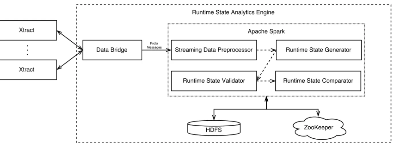
5.1 System Structure of the Runtime State Analytics Engine . . . 39

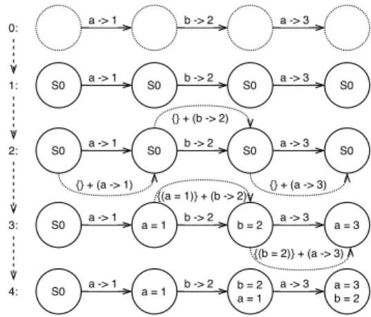
5.2 An Example of State Machine Construction . . . 44

5.3 Building State Machines with GraphX . . . 45

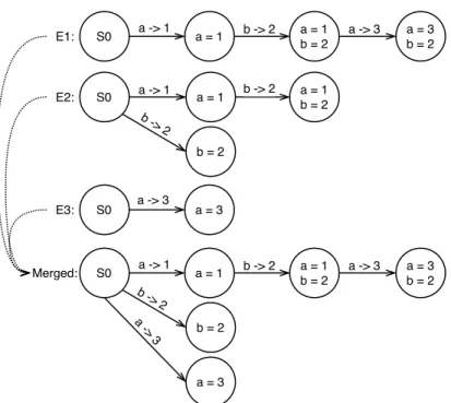
5.4 An Example of Incorrect Merging of State Machines . . . 48

5.5 An Example of Merging State Machines with the Cumulative Sliding Win-dow Approach . . . 50

5.6 An Example of State Machine Pruning . . . 51

6.1 Experiment Setup . . . 56

6.2 Faults Injected to the RUBiS Server . . . 63

6.3 Anomaly Detection of the nulldb Case . . . 65

6.4 Anomaly Detection of the conf Case . . . 67

(12)

A.2 A List of Core Interfaces of Xtract . . . 80

B.1 Custom Kryo Serializer for Protocol Buffer Messages in Spark 1.6 . . . 83

(13)

Chapter 1 Introduction and Motivations

With the popularity of computers, mobile devices and easier access to the Internet, software systems are impacting every aspect of our daily lives, making software failures expensive, even life endangering. Despite rigorous testing in almost all production software, software bugs still inevitably exist, especially in the complex systems. Take Boeing’s newest 787 Dreamliner as an example: it was discovered, after nearly 4 years in service, that an integer overflow bug in its generator control unit would cause a complete electric shutdown and potentially loss of control of the aircraft [29].

For enterprise entities, software failures result in capital losses. In August 2012, Knight Capital Group lost $440 million in 45 minutes due to a software failure, causing its stock price to drop by nearly 60% in one day [54].

A survey conducted from October to November 2014 reveals that [22],

• the average cost of unplanned application downtime per year is $1.25 billion to $2.5 billion for Fortune 1000 companies.

• the average hourly cost of an infrastructure failure is $100,000.

• the average cost of critical application failures per hour is $500,000 to $1 million.

Unfortunately, implementing reliable software has never been easy, even for the giants. On September 20, 2015, Amazon’s web services (AWS) experienced a 5-hour long outage, causing service interruptions for many of its big customers, including Netflix, Airbnb, IMDb, and Amazon’s own online markets [17], despite of its commitment to provide a minimum of 99.95% monthly uptime in the Service Level Agreement [32].

(14)

Approaches to improve software dependability has been extensively explored, by both Systems and Software Engineering communities. As a couple of representatives, replica-tion techniques create and coordinate replicas to increase system availability [1, 12, 37], rollback recoveries restore the failing processes to a state before the presence of failures [13,34,35], crash only software is designed that its components could be restarted without prior synchronizations [8, 9, 45], software rejuvenation prevents the occurrence of failures by proactively cleaning up the system’s internal states [26,31]. These approaches are step-ping stones towards today’s dependable services. They reduce the end-to-end visibility of failures, improving the MTTF (Mean Time To Failure) by orders of magnitude, however, will not help in fault diagnosis, i.e., debugging.

Runtime tracing is the most intuitive approach when it comes to debugging. The basic form of runtime tracing that most are familiar with is to use a debugger, e.g., gdb, to step over each line of the source code while inspecting variable values to find the bug. In this case, debugging is a process of inspecting a program’s execution paths and variable changes, i.e., states, that deviate from a developer’s expectations.

Efforts to ease this process focus on providing mechanisms to reveal the inner workings of a program through static instrumentations [30], dynamic instrumentations [11], or OS events tracking [2, 7]. In the context of a networked system, approaches also consider request flows between components [24,51]. Runtime tracing is often perceived as a mature technique extensively used even in production systems [11,51], however, these approaches merely provide means to retrieve runtime data and expect the developers to manually correlate the data to diagnose faults.

The automation of diagnosing program faults and anomalies is usually achieved through behavior matching, where the behavior of a program is defined as observable effects in its execution [5]. Early work towards automated fault detection takes descriptions of programs’ expected behaviors as input [5,47, 49], and therefore requires great efforts from the developers to manually define their expectations.

This limitation is addressed by the automated construction of program behavioral mod-els. It is observed that program behavioral models presented in existing work fall generally into two categories,

• In the context of performance diagnosis, models are constructed from performance costs, including, system resource consumptions [4], the running time of system calls [3], time spent on network requests [50] or information recorded in the log messages [44, 60], e.g., timing, number of records. However, these models can not be applied to the diagnosis of non-performance related issues.

(15)

• To detect more generic types of faults, flows and paths are usually used to model a system’s behavior. For the case of diagnosing componentized systems, request flows and status are adopted in anomaly detection [10, 14], but they are implementation-agnostic, and can only be used to determine the failing components. Attempts to model execution paths suffer from high false positives [27].

To address these limitations and achieve the automated detection of generic faults, at a source code granularity, we propose the use ofRuntime State Models in anomaly detection and fault localization. To define aRuntime State Model, we first refer to Lamport’s defini-tion of a computation, that a computation is a sequence of steps that result in transitions ofstates [36].

In the context of software, the following observations are made,

• a state is represented by a set of (variable, value) pairs,

• a step, i.e., a transition of states, is induced by the change of a variable’s value,

• and therefore, a sequence of variable’s value changes defines a program’s behavior.

This leads to one of the fundamental arguments of the work, that

Argument: Given that a runtime trace, i.e., sequence of variable’s value changes, defines the program’s behavior, a model constructed from a runtime trace to include a set of its states, and a set of state transitions, summarizes the behavior of an execution. We define the model as a Runtime State Model.

Note that a runtime trace captures the temporal order between the changes; however, the set of transitions in a Runtime State Model ignores their temporal property. It is also worth noting that to preserve the compactness of a Runtime State Model, each state in the model could be a subset of the program’s corresponding states to exclude outliers. To summarize the common behavior of a program, a model can be constructed from multiple runtime traces of the same program to include the shared states and transitions.

Intuitively, aRuntime State Model gradually constructed from a healthy execution, or a collection of healthy executions (of the same program), consists of healthy states that summarize the program’s healthy behavior. By comparing the states of a failing execution to the healthy states, we could derive a set of anomalous states, i.e., states that deviate from the healthy states, and a set of transitions that eventually lead to the anomalous

(16)

states. Since each state transition is a variable’s value change, it helps us locate the fault back to the source code.

The advantages of using Runtime State Models in anomaly detection and fault local-ization include,

• Anomalies detected with a Runtime State Model could be mapped back to the source code, achieving fault localization at a source code granularity.

• As opposed to models constructed from particular metrics, aRuntime State Model is constructed directly from runtime traces, which makes it capable of detecting generic faults.

• Constructing aRuntime State Model is an application-agnostic process and does not require knowledge of the system structure or source code beforehand, which also makes this technique applicable to all types of applications.

To the best of our knowledge, we are the first to formulate the notion ofRuntime State Models in the context of anomaly detection and fault localization. This work focuses on the automated construction ofRuntime State Models, and showing evidence that Runtime State Models might be effective in detecting runtime anomalies.

We recognize the following novel and significant contributions,

1.1 Contributions

• This work is the first to formulate the notion of using Runtime State Models in the context of software anomaly detection and fault localization.

• We presentXtract, a facility that automatically extracts runtime traces from the Java Virtual Machines and constructs Runtime State Models for multiple simultaneous Java applications. The facility includes,

– ARuntime Data Extraction Infrastructure that retrieves runtime traces directly from the Java Virtual Machines through a set of JVMTI constructs. As an effort to extract local variable change events from the JVMs, we implement the local variable watchpoint functionality through runtime breakpoints.

(17)

– A scalable and massively parallel Runtime State Analytics Engine on Apache Spark that achieves the construction and validation of Runtime State Models from multiple simultaneous input sources, through efficient graph analytics. The engine supports the online construction of Runtime State Models on streams of runtime events captured throughout the course of programs’ executions.

• First to evaluate the effectiveness of using Runtime State Models in the context of software anomaly detection. We introduce three types of injected faults to the RUBiS server, and show evidence that the Runtime State Models could help detect runtime anomalies and provide useful information in fault localization.

1.2 Thesis Outline

This thesis is consisted of 7 chapters.

• InChapter 2, we provide background knowledge that are relevent to the understand-ing of this thesis, includunderstand-ing the formal definitions of Runtime States and Runtime State Transitions and Runtime State Models, along with brief introductions to the technologies used in the implementation of Xtract.

• In Chapter 3, we discuss related work that approached the problem of software fault and anomaly detection, with runtime traces, log messages, and system metrics.

• In Chapter 4, we present the design and implementation of our Runtime Data Ex-traction Infrastructure that works to extract the runtime information of applications directly from the Java Virtual Machines.

• InChapter 5, we present the design and implementation of our scalable and massive parallel Runtime State Analytics Engine. We also describe a set of graph algorithms used by the engine to construct, validate and compare the Runtime State Models.

• In Chapter 6, we talk about our experiment setup and environment; discuss ex-periments conducted to evaluate the performance overhead of Xtract, and show how Runtime State Models help us in detecting and locating faults injected to a RUBiS server.

• We conclude in Chapter 7, identify, and list issues in current state of the work as future work.

(18)

Chapter 2 Background

In this chapter, we formalize the definitions of Runtime States, Runtime State Transi-tions, and Runtime State Models used throughout this thesis. We also provide necessary background information that are relevant to the understanding of our approaches, and technologies used extensively in our implementations.

2.1 Terminologies and Definitions

To formalize the definition of a Runtime State Model, we first refer to Lamport’s formal definition of acomputation [36,38],

Lamport’s Definition of a Computation: A computation is a sequence of steps,

< s, α, t >, where s and t are states and α is an action. A behavior is a sequence

s1 α1 −→s2 α2 −→s3 α3

−→ . . .. The step < si, αi, si+1 > represents a transition from state si to state si+1 that is performed by action αi.

In the context of this thesis, we define a state as a set of (variable, value) pairs, a step as a transition of states induced by the change of a variable’s value, and use a sequence of variable’s value changes to define a behavior.

2.1.1 Runtime Trace

(19)

Definition: ARuntime TraceRT is asequence e1, e2, . . . from contiguous

observa-tions o1, o2, . . ., where each ei ∈ RT indicates a variable’s value change event. Each change event e = (v → valv) represents the value of variable v has been changed to

valv.

2.1.2 Runtime States and Transitions

Runtime States and Runtime State Transitions are derived from a Runtime Trace. We derive our own formal definitions of Runtime States, and State Transitions, based on Lamport’s definition of acomputation, as follows,

Definition: A Runtime State si is a set of variables with values, derived from a Runtime Trace RT = e1, . . . , ei, in their temporal order. Each variable (v = valv) represents the variable v has a most recent value of valv. A Runtime State without any variables is defined as the initial state s0.

One state is transitioned to another state through a state transition, where

Definition: ARuntime State Transitiontsrc→dst= (ssrc, sdst, e) represents a tran-sition from state ssrc to state sdst, given a variable value change evente.

2.1.3 Runtime State Models

A Runtime State Model is aset of Runtime Statesand aset ofRuntime State Transitions. We give the formalized definition of aRuntime State Model as follows,

Definition: Given a set of Runtime States S = s0, s1, . . . sn, and a set of Runtime State Transitions T = {ti→j|si, sj ∈ S, i 6= j}. A Runtime State Model, G = (S0, T0), is a set of Runtime States S0 = s0₀, s0₁, . . . s0_n, where s0_i ⊆ si, and a set of Runtime State Transitions T0 ={t0_i_→_j|s0_i, s0_j ∈S0, i6=j}.

EachRuntime State in the model is reachable from each other, if there exists aRuntime State Transition between the states. A Runtime State Model is represented with a state machine, a directed graph with each vertex being aRuntime State, and each edge being a Runtime State Transition.

(20)

1 i n t s i m p l e f u n c t i o n ( ) {

2 i n t a = 1 ; 3 i n t b = 2 ;

4 a = 3 ;

5 }

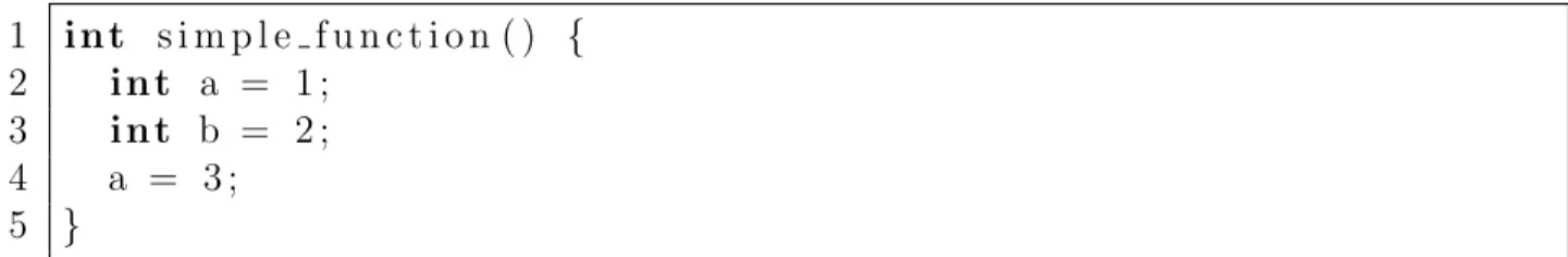
Figure 2.1: A Simple Function Generating 3 Change Events

2.1.4 Runtime State Pruning

Runtime State Pruning is the process of computing a set ofRuntime StatesS0, where each state s0 ∈ S0 is a subset of the original states s ∈ S derived from a Runtime Trace. We define the process of Runtime State Pruning as follows,

Definition: Given a set of variablesV =S

v,∀v ∈s,∀s∈S, whereS =s0, s1, . . . , sn is the originalset ofRuntime States. Derive a set of statesS0, whereS0 =s0₀, s0₁, . . . , s0_n,

s0_i ⊆si,∀i ∈[0, n], such that v0 ∈V0, ∀v0 ∈s0,∀s0 ∈ S0, whereV0 ⊆V. We define the process of deriving S0 as Runtime State Pruning.

2.1.5 Universal Runtime State Models

We define the common subgraph shared by multipleRuntime State Models as a Universal Runtime State Model. We formalize the definition of a Universal Runtime State Model as follows,

Definition:Given a set ofRuntime State Models,G1 = (S1, T1), G2 = (S2, T2), . . . , Gn = (Sn, Tn). A Universal Runtime State Model Gu = (Su, Tu) is such that s ∈ Su, iff, s ∈S1∩ · · · ∩Sn, ∀s∈S1∪ · · · ∪Sn, and Tu ={ti→j|si, sj ∈Su, i6=j}

Given that a Runtime State Model summarizes the behavior of a program, a Universal Runtime State Model summarizes the common behavior of a set of executions.

2.1.6 Case Study

Take the example in Figure2.1, at the time of observation, if the control is at source code line 3, we say the runtime state at observation oi is si = {(a = 1)} with a transition

(21)

ti−1→i = (si−1, si,(a → 1)). When the control reaches line 4, we say the runtime state at observation oi+1 is si+1 ={(a = 1),(b = 2)} with a transition ti→i+1 = (si, si+1,(b → 2)).

When the control reaches line 5, and updates the value of a, we say the runtime state at observation oi+2 is si+2 = {(a = 3),(b = 2)} with a transition ti+1→i+2 = (si+1, si+2,(a →

3)).

2.2 Java Virtual Machine Internals

This thesis focuses on the extraction and analysis of runtime information of Java applica-tions, and therefore, requires the knowledge of basic internals of the Java Virtual Machine. In this section, we discuss and explain some of the mechanisms essential to the understand-ing of the rest of the thesis, in a nutshell.

2.2.1 Java Methods, JIT, and Debugging Support

Before executing a Java application, one needs to first compile Java source files usingjavac, which compiles Java code into JVM bytecodes, stored in class files. When starting a Java application, JVM will first load all classes into the VM, this process parses the class files, and stores methods in a special space in the heap, containing information of method types, method bytecodes, local variable tables, etc. Each method is identified by a unique ID associated with its enclosing class.

One interesting question that many may have is how is JIT, Java’s Just in Time com-pilation going to impact the management of, and the subsequent interactions with Java methods. Java’s JIT compiler aims at improving the performance of Java applications by optimizing, and eventually replacing Java’s platform independent bytecodes to native machine instructions. Despite different JVM implementations, most adopt the hot code replacement strategy that only optimizes heavily used function through careful calculations due to the fact that the overhead of code compilation and replacement could be substantial [6].

Take Hotspot VM as an example, it offers both bytecode optimization and JIT compi-lation mechanisms that would progressively apply optimizations until eventually swapping bytecode to machine code [21]. While the replacement and compilation strategies are be-yond the scope of this thesis, we will discuss how this affects the debugging of a Java application as follows.

(22)

A JVM is capable of providing full debug support while maintaining as many enabled optimizations as possible. Setting breakpoints as an example, the JVM will insert a break-point opcode at the corresponding instruction locations of the original bytecodes, and each version of the optimized bytecodes if any. Given that a bytecode may be optimized dur-ing execution, whenever a breakpoint is reached, the virtual machine would preserve all Java states, and temporarily fall back to use the original bytecode for debugging purposes. Since it is impossible to debug native machine code through the JVM interpreter, setting a breakpoint would disable further JIT compilations on the method until all breakpoints on the method are cleared. If a method is already JIT compiled at the point a breakpoint is being set, the method will be deoptimized [20], i.e., the JVM will fall back to use bytecode interpretation for that method without compromising program states with OSR (On Stack Replacement).

2.2.2 Java Local Variables and Bytecodes

Each Java method has a list of local variables, the number and length of which are deter-mined and stored in the class files during compile time. A Java local variable typically has the following metadata, the notions of which will be used throughout the thesis,

• slot, the logical position of the variable in the list, used and identified by the virtual machine.

• start location, the index of bytecode instructions where the local variable is first available.

• length, the length of the valid section for the local variable, i.e., the last bytecode instruction that this local variable is valid is start location+length.

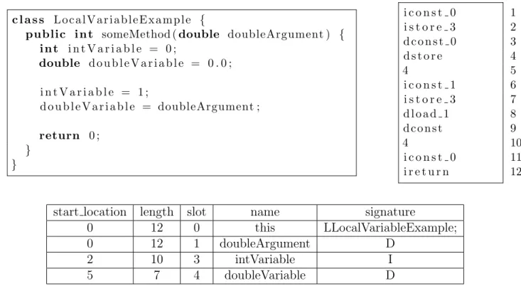
Java local variables could be either a Java primitive, or a reference to an object that is stored in the Java heap. Accesses and Modifications to a Java local variable are translated to bytecode instructions to load or store values to a specific local variable slot. An example showing the mapping between the Java bytecodes and Java code is depicted in Figure2.2, in which the upper left listing shows the original Java code that a method takes one argument, initializes and modifies two local variables. The Java code is compiled into a series of bytecodes as in the upper right listing that will be discussed later, and a list of local variables as shown in the table. Both bytecode instructions and the local variable table are extracted from the compiled class file usingjavap.

(23)

Although we will not go deep into Java bytecode instructions, we briefly discuss the instructions used here to explain how local variables are accessed by a Java program. There are three categories of instructions in the upper right list, where <t>const <i> pushes a constanti of typet into the operand stack, <t>store <i> stores a value of type t on the top of the operand stack back to the local variable at slot i, and <t>load <i> load the value of type t at slot i to the operand stack. Note that if the slot number i too large to be represented by a single instruction, two instructions will be used with the second instruction being the slot number, as in lines 4-5 and lines 9-10. That said, we can now walk through the bytecodes as follows,

The interpreter first pushes integer 0 into the stack, and stores it to local variable at slot 3, i.e.,intVariable, this corresponds to the Java code line 3. The same logic is followed by instructions 3-5 corresponding to Java code line 4, and instructions 6-7 corresponding to Java code line 6. For Java code line 7, one needs to first load the value ofdoubleArgument and store its value into variabledoubleVariable, this corresponds to instructions 8-10.

The local variable table has the information of each local variable per method, including their slot number, start location, length, variable name and signature. In our example, 4 local variables exist in someMethod. Note that, for a member method, slot 0 is always reserved for this object. Since all of the local variables in this case are reachable until the end of the method, the last instruction that the variables are valid is start location+

length = 12, though their start locations vary. Since both this and doubleArgument are reachable since the entry of the method, theirstart location are 0, while the start location ofintVariable and doubleVariable are 2 and 5 respectively.

2.3 JVM Tooling Interface

The JVM Tooling Interface (JVMTI) is a set of APIs provided by Java Virtual Machines to inspect the states and control the execution of Java applications [16].

To use the JVMTI interfaces, one needs to implement a client, namely agent. An agent is essentially a shared library written in C/C++, loaded by the JVM at startup time, and piggybacks on the JVM process. One could ask the JVM to load an agent by specifying the agent path and options inJAVA OPTS1.

The JVMTI provides control mechanisms that fall into various categories, however, we discuss only two of those that are used extensively in our implementation.

(24)

1 c l a s s L o c a l V a r i a b l e E x a m p l e {

2 public i n t someMethod (double doubleArgument ) {

3 i n t i n t V a r i a b l e = 0 ; 4 double d o u b l e V a r i a b l e = 0 . 0 ; 5 6 i n t V a r i a b l e = 1 ; 7 d o u b l e V a r i a b l e = doubleArgument ; 8 9 return 0 ; 10 } 11 } 1 i c o n s t 0 2 i s t o r e 3 3 d c o n s t 0 4 d s t o r e 5 4 6 i c o n s t 1 7 i s t o r e 3 8 d l o a d 1 9 d c o n s t 10 4 11 i c o n s t 0 12 i r e t u r n

start location length slot name signature

0 12 0 this LLocalVariableExample;

0 12 1 doubleArgument D

2 10 3 intVariable I

5 7 4 doubleVariable D

(25)

2.3.1 Classes and Fields

A JVMTI agent has the capability to extract class information from the JVM. The Get-LoadedClasses function returns all class objects from the JVM that have already been loaded. TheGetClassSignature function gives the Java class signature of each class object. Together, one could easily implement logic to get a subset of useful classes according to the class signatures. A Java class usually defines fields and methods.

One could get a list of fields given a class object with GetClassFields. Java fields are uniquely identified as jfieldIDs in JVMTI, and are valid until their enclosing classes are garbaged collected or modified. The names and signatures of Java class fields could be extracted with GetFieldName.

2.3.2 Methods, Bytecodes, Breakpoints and Local Variables

Similar to Java class fields, one could extract a list of methods given a class object with GetClassMethods. Java methods are identified with a unique ID of type jmethodID in JVMTI, with which one could get various information of the method, including the name, the signature, the modifier, etc. Among the miscellaneous stuff one could extract from the JVM, we discuss two important pieces to our implementation: the method bytecodes and local variables.

As mentioned in Section 2.2.1, the bytecodes and local variables of Java methods are generated and stored in the class files during compile time, and despite JVM’s optimizations to the bytecodes, it will always fall back to use the original bytecodes if in debug mode. That said, GetBytecodes function returns an array of original bytecodes as compiled by javac given ajmethodID, with each element being a single bytecode instruction.

One could set breakpoints at various bytecode locations usingSetBreakpoint that takes two parameters, the method id, and the index of the instruction in the array, at which to set the breakpoint. Setting breakpoints on a method immediately deoptimizes the method, and invalidates its capability to be JIT compiled until all breakpoints on the method are cleared. Events could be enabled on the breakpoints. If a breakpoint is reached, a breakpoint event will be triggered invoking a user-defined callback function. We discuss JVMTI events in Section 2.3.3

A mapping from bytecode locations back to the Java code locations could be obtained through GetLineNumberTable. One could also extract a list of local variables given a Java method. The GetLocalVariableTable function takes a method id, and returns a list of Java

(26)

local variables including theslot,start location,length, along with the name and signature of each variable defined in the method.

2.3.3 Event Management

JVMTI provides mechanisms to manage various JVM events, e.g., FieldModifications, FieldAccesses, Exceptions, Breakpoints, etc.

Event notifications are triggered by invoking corresponding event callback functions. A global struct containing callback function pointers of all event types are set at the agent loading phase through SetEventCallbacks. This also indicates that only one callback logic per event is permitted. Notifications could be enabled or disabled for each event with the function SetEventNotificationMode, globally or with a per thread granularity.

In the scope of this thesis, two events are of interests. The field modification event that is triggered whenever a field is modified, and the breakpoint event that is triggered whenever a breakpoint is reached.

To set a modification watchpoint on a Java class field, one needs to call SetFieldMod-ificationWatch providing the class object and the jfieldID of the field. If the watchpoint is no longer needed, ClearFieldModificationWatch could be called with the same set of arguments. A callback of the field modification event gives the following information,

• the thread that is modifying the field

• the method and instruction location that is modifying the field

• the class, signature, object of the field being modified

• the new value of the field

Similarly, to set a breakpoint, one need to call SetBreakpoint with thejmethodID and the location of instruction at which to set the breakpoint. Breakpoints could be cleared with ClearBreakpoints with the same set of arguments. The breakpoint event will be triggered before the execution of the instruction at which a breakpoint is set, and the callback of the breakpoint event gives information of the current thread, the method id and instruction location. The JVMTI and JNI environment pointers are provided in the breakpoint callback that could be used to access runtime information from the JVM. The thread will be temporarily suspended until the callback returns.

(27)

2.4 Apache Spark

Apache Spark is a batch processing system that claims to be up to 100x faster than Hadoop MapReduce in memory [53]. We use Spark extensively in our runtime data analysis and modelling process. In this section we briefly discuss various components of Spark that we adopt in our implementation.

2.4.1 Resilient Distributed Dataset (RDD)

Spark uses Resilient Distributed Dataset (RDD) to achieve fault-tolerant distributed in-memory batch processing [58].

An RDD is a read-only, partitioned collection of records. Unlike in Distributed Shared Memory (DSM) where processes are allowed to read and write to a particular address, RDDs only provide coarse grained transformations, i.e., map, filter, reduce, etc, that enable the tracking of how an RDD is derived from other RDDs, or from the file system by logging those transformations (lineage), which could be later used in system recoveries in the presence of failures. Other benefits of RDDs over DSM include the ease of migrating jobs from slow nodes, the capability of fine-grained scheduling based on data locality, etc., according to the original paper [58].

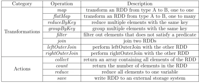
Operations on an RDD are divided into two categories, transformations and actions. A transformation is a lazy operation that define a new RDD, while an action launches a computation to calculate a value or write data to external storage. One RDD may be transformed multiple times before an action is applied. A summary of common RDD operations is shown in Table 2.1.

2.4.2 Spark Streaming and D-Streams

As an effort to support real-time streaming processing with Spark, discretized streams (D-Streams) is proposed to simulate real-time streaming with a batch processing framework [59].

A D-Stream groups input streams into a series of RDDs on small time intervals, and computes over the RDDs through batch processing. That said, one needs to first spec-ify a window size. Input data received in each window is stored across the cluster to form an input dataset, which is manipulated by users through RDD operations that act independently on each window.

(28)

Category Operation Description

Transformations

map transform an RDD from type A to B, one to one

flatMap transform an RDD from type A to B, one to many reduceByKey reduce multiple elements with the same key

groupByKey group multiple elements with the same key filter filter out elements that does not satisfy a predicate

join join two RDDs

leftOuterJoin perform leftOuterJoin with the other RDD rightOuterJoin perform rightOuterJoin with the other RDD

Actions

collect return an array containing all elements of the RDD count return the number of elements in the RDD reduce reduce all elements to one variable

save write RDD to an external storage system

Table 2.1: A Summary of Common RDD Operations 1 val s t r e a m i n g C o n t e x t = new S t r e a m i n g C o n t e x t ( . . . , S e c o n d s ( 1 0 ) ) 2 val l i n e s = s t r e a m i n g C o n t e x t . s o c k e t T e x t S t r e a m ( ” l o c a l h o s t ” , 7 0 0 0 ) 3 val words = l i n e s . f l a t M a p ( . s p l i t ( ” ” ) )

4 val wordCounts = word . map( x => ( x , 1 ) ) . reduceByKey ( + ) 5 wordCounts . p r i n t ( )

Figure 2.3: An Example of Network Word Counting with Spark Streaming

An example of counting the number of words in a network stream is shown in Figure

2.32. In the example, a window size of 10 seconds is specified on line 1. By creating a network text streaming from the localhost, Spark Streaming would create RDDs with records received in 10-second windows, and apply 2map and 1reduce operations on those RDDs, giving the count of words received in each window.

A D-Stream inherits all benefits of an RDD, including fault tolerance through RDD lineage. To achieve efficient recovery, an approach calledparallel recovery is introduced by periodically checkpointing some of the state RDDs, and asynchronously replicating them to other nodes. In the presence of a failure, multiple parallel tasks are launched to compute and recover different RDD partitions from the latest checkpoint.

2_{You can find the full code here:}

https://github.com/apache/spark/blob/master/examples/src/ main/scala/org/apache/spark/examples/streaming/NetworkWordCount.scala

(29)

2.4.3 Spark GraphX

Spark GraphX brings low-cost, fault-tolerant graph processing on a general-purpose data processing system, i.e., Apache Spark, that matches the performance of specialized graph processing systems [28]. Despite the great efforts made by Spark GraphX to optimize the representation, computation and partition of graph data, here we only discuss Spark GraphX from a user’s perspective, i.e., the operators Spark GraphX provides to facilitate graph computations.

Spark GraphX provides a graph abstraction, namely Graph[VD, ED], that has a

vertex type of VDand an edge type of ED. It takes two RDDs representing the vertices and edges of a graph respectively. Each vertex of a GraphX graph is a key-value pair of (VertexId, VD), while the VD could be any objects including user-defined structures. Each edge of a GraphX graph is in the form of a triple, (src VertexId, dst VertexId, ED), in which the first two elements indicate thesrc and dst vertex ids, and theED is an object describing the edge.

Spark GraphX supports both transformations on graph components, i.e., vertices and edges, as well as Pregel like operators. We provide a summary of GraphX operators in Table 2.2.

A Pregel-like operator implements a GAS message passing system with each vertex in the graph being an individual program [40]. In Spark GraphX, the Pregel implementation is implemented with batch processing operators that the user needs to provide four mandatory functions.

• vprog is used to simulate the vertex program that updates the state of each vertex according to incoming messages

• send message is used to generate messages to send to each of the neighboring vertices. If no messages are to be sent to a vertex, an empty message set could be generated. The entire process terminates when the number of active messages becomes 0.

• merge message is used to merge multiple messages into a single one before sending them out to a vertex. This is for performance considerations to reduce shuffling overhead.

• initial message is the initial message to be sent to all vertices before the first super step. An initial message could be empty.

(30)

Operator Description

mapTriplets transform the graph type from [VD, ED] to [VD, ED’] given each triplet mapVertices transform the graph type from [VD, ED] to [VD’, ED] given each vertex mapEdges transform the graph type from [VD, ED] to [VD, ED’] given each edge

subgraph filter out vertices and edges that does not satisfy predicates pregel run pregel like impl with user-defined vertex programs and messages

Table 2.2: A Summary of GraphX Operators

A triplet in the mapTriplets function is a notion provided by GraphX that describes a triple of (src vertex object, dst vertex object, edge). Different from an edge that only gives the ids of its src and dst vertices as provided, a triplet gives the actual objects of the three components.

We use Spark GraphX extensively in the building and analysis of software state ma-chines as part of our software state modeling process.

(31)

Chapter 3 Related Work

In the context of runtime anomaly detection, existing research generally falls into three categories:

1. approaches to detect runtime anomalies and locate faults through the analysis of runtime traces, where a runtime trace could be an execution path, or a request flow between networked components. These approaches normally require instrumenting the programs for data extraction,

2. anomaly detection through log mining makes use of the pervasive log messages most software systems produce to determine whether, how, and when a failure happens inside of the system,

3. and approaches to detect runtime anomalies through system metrics, i.e., CPU uti-lization, memory consumption, etc.

3.1 Runtime Tracing and Models

Runtime tracing is the most intuitive approach when it comes to debugging. Existing research is observed to focus on two different aspects of this problem. Research that focuses on runtime tracing techniques proposes tools and implementations to extract runtime data to reveal a program’s behavior. Efforts that focus on the automation of fault diagnosis using runtime traces usually construct models to look for behavior deviations. We discuss them separately

(32)

3.1.1 Runtime Tracing Techniques

Purify [30] uses static instrumentation to detect memory errors. It instruments C/C++ object files to add tracking code at each memory allocation and deallocation site. A memory error is reported if an address is accessed before allocation, or if an address is not properly deallocated.

As opposed to Purify, DTrace [11] uses dynamic instrumentations where each instru-mentation probe could be enabled or disabled. It is built in the system kernel to track function invocations, syscalls, locks, etc.

Anderson et al. propose continuous sampling on the OS level with performance coun-ters, and use an analysis tool to calculate time spent on each instruction, source code line, and procedure calls [2].

Bhatia et al. use fined-grained OS events, e.g., page allocations, process scheduling, block-level I/O, etc to detect system performance problems [7].

For the case of a networked system, approaches are proposed to track the request flows between distributed components.

X-Trace is a request tracing system for networked systems [24]. The idea is that each component of a networked system includes a metadata header in their message packets before sending them to the next hop, describing the identity of and operations conducted on the component. The system then analyzes the message flow and operation status of each component from a client on the receiving end to determine the failures of system components.

Dapper [51] is a production framework used inside of Google to trace RPC calls of a distributed system. It is a built into Google’s RPC framework that keeps track of the source, destination, operation and timing information of each RPC call, and presents them in a tree structure. The traces are stored in an external log file to be analyzed by other entities.

These approaches provide means to extract runtime data, but they expect the devel-opers to manually correlate the data to diagnose faults.

3.1.2 Expectations as a Model

Early efforts towards software fault diagnosis require manual input of expected program behaviors. These approaches usually employ special-purpose domain languages to describe an expectation.

(33)

Bates proposes the use ofEvent-Based Behavioral Abstraction, a model that uses events and attributes, e.g., for an open file event, the name and id of the file, to describe the behavior of a networked system.

Perl et al. use performance assertions to detect runtime performance anomalies. A developer needs to describe the expected performance metrics of various operations, e.g., I/O timing, lock wait time, cache hit rate, etc. Anomalies are reported if an operation fails the provided performance assertion [47].

Pip [49] is an infrastructure that detects unexpected behaviors in distributed systems. It requires programs to be linked against a library to generate events and resource mea-surements. It takes descriptions of the expected execution paths and performance metrics for each operation, and reports anomalies when mismatches are found.

3.1.3 Models from Performance Costs

Existing approaches that are designed to diagnose system performance issues usually con-struct cost models. Magpie [4] uses OS resource consumption events, e.g., bytes read, cache miss, etc., to establish a clustering model for each request.

Sambasivan et al. use request flows and the response time of each request captured by Dapper [51] to model the system performance in a directed weighted graph [50]. They use Kolmogorov-Smirnov test on response time and request counts to determine deviations in the request flows. The graph is used to identify anomalous flow ranked by the number of appearances.

X-ray [3] uses the execution paths and timing of each system call and synchronization operations to construct weighted directed graphs. The graph is then used to diagnose performance issues by looking at the edges with large weights.

These approaches focus on diagnosing system performance issues, and can not be ap-plied the diagnosis of non-performance related issues.

3.1.4 Models from Paths and Flows

Chen et al. designed Pinpoint, an instrumented J2EE middleware that tracks the client requests, internal and external failures [14]. This results in a matrix with each rowing being a single request, and each feature being the number of failures happened for each of the software components. A clustering algorithm is later applied on the generated matrix

(34)

to determine the failing component. However, it is implementation-agnostic, and can only be used to determine the failing components.

For efforts to detect more generic types of faults, Ghanbari et al. came up with a low-overhead real-time solution to detect runtime anomalies, namely, Stage-aware Anomaly Detection (SAAD) [27]. SAAD looks for software logging points, i.e., code statements that print out log messages, through source code analysis. They instrument the source code to, instead of printing out a message to a log file, send an event message to a remote analyzer. Further analysis are carried out through statistical testing, i.e., t-test on the execution flows and time spent in between consecutive logging points for the detection of flow and performance anomalies. This approach, however, suffers from high false positives.

We recognize ClearView [46] as the most related work to ours. ClearView is an au-tomatic error patching facility that corrects failing executions online by enforcing the ex-ecution paths. It constructs invariants, a model that captures the common control flows (a sequence of instructions and variable values) across multiple executions. Failures, for example, illegal control flow transfers and memory accesses, are detected by instrumented monitors. Whenever a failure is detected, ClearView repairs the actual execution by en-forcing the flow recorded in the invariant. This is in contrast to our goal of using invariant runtime states to detect anomalies and locate faults.

3.2 Log Mining

Log messages are pervasive, and are intended to be used to detect problems in any large-scale software. Analyzing runtime logs is usually an offline process, and therefore does not exert extra overhead on existing systems. Existing log analysis techniques usually take the following three approaches,

• Using natural language processing techniques that treat log messages as unstructured data.

• Inferring the structures of log messages through code analysis and annotations.

• Combining the efforts of machine learning techniques with manual data labeling.

In this section, we discuss approaches that use software logs to determine runtime anomalies.

(35)

Xu et al. use the console logs of a software system to detect anomalies [55]. Their approach requires the use of source code to recover the underlying structures of the log messages, and apply machine learning and information retrieval techniques to detect un-usual patterns in the logs.

SherLog [56] is a tool that infers information to help programmers understand what have happened during the failed execution. It uses both the software source code and the log messages to infer the execution path and variable values during the failed execution. They conclude thatSherLog is useful in diagnosing 8 real world software failures.

Nagaraj et al. present DISTALYZER, an automated tool to support developer investi-gation of performance issues in distributed system, by comparing the system logs to infer the variable values and event occurrences that exhibit the largest divergence across the log sets [44]. It compares the runtime logs by looking at bothevents, i.e., operations, and states, i.e., value of some system variables, and reports those information where perfor-mance variations are observed.

lprof [60], is a profiling tool that automatically reconstructs the execution flow of each request in a distributed application. It analyzes the application’s binary code and runtime logs to associate log messages with individual requests, i.e., identifying log messages on distributed nodes that belong to the same request, and shows diverging message patterns per request, thus helping developers to find bugs.

Despite the requirements of access to the source code of the above approaches, Reide-meister proposes treating log messages as unstructured text [48]. It clusters log message by tokenizing the log messages, and applying clustering based on the edit-distance between message tokens.

The effectiveness of log analysis approaches depends greatly on the quality of log mes-sages, i.e., counting on the developers to provide useful logging statements in the source code. Work that automatically inserts or enhances existing logging statements [57], requires instrumenting the source code.

3.3 System Metrics Models

Another relevant category of work uses system metrics data, i.e., CPU utilizations, mem-ory consumption, etc., to detect software anomalies. The use of system metrics achieves anomaly detection with complete ignorance of the implementations and structures of the software system under observation.

(36)

Jiang proposes the modeling of system metrics data with linear and information the-oretic models [33]. An unhealthy system state is determined through the fitness of the trained model given a data point representing the system state. System metrics can also be used to determine faulty components through the analysis of per-component metrics data.

Munawar et al. present approaches to discover system faults with linear correlations between system metrics data [41, 42, 43]. A correlation model relates multiple system metrics, and is sensitive to the fluctuations. Anormaly detection is achieved through the identification of mismatches between metric observations and predictions with the correlation models built with metrics of a health system.

These approaches can only be used to determine the failing components, but will not provide information to aid debugging.

(37)

Chapter 4 Runtime Data Extraction

Infrastructure

To construct runtime state models, and apply them in the context of software anomaly detection, we propose Xtract, a general-purpose facility that automatically retrieves run-time data from the Java Virtual Machines, and automates the process of constructing and analyzing runtime state models. We divide the facility into two components,

• A Runtime Data Extraction Infrastructure that retrieves runtime data directly from Java Virtual Machines, and exposes a set of APIs to the monitoring entity to control the types and granularities of data retrieved.

• A Runtime State Analytics Engine that constructs, validates and analyzes the run-time state models from simultaneous input sources.

We present theRuntime Data Extraction Infrastructure in this chapter.

The infrastructure, is designed to extract runtime information from the Java Virtual Machine. In addition to data extraction using JVMTI and JNI interfaces as described in Section2.3, it also implements logic to organize, serialize, and transport those data out of the Java Virtual Machine, and exposes a set of APIs to allow the external entity to control its behaviors.

We recognize two major component in the Xtract infrastructure.

• The Xtract RPC Service is a foundational service that provides efficient inter and intra components data serialization and transport support.

(38)

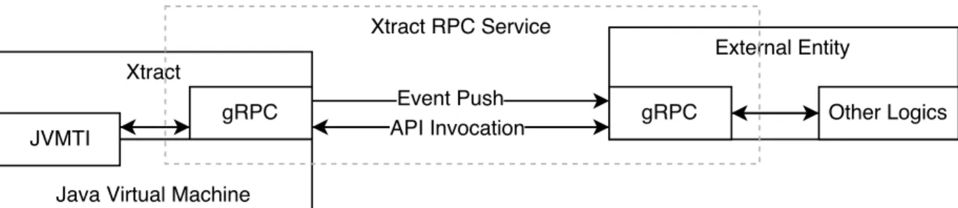
Figure 4.1: Xtract RPC Service Structure

• The Xtract JVMTI agent is a shared library that piggybacks on the Java Virtual Machine process. It exposes a set of higher level runtime inspection APIs to external entities through the RPC Service and makes use of the JVMTI and JNI interfaces to extract information from the JVM.

Our Runtime Data Extraction Infrastructure is implemented with 3,000 lines of C++ code for the JVMTI agent, 250 lines of Protocol Buffer definitions for the RPC service, and 300 lines of Go code. We describe each of the components separately as follows,

4.1 Xtract RPC Service

To accommodate communications between external entities and the infrastructure, a gRPC server is implemented in the shared library loaded by the JVM, and is initialized during the agent’s OnLoad phase, as depicted in Figure 4.1. The goals of the RPC service are three folds:

1. External entities are able to get data out of the Java Virtual Machine on demand by calling corresponding interfaces.

2. The external entity could configure Xtract on the fly through a set of control APIs, e.g., to enable or disable an event or toggle the watchpoints or breakpoints during runtime.

3. The RPC service decouples the JVMTI agent implementations and data analytics logics in the external entities, adding to the flexibility and extensibility of Xtract. The Xtract RPC Service implements two helpful mechanisms to reduce the overhead that may arise from a regular RPC implementation, namely, the asynchronous and stream-ing RPC.

(39)

4.1.1 Asynchronous and Streaming RPC

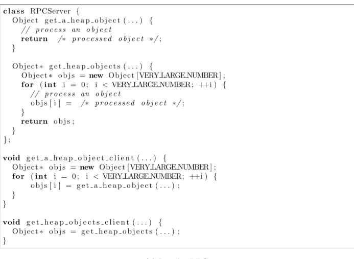
Consider the case of the GetHeapObjects function, which is supposed to send multiple objects back to the caller. Given the complexity of the application, there could be millions of objects to be sent back per request. A regular RPC implementation either sends back a single object, as in the get a heap object function, or a list of all objects, as in the get heap objects function in Figure 4.2a, per call. Unfortunately, both work terribly for our case, due to non-trivial overhead of millions of remote function calls per request or the massive memory consumption to cache all objects in memory before sending them back to the caller in batch.

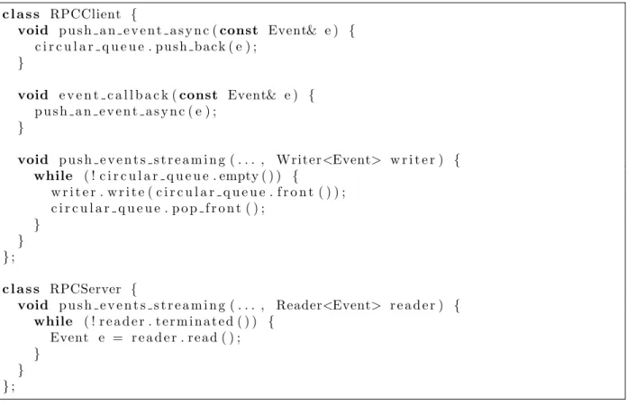
Our solution to this is to implement the streaming RPC that allows the callee to send responses back to the caller in a fashion similar to writing byte streams to a TCP connection, in this case however, writing objects one by one within a single RPC call. To terminate a streaming RPC call, the callee needs to write a terminator to the caller indicating the end of the response stream, and the caller needs to end the processing logics when a terminator is received. We show an example of Streaming RPC in Figure 4.2b.

Another case where regular RPC implementation does not play well is when a break-point callback needs to send an event notification to the callee, but has to be blocked until the return of the call, which also blocks the underlying Java application, slowing down its execution substantially. To solve this issue, we combine asynchronous RPC with stream-ing RPC that all events are first cached in a circular queue, which are later sent out usstream-ing streaming RPCs with separate threads.

We use asynchronous and streaming RPC extensively in our RPC service to reduce memory footprint and runtime overhead.

4.1.2 Interface Designs

We notice that information retrieved from JVMTI could be abstract and fragmented. For example, three functions need to called separately to get all information we need for a method, including the method id, name, and bytecodes. To simplify our RPC interface design, we organize those JVMTI functions into higher level RPC calls according to their logical functionalities, and group each fragmented information into structured messages as the parameters and return values of our interfaces. For clarity, we take theGetClassMethods interface as an example.

As mentioned earlier, getting all information of a method required three separate JVMTI function calls as shown in Figure 4.3a, however, for the simplicity of our RPC

(40)

c l a s s RPCServer { O b j e c t g e t a h e a p o b j e c t ( . . . ) { // p r o c e s s an o b j e c t return /∗ p r o c e s s e d o b j e c t ∗/; } O b j e c t∗ g e t h e a p o b j e c t s ( . . . ) {

O b j e c t∗ o b j s = new O b j e c t [VERY LARGE NUMBER ] ;

f o r (i n t i = 0 ; i < VERY LARGE NUMBER; ++i ) {

// p r o c e s s an o b j e c t o b j s [ i ] = /∗ p r o c e s s e d o b j e c t ∗/; } return o b j s ; } }; void g e t a h e a p o b j e c t c l i e n t ( . . . ) {

O b j e c t∗ o b j s = new O b j e c t [VERY LARGE NUMBER ] ;

f o r (i n t i = 0 ; i < VERY LARGE NUMBER; ++i ) {

o b j s [ i ] = g e t a h e a p o b j e c t ( . . . ) ; } } void g e t h e a p o b j e c t s c l i e n t ( . . . ) { O b j e c t∗ o b j s = g e t h e a p o b j e c t s ( . . . ) ; } (a) Regular RPCs

(41)

c l a s s RPCClient {

void p u s h a n e v e n t a s y n c (const Event& e ) {

c i r c u l a r q u e u e . p u s h b a c k ( e ) ;

}

void e v e n t c a l l b a c k (const Event& e ) {

p u s h a n e v e n t a s y n c ( e ) ;

}

void p u s h e v e n t s s t r e a m i n g ( . . . , Writer<Event> w r i t e r ) {

while ( ! c i r c u l a r q u e u e . empty ( ) ) { w r i t e r . w r i t e ( c i r c u l a r q u e u e . f r o n t ( ) ) ; c i r c u l a r q u e u e . p o p f r o n t ( ) ; } } }; c l a s s RPCServer {

void p u s h e v e n t s s t r e a m i n g ( . . . , Reader<Event> r e a d e r ) {

while ( ! r e a d e r . t e r m i n a t e d ( ) ) { Event e = r e a d e r . r e a d ( ) ; } } }; (b) Asynchronous Streaming RPC

(42)

interfaces, we provide one GetClassMethods function that extracts all the information from the JVM and group them into a single structured message that contains the ids, names and bytecodes of a method. That said, our GetClassMethods interface takes a re-quest from the caller indicating the classes, of which, the methods are to be extracted. It then iterates through and calls GetClassMethods on each of the classes to get a list of

method ids, and subsequently callsGetMethodName andGetBytecodes on each method of

each class. Before sending those information back to the caller, it wraps them into a list of JavaMethod structs, each containing the method id, name, and bytecodes of each method of each class. We show an abstract implementation of this process in Figure 4.3b. Note that besides omitting trivial syntaxes, the abstract implementation also shades the use of Protocol Buffer and gRPC for clarity.

The Xtract RPC service is implemented with the gRPC and Protocol Buffer framework. To define a gRPC function stub, one needs to provide a function signature, including the function return type, function name, as well as RPC request and response message types, among which, those types must be defined as Protocol Buffer messages. A Protocol Buffer message, referred to as a proto in later sections, is a language-independent structured message defined in .proto files. One can specify fields in a proto message, each of which could be a primitive, another proto message, or a repetition of primitives or proto messages. The gRPC function stubs and proto messages could be later compiled into the source files of various languages, including C/C++, Java, and Golang, that are used throughout our system. We describe our core interfaces and protos in AppendixA.

It is worth noting that most Xtract RPC interfaces produce XtractStatus as the re-sponse. XtractStatus is a proto message that describes whether a request is successful, and the error code and error message in the presence of request failures, however, it is to be distinguished from theStatus object returned by the gRPC framework. We briefly discuss this by first showing a compiled C++ function signature of SetBreakpoints as follows,

S t a t u s S e t B r e a k p o i n t s ( S e r v e r C o n t e x t∗ c o n t e x t , const

M u l t i p l e S e t B r e a k p o i n t P a r a m s∗ r e q u e s t , X t r a c t S t a t u s∗ r e s p o n s e ) ;

In the C++ function, the XtractStatus defined as the return type in Figure A.2a has been made one of the function parameters named response, while the return type of the function isStatus. TheXtractStatus is a custom proto message sent by Xtract to show any internal errors that may occur during invocations of the JVM APIs, while theStatus object generated and returned by the gRPC framework indicates whether or not the request failed due to a network or gRPC framework failure. As a client of the Xtract RPC service, both of these objects need to be inspected in the presence of failures to reason the cause.

(43)

// 1 . Get a l i s t o f methods g i v e n a c l a s s o b j e c t

j v m t i E r r o r GetClassMethods ( jvmtiEnv∗ env , j c l a s s k l a s s , j i n t∗

m e t h o d c o u n t p t r , jmethodID∗∗ m e t h o d s p t r ) ;

// 2 . Get t h e name o f a method g i v e n t h e method i d a c q u i r e d i n s t e p 1

j v m t i E r r o r GetMethodName ( jvmtiEnv∗ env , jmethodID method , char∗∗ name ptr ,

char∗∗ s i g n a t u r e p t r , char∗∗ g e n e r i c p t r ) ;

// 3 . Get t h e b y t e c o d e s o f a method g i v e n t h e method i d a c q u i r e d i n s t e p 1

j v m t i E r r o r G e t B y t e c o d e s ( jvmtiEnv∗ env , jmethodID method , j i n t∗

b y t e c o d e c o u n t p t r , unsigned char∗∗ b y t e c o d e s p t r ) ;

(a) Three Steps towards the Details of a Java Method with JVMTI

s t r u c t JavaMethod {

jmethodID m e t h o d i d ; s t d : : s t r i n g method name ;

unsigned b y t e∗ b y t e c o d e s ;

JavaMethod ( . . . ) { /∗ p a r a m e t e r i z e d c o n s t r u c t o r ∗/ }

}; // s t r u c t u r e d message c o n t a i n i n g r e q u i r e d i n f o r m a t i o n o f a Java Method

i n t GetClassMethods (const s t d : : v e c t o r<j c l a s s>& k l a s s e s , s t d : : v e c t o r<

JavaMethod>∗ m e t h o d s i n f o ) {

// l o c a l v a r i a b l e s d e c l a r e d h e r e

f o r (auto& k l a s s : k l a s s e s ) {

env−>GetClassMethods ( k l a s s , . . . , &m e t h o d i d s ) ;

f o r (auto& m e t h o d i d : m e t h o d i d s ) {

env−>GetMethodName ( method id , &name , . . . ) env−>G e t B y t e c o d e s ( method id , . . . , &b y t e c o d e s )

m e t h o d s i n f o−>e m p l a c e b a c k ( method id , name , b y t e c o d e s )

} }

// c l e a n up h e r e }

(b) Xtract Abstraction of GetClassMethods

(44)

4.1.3 Case Study

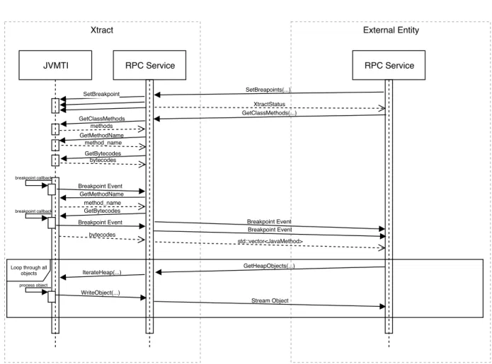
Figure 4.4: Sequence Diagram of the Xtract RPC Service, an Example

As a wrap up of this section, we present a sequence diagram of the Xtract RPC Service showing an example of asynchronous event pushing, object streaming, with an simultaneous invocation of GetClassMethods as in Figure 4.4.

Supposing the event management mechanism of this JVM is properly setup with the breakpoint event enabled. The external entity first sends aSetBreakpoints request through the RPC service, Xtract invokes correspondingSetBreakpoint function provided by JVMTI for each of the breakpoints specified in the RPC request. Upon return of the function, an XtractStatus indicating whether the function call is successful is return to the caller. Note that, with breakpoints set, JVMTI would now invoke breakpoint event callback before the execution of the instruction at which a breakpoint is set, which would send a event push

(45)

request to the RPC service, which would then send the breakpoint event to an external entity. After setting the breakpoints, the external entity now calls the GetClassMethods function.

Upon reception of the request, Xtract first gets a list of method ids for each class contained in the request. It will then get the name and bytecodes for each of those methods. After getting the bytecodes for the first method, JVMTI invokes the breakpoint callback which sends a breakpoint event to the RPC service. Note that the push operation is asynchronous that the callback function returns immediately without having to wait for the actual RPC call, which happens after the secondGetBytecodes function in this case.

An event notification may also happen between consecutive JVMTI calls, as for the case of the second breakpoint event, however, these operations should never block each other with the exception that if the event happens to stop the world or the thread one may be trying to access. The RPC service organizes those information into a list of JavaMethod messages and send it back to the caller. Lastly we show the sequence of streaming RPC with the example of GetHeapObject. The caller sends a request to get heap objects from the JVM, for which the RPC service initializes a heap walk, and writes objects back to the stream one by one, whenever they are processed. Note that this is a simplified depiction of the process showing the work flow of a streaming RPC, while the implementation details are discussed in Section 4.2.

4.2 Xtract JVMTI agent

The Xtract JVMTI agent implements the JVMTI APIs and is compiled as a shared library that could be loaded by a Java Virtual Machine. Backgrounds in terms of what is, and how to use JVMTI is discussed in Section 2.3, however, in this section, we discuss how Xtract retrieves runtime data from the JVM with JVMTI and JNI, including, breakpoints resolution and stack local variables inspection.

We discuss each of these implementations in the following sections.

4.2.1 Breakpoints Resolution

A breakpoint is set on a method instruction. The thread will be paused before the execution of the instruction at which a breakpoint is set, and an event notification will be sent through an event callback function that reports the id of the thread, and the location of

(46)

the instruction that the thread is about to execute. To set a breakpoint, a call to the SetBreakpoint function needs to be made with the id of the method and the location of the instruction to set the breakpoint.

Setting a breakpoint with Xtract involves the invocation of two interfaces, GetClass-Methods and SetBreakpoint. The first interface gets back a list of class methods, including their bytecodes, while the second interface sets a JVMTI breakpoint on a method bytecode instruction location. This way, we separate the determination of where to set a breakpoint entirely from the Xtract agent, and make it a decision of the external entity.

One breakpoint event notification sends one correspondingJvmEventNotification mes-sage to the external entity. The mesmes-sage contains the timestamp when the breakpoint callback is invoked, thread id, the name and id of the method, the name of the class that defines the method, and the location of the instruction at which the breakpoint event is triggered.

The message also includes a list of local variables available at the point of execution, used to derive local variable changes, which we now describe in the next section.

4.2.2 Stack Local Variables Inspection

Although desirable, the current latest version of JVMTI (JVMTI 1.2) does not provide approaches to set watchpoints on local variables [16, 25].

As a workaround, we implement Java local variable watchpoints with breakpoints, on instructions that change the values of local variables that we refer to as key instructions. For our case, we focus on the use of istore, lstore, fstore, dstore, and astore, that change the values ofinteger, long, float, double primitives, and object references respectively.

Note that, each of the instructions is presented in two possible forms.

• The short form uses a single instruction to access a value to a local variable slot, however, it only supports accessing values to local variable slot 0-3.

• Any operations that accesses the value of a local variable in slot greater than 3 adopts the long form that is expressed using two instructions with the first instruction being the op code, and the second being the slot number.

Breakpoints events are notified before the execution of an instruction, therefore, to get an event notification after a variable has been changed, a breakpoint should be set at

Anomaly Detection and Fault Localization Using Runtime State Models