Optimal Set of Multiple Relays and Distributed Self Selection in Cooperative Networks

(1)

Optimal Set of Multiple Relays and Distributed

Self-Selection in Cooperative Networks

Xiaohua Li, Chengyu Xiong, Jeong Kyun Lee

Department of Electrical and Computer Engineering, State University of New York, Binghamton, USA Email: [email protected], [email protected], [email protected]

Received March 15, 2013; revised April 15, 2013; accepted May 7, 2013

Copyright © 2013 Xiaohua Li et al. This is an open access article distributed under the Creative Commons Attribution License, which permits unrestricted use, distribution, and reproduction in any medium, provided the original work is properly cited.

ABSTRACT

In this paper we derive analytically the optimal set of relays for the maximal destination signal-to-noise ratio (SNR) in a two-hop amplify-and-forward cooperative network with frequency-selective fading channels. Simple rules are derived to determine the optimal relays from all available candidates. Our results show that a node either participates in relaying with full power or does not participate in relaying at all, and that a node is a valid relay if and only if its SNR is higher than the optimal destination SNR. In addition, we develop a simple distributed algorithm for each node to determine whether participating in relaying by comparing its own SNR with the broadcasted destination SNR. This algorithm has extremely low overhead, and is shown to converge to the optimal solution fast and exactly within a finite number of iterations. The extremely high efficiency makes it especially suitable to time-varying mobile networks.

Keywords: Cooperative Transmission; Amplify and Forward Relaying; Signal to Noise Ratio; Distributed Algorithm; Linear-Fractional Programming

1. Introduction

Cooperative communication has attracted great attention because it can exploit redundant communication nodes to enhance transmission performance. The general idea is to use these nodes to achieve the benefits of antenna array or multi-hop transmissions. Some cooperative transmission techniques have already been standardized in wireless networks such as the 4th Generation cellular systems and IEEE 802.16 m.

Although cooperative communications have received extensive investigation, some fundamental issues remain challenging. One of such issues is how to select relays optimally from all available redundant nodes. Another issue is how to implement such selection efficiently in a distributed environment. For the first issue, there are many important results published on single-relay selection [1,2]. In contrast, the multiple-relay selection problem, i.e., finding the optimal set of relays from a large group of candidates, is more challenging [3-10].

There have been extensive research on the performance of multiple relays [11-17], such as the outage capa- city or the optimal power allocation of fixed number of relays. As to the challenge of optimal relay set selection, for a special two-phase dual-hop relaying network with amplify-and-forward (AF) relaying, it has been shown in

[5] that all the nodes should be used as relays for an optimal transmit-beamforming-like cooperative transmission if perfect global channel state information (CSI) is available. Under a less stringent assumption (specifically, without global CSI, without perfect synchronization among nodes, etc.), it has been shown in [10] that only some nodes should participate in relaying.

For the issue of implementing relay selection, many existing cooperation schemes are based on centralized optimization algorithms, where all the nodes have to send their information to a central node. Obviously, this may suffer from big overhead, large delay, as well as reliabil- ity/security issues, in particular in highly mobile networks [13], or networks with high cost of feedback [16] and synchronization [17].

(2)

among the nodes. It is still an open problem as to how to implement the relays selection in a distributed yet efficient manner.

In this paper, we address the two issues by first ana- lyzing and simplifying the rules of the optimal selection of multiple relays in wireless networks with frequency selective fading channels. Then, we propose an efficient distributed algorithm with which each candidate node can determine by itself whether to participate in relaying. We will show that this algorithm can guarantee a rapid convergence within a finite number of iterations to the optimal solution, and has extremely low overhead.

The organization of this paper is as follows. In Section 2, we give the system model. In Section 3, we develop the optimal relay selection and propose the distributed algorithm. Simulations will be conducted in Section 4 and the conclusion will be given in Section 5.

2. System Model

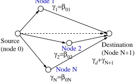
We consider a wireless ad-hoc network with a source node (Node 0), a destination node (Node ), and other nodes that can potentially work as relays, as illus- trated in Figure 1. The edge

1

N N

 

i j, from the node to the node has discrete frequency-selective fading

i j

channel g hij ij

 

n where gij is the power gain where-

as is the random channel coefficient with unit

gain, i.e.,

 

ij

h n

 

2

1

 

ij n

E h_ n 



where E

 

 denotes ex- pectation. We consider the linear time-invariant channels in this paper. But the results can also be applied when the channels are slowly time-varying. The maximum transmission power of each node is i Pi. Note that different

nodes can have different maximum transmission powers. We adopt the two-phase dual-hop relaying scheme. During the first phase, the source node broadcasts the signal s n

 

to all the other nodes. Then all the nodes selected as relays transmit their received signals to the destination node during the second phase. The destination node will combine the received signals during these two

=β

Source

(node 0) Node 2

Node N

Destination (Node N+1) γ1 01

Node 1

γΝ=β0Ν

γ2=β02 _γ

[image:2.595.101.242.589.674.2]

d+γΝ+1

Figure 1. Dual-hop cooperative wireless network with candidate relay nodes, each with SNR

N

i

 which equals to the “nominal edge SNR” 0i after optimization. The des-

tination node has SNR _d_N_₁.

phases for demodulation. We omit the details of the mo- dulation and demodulation. But rather, we focus on ana- lyzing the SNR of the received signals.

During the first phase, the signal received by the node , for

i i1,,N1 (including the destination node), is

 

0 01

 

0

 

,

i i i i

x n  g P s n h n v n (1) where P01P0 is the source node’s transmission power

during the first phase, v ni

 

is additive white Gaussian

noise (AWGN) with zero-mean and variance i2. We use

 t denote convolution. Assume the signal o s n

 

unit power. The power of the received signal

has

 

i

x n is thus

 

2 ₂

0 01

i i

E x n   g P i (2)

In this phase, the SNR of each receiving node i is

01 0

2 , 1, , 1

i i

i P g

i N

 

    (3)

During the second phase, the relays conduct amplify- and-forward (AF) cooperative transmissions. Each relay amplifies its received signal and transmits the following amplified signal

 

2

 

i i

i P

i s n

E x n



 

 

 

x n (4) where PiPi is the actual relaying (transmission) power.

We let Pi0 for those nodes that do not participate in

relaying. Note that the transmitted signal s ni

 

includes

both information signal s n

 

and noise . In this sense, not all candidate nodes may work as relays, and relays may not transmit at their full transmission power.



i

v n



We consider the case that the relays are not synchro- nized with each other in time. Each relay may have a unique (and random) delay i N, 1

i

 _ when transmitting to the destination node. Therefore, the destination node’s received signal is

 









 

, 1 , 1 , 1 , 1 0

d N

i N i i N i N i N d i

x n

g  s n   h  n   v n





    (5)

where we use

 

_d to make the variables different from the corresponding variables

 

_N_₁ of the destination node

 1

N in the first phase (1)-(3). We allow the source node to transmit again in this phase, and its transmitted signal is denoted as

 

0 02 ,

s n  P s n (6) where P02P0 is the source node’s transmission power

(3)

framework. If it does not happen, then we can just let

02 to remove its effect from all the results derived

in this pape 0

P 

r.

With our AF transmission, the relaying nodes do not need to estimate channels or to conduct demodulation. The relay nodes do not have to synchronize timing with each other either. This greatly reduces the cooperation overhead. This is in contrast to many other cooperative relaying setting, in particular to the transmit-beamforming- based cooperation scheme such as [4,5]. To realize transmit beamforming, each relay has to know both its receiving channel and its transmitting channel, and has to guarantee perfect timing synchronization with other relays. To acquire the transmitting channel knowledge, it needs the feedback from the destination node. Perfect timing synchronization among all the relays is even more costly, especially in dynamic mobile networks. As a result, although transmit-beamforming can achieve the highest destination SNR, the cost of cooperation overhead in ac- quiring perfect channel information and synchronization may compromise such a gain to a large extent. Under this consideration, the less stringent channel and timing synchronization requirement in our AF cooperative framework is in fact one of the special advantages. Later, we will show that our framework also leads to more succinct relay optimization rules and more efficient distributed algorithm implementation.

From (5), (4) and (1), the destination node’s received signal xd

 

n in the second phase is a mixture of the in-

formation signal s n

 

and the noises of all the relaying nodes and the destination node

 

















 









 

, 1 ₂ 0 01 , 1 1

d N

i

N

i x n





0 , 1 , 1 , 1 0, 1 02 0, 1

, 1 ₂ , 1

1

, 1 , 1 .

i

i N i i N

i

i i N i N i N

N N

i

i N i i N

i

i N i N d P

g g P s n

E x n

h n h n

g P s n

P

g v n

E x n

h n v n



 



 

  

 

 

 

 

 

   

 

 

 

 

  

(7)

We assume that all AWGNs i are independent

from each other and from the source signal

 

v n

 

s n . With- out loss of generality, we also assume that the random channel coefficients ij and the random propagation

delays i N, 1

 

h n

  are sufficiently mutually independent. Then, we can derive the SNR of the signal xd



t



in (7) as

, 1 2 0 01 0, 1 02 1 0 01

2 2 , 1 2 1 0 01

,

N

i

i N i N

i i i

N

i

i N i d

i i i

d

P

g g P g P

g P P g

g P



 



 



 

 



 



 (8)

where d2 is the noise power of the destination in the

second phase. We assume d2N21 for notational sim-

plicity, although our results can be easily extended to in- clude the other case.

The destination node can use the optimal maximum ratio combining (MRC) to combine the signals xN1

 

n in

(1) and xd

 

n in (5) received during the two phases.

From (3) and (8), the overall destination SNR is thus

1.

d N

   _ (9)

The multiple-relay selection problem can be formulated to maximize (9) by choosing appropriate transmission powersPi, for i1,,N, i.e.,

0

arg max . i i P P

  (10)

If P_i0, then the node is not selected as relay. Note that from (3) and (8) it is easy to see that the source node should always transmit at full power, i.e.,

i

01 02

P P P0, in both phases, in order to maximize the

destination SNR .

3. Optimal Selection of Relays

3.1. Optimal Relays and Destination SNR

To simplify the notation, we define the ratio of each node’s transmission power to its maximum available transmission power as

, 1, , .

i i

i P

z i

P

   N

1

(11)

Then 0 z_i

01 02 1

z z

. Note that for the source node we have   . We define

2

i ij ij

j P g

 

 (12)

as the nominal SNR of the edge

 

i j, when the node transmits at full power to . Because the source node always transmits at full power in the first phase, the received signal’s SNR of each node equals to the nominal SNR, i.e.,

i j

i

0, 1, , 1.

i i i N

     (13)

Following [10], after some straight-forward deductions we can rewrite (8) into

, 1 0, 1 0

1 0 , 1 1 0

1

, 1

1

N

i N

N i i

i i

d N

i N i

i i

z z



 



 _

  





 

 

 



(14)

and the overall destination SNR is   d 0,N1. The

optimal relay selection problem (10) is thus reduced to



: 1, ,



arg max_₀ ₁_ .

i

i d

z

z i N 

 

(4)

The optimization (14)-(15) is a linear fractional programming, which can be solved by many efficient linear programming algorithms [18]. Nevertheless, closed-form solutions are more desirable if available. For this purpose, we notice that the optimization problem (15) is similar to that of [10], even though in this paper we have consid- ered the more general frequency-selective fading channels and have allowed the relay nodes to have different maximum transmission powers.

Considering the optimization results of [10], we can immediately obtain the following optimal resolution to (15)

, 1

0 0 0 0,

1 0 1, if 1 0, otherwise N j N

j i i N

j j i z        _ 1            _{ }    



(16)

where the function

 

xmax 0,

 

x . (17) For each node, we can use (16) to determine whether it should participate in relaying, and to determine the asso- ciated relaying power. The optimal solution shows that each node either relays with full transmission power or does not participate in relaying, i.e., or 0 only. There is no fractional . Such a result has great sig- nificance in practice because we do not need to pay extra efforts to determine the optimal transmission power for each node.

1 i

z

i

z

It is easy to verify that the function

 

, 1

0 0

1 1 0

N

j N j

j j

,N 1

f x  x  



 _

 

 





_  _{ }  x (18)

is monotony non-increasing for . Because and

0

x

0

 

0 0

f  lim_x_ f x

 

 , there exists an x such that f x

 

 0. Therefore, if ₀_ix, then we have . Considering the condition in (16), we find that all the nodes with

 

0i 0

0i

f 

x

 _ 

k

should be selected as relays. What is more, if a node is a relay (i.e.,

0

k k x

 

i k



 ), then all the other nodes with larger SNR   must be relays as well because 0i i x



  . We define all the nodes satisfying 0i x



 as valid relay, and the other nodes as invalid relay since they should not be selected as relays.

Define the node set

 

k 



i:0i0k,i1,,N



I (19)

which in fact includes all the nodes with SNR no less than that of the node k. Assume that the node K is the valid relay with the smallest SNR

0

K K

   

among all the valid relays. Then the optimal overall SNR of the destination is  d N 1

 



  where

 

, 1 1 , 1 1 . 1 1 i N N i i i K d i N i i K      _              



I I (20)

As extreme cases, if

1 1

max i N ,

i N  

   (21)

then there is no valid relay, and the overall SNR is

1

2 N

   _ . On the other hand, if









1 , 1 1 1 , 1 1 1 min , 1 1 N

N j j N j

j

i N

i N

j N j

j                   



(22)

then all nodes are valid relays.

Unfortunately, (16) needs all nodes’ information (or global CSI) in a complex way to determine whether a node is valid relay. This is obviously inconvenient and costly for real implementation. We prefer more efficient, and especially distributed implementation, of the relay nodes selection. For this purpose, we need better relay selection rules. Fortunately, the following result shows that the task can be simplified to just compare a node’s SNR to the destination SNR instead.

Proposition 1. A node k is valid relay, i.e.,

 

kI K , if and only if k d   k

.

Proof. First, if a node is valid relay, we have

0 0

k k K

    and we need to prove k d 

 . Con- sider the node K and the condition in (16). We have

, 1

0 ₀ ₀ 0

1 0

, 1

N

i N

i _K _K N

i i          _         _{ }



, 1 (23)

which can be easily changed to

 

, 1 , 1

0, 1 0 ₀

0 0

1 .

1 1

i N i N

N i _K

i i

i K i K

                           



I I (24)

Because 0,N1N1 and 0ii for any , we

can rewrite (24) into

i

 

, 1 1 0 , 1 1 . 1 1 i N N i i i K K i N i i K      _              



I I (25)

This is in fact just

0K d

 . Therefore

0K

k d

   . Next, if k d



 , we need to show that the node is a valid relay. Assume instead. Considering the fact

k



(5)

, 1

1

k N k

k d

k N k

 



 _

 



  



(26)

and combining it with (20) (by adding nominator with nominator, and adding denominator with denominator), it is easy to show that

 

, 1 , 1

1

, 1 , 1

1 1

.

1

1 1

k N i N

k N i

k i K i

d

k N i N

k i K i



   

 



 

 



 

 

 

  

 

 

 

 





 

 

 

 

 



I

 _

 (27)

According to (14), the Equation (27) means that using the node as an extra relay (i.e., the relay set is now ) can further increase destination SNR, a contradiction to the fact that

k



K



k



I

d



is maximum. The proposition is thus proved.

3.2. Distributed Iterative Algorithm

The Proposition 1 shows that the optimal destination SNR d



during the second phase can be a sole thre- shold to determine whether a node is valid relay. No other information, especially other candidate nodes’ information, is needed. Therefore, the candidate nodes do not have to share information by handshaking. This can greatly reduce the cooperation overhead.

However, the problem is that d 

is available only after all the optimal relays have been selected. Fortu- nately, this “chicken-and-egg” dilemma can be resolved in practice thanks to the following proposition.

Proposition 2. If a mixture of valid and invalid relays are participating in relaying, the following holds:

1) Adding an extra valid relay can further increase destination SNR;

2) If the invalid relay has the smallest SNR  

among all the current relaying nodes and all the nodes in are participating in relaying, then the destination SNR

 

 I

d

 _.

Proof. The Statement 1) can be proved easily following (26) and (27) because any valid relay has SNR larger than d



. We can prove the Statement 2) by contradiction. Assume  d instead. First, the destination

SNR is





now

 

, 1 1

, 1

1 . 1

1 i N

N i

i I i

d

i N

i I i



 



 _

  









 

 





(28)

The Equation (28) can be changed to





 

, 1

1.

1 i N

i d d N

i I i



   

 

 

  







(29)

Replacing i by 0i, and because d0, we

obtain





 

, 1

0 0 0 0, 1 0

. 1

i N

i N

i i



   

 

 

  





 



I (30)

Since all the nodes in are participating in relaying, the Equation (30) can be re-written as

 

 I





, 1

0 0 0 0, 1

1 0

. 1

N

i N

i N

i i



   

  

 

  





  (31)

According to (16), we find that the node is a valid relay, which is a contradiction to the fact that the node is an invalid relay.



The Proposition 2 indicates that a node i can determine by itself whether to participate in relaying by comparing its received signal’s SNR i to the desti-

nation’s current SNR d of the second phase. If it is a

valid relay, it will increase d further by joining in re-

laying. Otherwise, its SNR will be smaller than the destination SNR. This is extremely convenient for distributed implementation, because we just require the destination node to periodically broadcast its SNR. There is no need of any other handshaking among the nodes or the feedback of channel information from the receiving nodes to the transmitting nodes. This drastically reduces the overhead and is also robust to dynamic change of the network caused by node movement or node failure.

We propose the following distributed iterative algorithm for the self-selection of multiple relays. With this algorithm, each node recursively estimates its probability

i

 

i

p t of participating in relaying, and determine whether participating in relaying according to this probability.

Distributed Algorithm for Self-Selection of Multiple Relays

During each iteration t0,1,,

1) The destination node estimates and broadcasts its SNR _d

 

t of the second phase;

2) Each node estimates its own SNR i _i

 

t , and participates in relaying with probability

 

min 1,





 





.

i i i d

p t  _c  t  t _ (32)

The parameters i are some appropriately chosen

constants. They can in fact be set identically to some large enough constant 0. We can initiate the algorithm

with a random selection of relays. The proof of the c

(6)

convergence of this distributed algorithm is as follows.

Proposition 3. Assume constant nodes SNR i

 

t i

and large enough constants . The algorithm converges to the optimal solution within iterations,

i.e., for , we have

1,

, ,

i

c i  N

 

d t d

N

tN   and

 

1, if

0, if

i i

i d

t p t

t d

 



 

  



 (33)

Proof. Assume that in the



th iteration some valid and invalid relays are relaying. In the th iteration, the destination node first broadcasts the new SNR

. For the valid relays , since i



1 t

t



1

d t

  i  _d, we have

. Then from (32) we have



i d t

  1



p ti

 

1 if



1



1

i d

   _i

Consider those invalid relays that relayed in the last iteration. If now, we have

t  c



is satisfied. i



1

i d t

   p ti

 

0

according to (32), which means they cease relaying. Then we just need to consider the group of invalid relays that are still relaying in this th iteration. Specifically, we consider the node with the smallest SNR in this group. Obviously,  . According to Proposi-

tion 2, in the next iteration we should have t





1

d t

  



 

d t

_ .

Therefore the node will stop relaying from the next iteration, i.e., . This procedure is repeated until all the nodes in this group are eliminated.





1



0 p t_  

Since at least one invalid relays is eliminated during each iteration, the algorithm needs at most iterations to converge to the optimal solution.

N



Rapid convergence is critical for this type of distributed algorithms because the overhead of SNR broad- casting and invalid relay transmission can be much reduced. In most cases our algorithm can in fact converge much faster than , or within much less than iterations, because in each iteration there are usually multiple candidate relays (rather than one) that can determine cor- rectly whether to participate in relaying. As a matter of fact, all valid relays and a big portion of invalid relays can be determined within the first several iterations. There are usually only a small portion of invalid relays within the third group (as specified in the proof of the Proposition 3), and more than one of them may be eliminated duration each iteration.

N N

This situation is especially true when the network is time-varying. For example, when some nodes leave or join the network, since the destination SNR is already in a high value, only several nodes may need to adjust their relaying status. This means the destination node needs to broadcast its SNR in-frequently, or even occasionally only. This makes our algorithm much more efficient than most of the centralized or existing distributed algorithms. In addition, the fast convergence makes our algorithm work effectively in time-varying environment, such as highly mobile wireless networks.

Our simulations indicate that a sufficiently large or works well. We can in fact just let

0

c

i

c

 

sign



 

,

i i d

p t _  t  t



_ (34) where sign

 

 is the signum function. Note that in this case, the algorithm becomes a deterministic algorithm because no probability of relaying is actually involved.

Nevertheless, using i with limited value provides us

a flexible way to control the contribution of valid relays. For those valid relays with very small i d

c

 _ 

, since their contribution to the destination SNR is small, some- times we may prefer to use some limited i to block

them from relaying. This special technique can be tailored to strike a balance between maximizing destination SNR and minimizing relay’s power consumption or other cri- teria.

c

In practical implementation, the destination node should broadcast the SNR at lower enough data rate in order for all the nodes to receive such information successfully, especially for those with small N1,i. On the other hand,

if a weak feedback channel N1,i means a weak for-

ward channel i N, 1 according to channel reciprocity,

the elimination of those valid relays with small i N, 1

does not degrade the destination SNR too much. There- fore, the destination node can use the broadcast data rate to block this type of nodes from relaying as well. These two special techniques may be applied jointly to adjust the number of relays selected in practice.

4. Simulations

We simulated a random wireless ad hoc network of 2

N nodes with relay candidate nodes. The nodes’ positions were randomly generated within a square of

N

1000 1000 meters. The nominal edge SNR was calcu- lated as ij where dij was the propagation

distance. Source and destination nodes were fixed with distance

8

10

 2.6

d

1000

ij



d0,N1 meters unless otherwise stated.

In the first experiment, we simulated our new algorithm (“Dist. Alg.”) and the optimal analytical results (20) (“Optimal”). Note that we stopped our new algorithm at just N1 iterations. We compared them with the schemes using a single optimal relay (“Single Relay”) [1] or using all the relay nodes (“Use All Node”) transmitting at full power. As performance measure, we consider the average of destination node’s SNR over randomly generated network setting. 10,000 runs of the simulations were conducted to find the average SNR. The simulation results in Figure 2 show that our distributed algorithm converges to the optimal solutions perfectly. Both the proposed distributed algorithm and the analysis results are correct. In addition, the optimal selection of all the valid relays has performance much better than either using a single relay or using all the relays non-optimally.

(7)

Next, for , we ran our distributed algorithm in 20 randomly generated networks and sketched the convergence of the destination SNR (normalized by the optimal SNR) in Figure 3. It can be clearly seen that our algorithm converges rapidly within about 6 iterations only. Note that it is much less than , the size of the network and the upper-limit of the convergence speed suggested in Proposition 3.

30 N

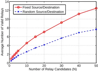
The average number of valid relays for random wireless networks with various number of relay candidates was simulated and shown in Figure 4. We simulated two different scenarios: fixed source/destination location, and randomly generated source/destination location. In the former case, since most of the relay candidates were

N

0 10 20 30 40 50

4 6 8 10 12 14

Number of Relay Candidates (N)

Average SNR (dB)

[image:7.595.340.505.88.205.2]

Dist. Alg. Optimal Single Relay Use All Nodes

Figure 2. Average destination SNR as functions of number of relay candidates.

5 10 15 20 25 30

0.4 0.6 0.8 1

Number of Iterations (t)

[image:7.595.92.251.268.381.2]

SNR (normalized by Optimal SNR)

Figure 3. Rapid convergence of the proposed distributed algorithm.

0 10 20 30 40 50

0 2 4 6 8 10 12 14

Number of Relay Candidates (N)

Average Number of Valid Relays

Fixed Source/Destination Random Source/Destination

Figure 4. Average number of valid relays in wireless net- works with various number of relay candidates.

0 20 40 60 80 100

Number of Candidate Relays (N)

Overhead: Number of Handshake Message

s

Dist. Alg.

[image:7.595.90.253.424.536.2]

Cooperative Beamforming: Zheng Network Beamforming: Jing Centralized

Figure 5. Cooperation overhead in wireless networks with various number of relay candidates.

in the middle between the source and destination, the average number of valid relays was relative higher. How- ever, in both cases, only a small portion of candidate nodes were valid relays.

Finally, we simulated the cooperation overhead of our proposed distributed algorithm under various number of relay candidates . We compared it to the “Central- ized” algorithm where each relay candidate broadcasted its own channel information to a central node. We also compared it to the other two distributed algorithms proposed in [4,5]. Except our algorithm, all the other three algorithms require channel estimation and channel information feedback. Note that the other three algorithms are not iterative algorithms. We assumed that the transmission of a parameter required a special handshaking message. We used the average number of message exchanges among the nodes as the cooperation overhead measure. The simulation results are shown in Figure 5. It clearly shows that the cooperation overhead of our proposed algorithm is much smaller, even less than

N

N , while all the other three algorithms are larger than . This dem- onstrates the extremely high efficiency of our proposed algorithm.

N

5. Conclusion

For a dual-hop amplify-and-forward cooperative network, we give analytical results of the optimal selection of all possible relays, and develop a distributed algorithm for multiple-relay self-selection. This algorithm is efficient with extremely low overhead, and can converge to the optimal solution rapidly within finite number of iterations. Simulations are conducted to verify the superior performance of the proposed algorithm.

REFERENCES

[image:7.595.87.256.581.703.2]

(8)

[2] D. S. Michalopoulos, G. K. Karaginannidis, T. A. Tsiftsis and R. K. Mallik, “An Optimized User Selection Method for Cooperative Diversity Systems,” Proceedings of IEEE GLOBECOM, San Francisco, 27 November-1 December 2006.

[3] Y. Li, P. Wang, D. Niyato and W. Zhuang, “A Dynamic Relay Selection Scheme for Mobile Users in Wireless Re- lay Networks,” Proceedings of 30th IEEE International Conference onComputer Communications (INFOCOM), Shanghai, 10-15 April 2011.

[4] G. Zheng, K.-K. Wong, A. Paulraj and B. Ottersten, “Col- laborative-Relay Beamforming with Perfect CSI: Opti- mum and Distributed Implementation,” IEEE Signal Pro- cessing Letters, Vol. 16, No. 4, 2009, pp. 257-260. doi:10.1109/LSP.2008.2010810

[5] Y. Jing and H. Jafarkhani, “Network Beamforming Using Relays with Perfect Channel Information,” IEEE Trans- actions on Information Theory, Vol. 55, No. 6, 2009, pp. 2499-2516. doi:10.1109/TIT.2009.2018175

[6] Y. Jing and H. Jafarkhani, “Single and Multiple Relay Se- lection Schemes and Their Achievable Diversity Orders,”

IEEE Transactions on Wireless Communications, Vol. 8, No. 3, 2009, pp. 1414-1423.

doi:10.1109/TWC.2008.080109

[7] G. Amarasuriya, M. Ardakani and C. Tellambura, “Adap- tive Multiple Relay Selection Scheme for Cooperative Wireless Networks,” IEEE Wireless Communications and Networking Conference, Sydney, 18-21 April 2010. [8] M. Choi, J. Park and S. Choi, “Low Complexity Multiple

Relay Selection Scheme for Cognitive Relay Networks,”

IEEE Vehicular Technology Society Conference, San Fran- cisco, 5-8 September 2011.

[9] H. Kartlak, N. Odabasioglu and A. Akan, “Adaptive Mul- tiple Relay Selection and Power Optimization for Cogni- tive Radio Networks,” Proceedings of 9th International Conference on Communications, Bucharest, 21-23 June 2012, pp. 197-200.

[10] X. Li, “Optimal Multiple-Relay Selection in Dual-Hop Amplify-and-Forward Cooperative Networks,” Electron-

ics Letters, Vol. 48, No. 12, 2012, pp. 694-695. doi:10.1049/el.2012.0194

[11] P. Larsson and H. Rong, “Large-Scale Cooperative Relay Network with Optimal Coherent Combining under Ag- gregate Relay Power Constraints,” Proceedings of Work- ing Group 4, WWRF8 Meetings, Beijing, February 2004. [12] I. Maric and R. D. Yates, “Bandwidth and Power Alloca-

tion for Cooperative Strategies in Gaussian Relay Net- works,” Proceedings of Asilomar Conference on Signals,

Systems & Computers, 7-10 November 2004, pp. 1907- 1911.

[13] M. Chen, T. C.-K. Liu and X. Dong, “Opportunistic Mul- tiple Selection with Outdated Channel State Information,”

IEEE Transactions on Vehicular Technology, Vol. 61, No. 3, 2012, pp. 1333-1345. doi:10.1109/TVT.2011.2182001 [14] S. Kim, J.-H. Park and D.-J. Park, “Beamforming of Am-

plify-and-Forward Relays under Individual Power Con- straints,” IEEE Journal on Selected Areas in Communica- tions, Vol. 30, No. 8, 2012, pp. 1347-1357.

doi:10.1109/JSAC.2012.120905

[15] M. Hong, Z. Xu, M. Razaviyayn and Z.-Q. Luo, “Joint User Grouping and Linear Virtual Beamforming: Com- plexity, Algorithms and Approximation Bounds,” IEEE Journal on Selected Areas in Communications, Special Issues on Virtual Antenna Systems, 2013.

[16] E. Koyuncu and H. Jafarkhani, “On the Structure of Lim- ited-Feedback Beamforming Codebooks for Amplify-and- Forward Relay Networks,” IEEE Transactions on Infor- mation Theory, Vol. 58, No. 5, 2012, pp. 2874-2895. doi:10.1109/TIT.2011.2179116

[17] X. Li, C. Xing, Y.-C. Wu and S. C. Chan, “Timing Esti- mation and Resynchronization for Amplify-and-Forward Communication Systems,” IEEE Transactions on Signal Processing, Vol. 58, No. 4, 2010, pp. 2218-2229. doi:10.1109/TSP.2009.2039837