Parallel Computation In Econometrics: A Simplified Approach
Jurgen A. Doornik∗, Neil Shephard & David F. Hendry, Nuffield College, University of Oxford, Oxford OX1 1NF, UK
January 30, 2003
Abstract Parallel computation has a long history in econometric computing, but is not at all wide spread. We
believe that a major impediment is the labour cost of coding for parallel architectures. Moreover, programs for specific hardware often become obsolete quite quickly. Our approach is to take a popular matrix programming language (Ox), and implement a message-passing interface using MPI. Next, object-oriented programming allows us to hide the specific parallelization code, so that a program does not need to be rewritten when it is ported from the desktop to a distributed network of computers. Our focus is on so-called embarrassingly parallel computations, and we address the issue of parallel random number generation.
Keywords: Code optimization; Econometrics; High-performance computing; Matrix-programming language; Monte Carlo; MPI; Ox; Parallel computing; Random number generation.
1
Introduction
There can be no doubt that advances in computational power have had a large influence on many, if not all, scientific disciplines. If we compare the current situation with that of 25 years ago, the con-trast is striking. Then, electronic computing was almost entirely done on mainframes, and primarily for number crunching purposes. Researchers, particularly in the social sciences, had limited budgets (often measured in seconds of computing time) and frequently had to schedule their computations at night. Moreover, the available software libraries were limited, and usually much additional program-ming was required (largely in FORTRAN, and still using punchcards). Today, a simple notebook has more power. In terms of research, the computer is used for a much wider range of tasks, from data management and visualization, to model estimation and simulation, as well as writing papers, to name a few. Most importantly, all access constraints have since disappeared.
Regarding high-performance computing (HPC), the situation, until quite recently, is more similar to that of 25 ago. Of course, systems are very much faster. But they are administered as mainframe systems, largely funded through physical sciences projects, requiring much dedicated programming. The current record holder (see www.top500.org) is the Japanese Earth Simulator. This supercomputer took five years to build, consists of 5120 processors, and is housed in a four story building with its own small power station. The machine is a parallel vector supercomputer, achieving 36 teraflops (a teraflop is1012floating point operations per second). In contrast, most other machines in the ranking are all massively parallel processor (MPP) and cluster machines, using off-the-shelf components: the second fastest is an MPP machine delivering nearly 8 teraflops. The gap is largely due to higher communication overheads in MPP architectures. In contrast, a current desktop reaches 2.5 gigaflops, equivalent to a supercomputer of the mid to late eighties. The speed difference between an up-to-date
desktop and the state-of-the-art supercomputer is of the order104. If Moore’s law continues to hold,1 it will take twenty years for the desktop to match the Earth Simulator.
Our interest lies in high-performance computing for statistical applications in the social sciences. Here, computational budgets are relatively small, and human resources to develop dedicated software limited (we consider this aspect in more detail in Doornik, Hendry, and Shephard, 2002). A feasible approach uses systems consisting of small clusters of personal computers, which could be called ‘personal high-performance computing’ (PHPC). Examples are:
• a small dedicated compute cluster, consisting of standard PCs;
• a connected system of departmental computers that otherwise sit idle much of the time. In both cases, hardware costs are kept to a minimum. Our objective is to also minimize labour costs in terms of software development. A fundamental aspect of these systems is that communication between nodes is slow, so they are most effective for so-called ‘embarrassingly parallel’ problems, where the task is divided into large chunks which can be run independently.
A prime example of an embarrassingly parallel problem is Monte Carlo analysis, whereM sim-ulations are executed of the same model, each using a different artificial data set. WithP identical processors, each ‘slave’ can runM/(P −1)experiments, with the ‘master’ running on processorP to control the slaves and collect the result. If inter-process communication is negligible, the speed-up is (P −1)-fold. The efficiency is100(P −1)/P%, i.e.85%when P = 7. In practice, such high efficiency is difficult to achieve, although improved efficiency results when the master process does not need a full processor.2 Many readers will be familiar with the manual equivalent: at the end of the afternoon, go to several machines to start a program, then collect the results the next morning. This procedure is efficient in terms of computer time, but quite error prone, as well as time consuming. Our aim is simply to automate this procedure for certain types of computation.
The 25 years of computing developments that are our time frame for comparison here have also resulted in a major transformation of the tools for statistical analysis in the social sciences. Then, there were quite a few ‘locally produced’ libraries and script-driven packages being used for teaching and research. Today, the default is to look for a readily available package. In econometrics, which is our primary focus, this would be PcGive or EViews for interactive use, and TSP, Stata or RATS for command-driven use.3 These have been around for a long time, and embody many years of academic knowledge. Such canned packages are often too inflexible for research purposes, but a similar shift has occurred in the move from low-level languages like FORTRAN and C, to numerical and statistical programming languages. Examples are MATLAB, GAUSS, Ox, S-plus, and R.4The labour savings in development usually outweigh the possible penalty in run-time speed. In some cases, the higher-level language can even be faster than the corresponding user program written in C or FORTRAN (for an Ox and GAUSS example, see Cribari-Neto and Jensen, 1997).
Parallel applications in econometrics have quite a long history. For example, one of the authors de-veloped Monte Carlo simulation code for a distributed array processor using DAP FORTRAN (Chong
1
Moore’s law predicts that on-chip transistor count doubles every 18 months. Such an improvement roughly corresponds to a doubling in speed. The ‘law’ accurately describes historical computer developments.
2In theory, there could be super-linear speed-up: e.g., when the distributed program fits in memory, but the serial version
does not.
3
Trademarks are: EViews by Quantitative Micro Software, PcGive by Doornik&Hendry, RATS by Estima, Stata by Stata Corp, TSP by TSP Intl.
4
Trademarks are: MATLAB by The MathWorks, Inc.; GAUSS by Aptech Systems Inc.; Ox by OxMetrics Technologies Ltd., S-PLUS by Insightful Corp., R see www.r-project.org.
and Hendry, 1986). The availability of low cost clusters has resulted in some increase in parallel appli-cations. For example, Swan (2003) considers parallel implementation of maximum likelihood estima-tion; Nagurney, Takayama, and Zhang (1995) and Nagurney and Zhang (1998) use massively parallel systems for dynamic systems modelling; Gilli and Pauletto (1993) solve large and sparse nonlinear systems; the monograph by Kontoghiorghes (2000) treats parallel algorithms for linear econometric models; Ferrall (2001) optimizes finite mixture models; examples of financial applications are Zenios (1999), Abdelkhalek, Bilas, and Michaelides (2001), and Pauletto (2001); Kontoghiorghes, Nagurney, and Rustem (2000) introduce a special issue on economic applications.
We believe that more widespread adoption of PHPC in our field of interest depends on two factors. First, only a minimum amount of programming should be required. Second, any method should be built around familiar software tools. Our approach is to take the Ox matrix-programming language (see Doornik, 2001), and try to hide the parallelization within the language. This way, the same Ox program can be run unmodified on a stand-alone PC or on a cluster as discussed in§5.7. This approach is in the spirit of Wilson (1995, p.497), who argues for the adoption of high-level languages. He also states that a company called Teradata was one of the most successful parallel computer manufacturers of the 1980s because: ‘in many ways, Teradata’s success was achieved by hiding parallelism from the user as much as possible’.
Before considering parallel applications for PHPC, we need to address speed aspects of single-processor implementations. After all, it is pointless gaining a four-fold speed increase by using four computers, but then losing it again because the actual software is four times slower than other pro-grams. This potential drawback has to be balanced against the effort already invested in the slower software: in terms of development time, it may still be beneficial to use a parallel version of the slower software.
The outline of the remainder of the chapter is as follows. The next section discusses the benefits and drawbacks of using a matrix language, followed by a brief introduction to the Ox language. Then,
§4 looks at some relevant single processor performance issues. §5 has an extensive discussion of how distributed processing is added to Ox using MPI (message-passing interface). Important aspects include random number generation (§5.5) and hiding the parallelism (§5.7);§6 provides an application of PHPC. Finally,§7 concludes.
2
Using a matrix-programming language
2.1 Introduction
Matrix-programming languages have become the research tool of choice in many disciplines, because they make program development substantially easier. Computational expressions are much closer to algebraic statements, thus reducing the amount of coding required. Moreover, such languages usually come with substantial numerical and statistical libraries built-in.
Low-level languages like C, C++ and FORTRAN are translated into machine language by a com-piler, and saved as an executable image. Matrix languages are interpreted line-by-line as they are read by the interpreter. The latter is similar to a Basic or Java program (provided no Just-in-time compiler is used). The drawback of an interpreted language is that control-flow statements like loops can be very slow. The advantage is that the edit-run cycle is much more convenient.
2.2 An illustration of the benefits of a matrix language
The recent history of PcGive shows how language considerations have changed, and illustrates the benefits of using a matrix language. PcGive is an interactive econometrics package that is used at universities, central banks, and financial institutions. The first PC version was created in 1983/4 as a port of the mainframe FORTRAN code. The severe memory limitations of the early PC, and low quality of early PC FORTRAN compilers, made development very challenging. The FORTRAN version was extended over nearly ten years, until it had become unmanageable, and development of a new version written in the C language was started. The main benefit of switching to C was the flexibility of memory management: the size of data matrices could be determined at run-time, rather than compile time. Since then, the program has been rewritten from scratch again, with a separate interface component that is in C++, and the computational part and econometric dialogs largely in a matrix programming language. The high-level language used is Ox. There are two immediate benefits:
• Use of matrix expressions leads to shorter and much simpler code.
• Memory allocation/deallocation is automatically handled in Ox. This removes a frequent source of bugs.
The attempt to reduce complexity by layering has been a constant thread in computer development. Initially, computers were programmed in machine language. Assembly was one step up, but a large step forward was the introduction of compilers (such as FORTRAN), that automatically translate more human-friendly code into machine language. Ox is written in C, and runs a higher-level C-like language tailored for econometrics and statistics. This is done by compiling Ox code into an intermediate language, which is then interpreted. Table 1 lists the approximate number of lines of code of versions of PcGive. By dropping FORTRAN and Assembly, each subsequent version has become less complex than its predecessor, and therefore easier to maintain. The switch to Ox in the most recent version has been a particular improvement, as can be seen from the reduction in the number of lines of code.
Table 1: Number of lines of code for four versions of PcGive year FORTRAN Assembly C C++ Ox
V6 1989 24000 5000 1500 0 0
V7 1992 0 3000 19000 0 0
V9 1996 0 0 18500 6000 0
V10 2001 0 0 4000 6500∗ 4000
∗This code is actually part of Ox, and shared between various applications.
2.3 Advantages and drawbacks of matrix programming languages
Several benefits were already illustrated in the previous section. For most matrix languages they include:
• Code is platform independent;
• Speed improvements for matrix expressions;
• Faster edit-run cycle than compiled languages;
• Facilitates code sharing. The drawbacks can be:
• Slower speeds of loops and matrix indexing;
• Dependence on less predictable ‘producer’ (whether open source or closed source development team);
• Limitations to producing stand-alone (possibly commercial) versions. The speed aspect can work both ways, and is discussed in more detail in§4.
3
The Ox matrix language
3.1 Overview
Ox has a comprehensive mathematical and statistical library, and, although Ox is a matrix language, it has a syntax that is similar to C and C++ (and Java). Ox is a relatively young language, with a first official release in 1996. Despite this, it has been widely adopted in econometrics and statistics. Two contributing factors are that it is fast, and that there is a free version for academics (but it is not open source). Ox is available on a range of platforms, including Windows and Linux. For a recent review see Cribari-Neto and Zarkos (2003).
Ox is an interpreted language,5 with a commensurate speed penalty for unvectorized code such as loops. However, this speed penalty is noticeably less than in other comparable systems. Indeed, several reviewers have noted that their programs, after conversion to Ox, actually run faster than their original FORTRAN or C code. §4 will explain how this can happen.
Time-critical code sections can be written in FORTRAN or C, and added to the language as a dynamic link library. Because of the similarity of Ox to C, it is often convenient to do the prototyping of code in Ox, before translating it into C for the dynamic link library. All underlying standard library functions of Ox are exported, so can be called from the C code. An example of a library that is implemented this way is SsfPack (Koopman, Shephard, and Doornik, 1999).
The Ox language is also object-oriented, along the lines of C++, but with a simplicity that bears more resemblance to Java. This is aided by the fact that Ox is implicitly typed. There are several pre-programmed classes; the most important are the Modelbase class, and the Simulation class. The latter is of interest here: if we can make it parallel, without affecting its calling signature, we can make existing programs parallel without requiring recoding.
Speed, extensibility, availability and familiar syntax: these features together make Ox a good candidate for parallel development. There are other matrix languages which can be significantly slower, removing most, if not all, of the speed advance we are hoping to achieve. In the remainder, we largely use Ox to illustrate the issues in implementing a matrix language for parallel use.
5
3.2 Example
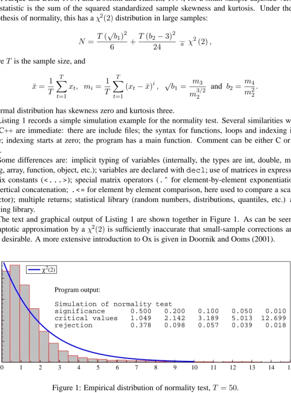
As a simple example of a simulation experiment in Ox, we take the asymptotic form of the univariate test for normality, the so-called Bowman-Shenton or Jarque-Bera test (see Bowman and Shenton, 1975, Jarque and Bera, 1987, and Doornik and Hansen, 1994, for a small-sample adjusted version). The statistic is the sum of the squared standardized sample skewness and kurtosis. Under the null hypothesis of normality, this has aχ2(2)distribution in large samples:
N = T( √b 1)2 6 + T(b2−3)2 24 a χ 2(2),
whereT is the sample size, and ¯ x= 1 T T t=1 xt, mi = T1 T t=1 (xt−x¯)i, √b1 = m3 m32/2 and b2= m4 m2 2.
A normal distribution has skewness zero and kurtosis three.
Listing 1 records a simple simulation example for the normality test. Several similarities with C and C++ are immediate: there are include files; the syntax for functions, loops and indexing is the same; indexing starts at zero; the program has a main function. Comment can be either C or C++ style.
Some differences are: implicit typing of variables (internally, the types are int, double, matrix, string, array, function, object, etc.); variables are declared withdecl; use of matrices in expressions; matrix constants (<...>); special matrix operators (.ˆfor element-by-element exponentiation, |
for vertical concatenation; .<=for element by element comparison, here used to compare a scalar to a vector); multiple returns; statistical library (random numbers, distributions, quantiles, etc.) and a drawing library.
The text and graphical output of Listing 1 are shown together in Figure 1. As can be seen, the asymptotic approximation by aχ2(2)is sufficiently inaccurate that small-sample corrections are in-deed desirable. A more extensive introduction to Ox is given in Doornik and Ooms (2001).
0 1 2 3 4 5 6 7 8 9 10 11 12 13 14 15 0.1 0.2 0.3 0.4 Program output:
Simulation of normality test
significance 0.500 0.200 0.100 0.050 0.010 critical values 1.049 2.142 3.189 5.013 12.699 rejection 0.378 0.098 0.057 0.039 0.018
χ2(2)
#include <oxstd.h> // include Ox standard library #include <oxdraw.h> // include Ox drawing library
NormTest1(const vX) // function with one argument
{
decl xs, ct, skew, kurt, test; // variables must be declared
ct = rows(vX); // sample size
xs = standardize(vX);
skew = sumc(xs .ˆ 3) / ct; // sample skewness
kurt = sumc(xs .ˆ 4) / ct; // sample kurtosis
test = sqr(skew) * ct / 6 + sqr(kurt - 3) * ct / 24;
return test | tailchi(test, 2); // [0][0]: test, [1][0]: p-value }
SimNormTest1(const cT, const cM, const vPvals) {
decl eps, i, test, tests, reject;
tests = new matrix[1][cM]; // create new matrix (set to zero) reject = zeros(1, columns(vPvals));//also new matrix of zeros for (i = 0; i < cM; ++i) // loop syntax is like C,C++,Java {
eps = rann(cT, 1); // T x 1 vector of std.normal drawings test = NormTest1(eps); // call the test function tests[i] = test[0];// stores actual outcomes for plotting reject += test[1] .<= vPvals; // update rejection count }
reject /= cM; // translate to frequency
return {tests, reject}; // return both values
} main() {
decl ct = 50, tests, reject;
decl pvals = <0.5,.2,.1,.05,.01>; // <..> is matrix constant decl time = timer(); // start timer and run experiment [tests, reject] = SimNormTest1(ct, 10000, pvals);
println("Simulation time: ", timespan(time));
DrawDensity( // draw the non-parametrically estimated density 0, tests,
sprint("Empirical distribution: normality test, T=", ct), FALSE, TRUE);
DrawXMatrix( // add the reference distribution
0, denschi(range(1,100)/10, 2), "$\chiˆ2(2)$", range(1,100)/10, "", 0, 3);
DrawAdjust(ADJ_AREA_X, 0, 0, 15);// cut fat tails from X-axis ShowDrawWindow();
println( // print selected quantiles (data is in rows) "Simulation of normality test",
"%r", {"significance", "critical values", "rejection"}, "%8.3f",
pvals | quantiler(tests, 1 - pvals) | reject); }
Listing 1: Example program for the univariate normality test
4
Single processor performance
4.1 Loops in matrix programming languages
A1 (see the Appendix). That function times a loop ofcRep iterations which calls a dot product functionvecmul. This in turn contains a loop to accumulate the inner product:
vecmul(const v1, const v2, const c) {
decl i, sum;
for (i = 0, sum = 0.0; i < c; ++i) sum += v1[i] * v2[i];
return sum; }
The corresponding C code is given in Listing A2. Of course, it is better to use matrix expressions in a matrix language, as in functionvecmulXtYvecin Listing A1. The speed comparisons (on a 1.2 Ghz Pentium III notebook running Windows XP SP1) are presented in Table 2. Clearly, this is a situation where the C code is many orders of magnitudes faster than the unvectorized Ox code. The table also shows that, as the dimension of the vectors grows, the vectorized Ox code catches up, and even overtakes the C code.
Table 2: Number of iterations per second for three dot-product implementations vector length 10 100 1000 10 000 100 000 unvectorized Ox code 67 000 8 900 890 89 9 vectorized Ox code 1 100 000 930 000 300 000 32 000 390 C code 15 000 000 3 200 000 330 000 34 000 380
In the extreme case, the C code is nearly 400 times faster than the Ox code. However, this is not a realistic number for practical programs: many expressions do vectorize, and even if they do not, they may only form a small part of the running time of the actual program. If that is not the case, it will be beneficial to write the code section in C or FORTRAN and link it to Ox. It is clear that vectorization of matrix-language code is very important.
4.2 Optimization of linear algebra operations
Linear algebra operations such as QR and Choleski decompositions underlie many matrix computa-tions in statistics. Therefore, it is important that these are implemented efficiently.
Two important libraries are available from www.netlib.org to the developer:
• BLAS: the basic linear algebra system, and
• LAPACK: the linear algebra package, see LAPACK (1999).
LAPACK is built on top of BLAS, and offers the main numerical linear algebra functions. Both are in FORTRAN, but C versions are also available. MATLAB was essentially developed to provide easier access to such functionality.
Several vendors of computer hardware provide their own optimized BLAS. There is also an open source project called ATLAS (automatically tuned linear algebra system, www.netlib.org), that pro-vides highly optimized versions for a wide range of processors. ATLAS is used by MATLAB 6, and can also be used in R. Ox has a kernel replacement functionality which allows the use of ATLAS, see the next section.
Many current processors consist of a computational core that is supplemented with a substantial L2 (level 2) cache (for example 128, 256 or 512 KB for many Pentium processors).6 Communication between the CPU and the L2 cache is much faster than towards main memory. Therefore, the most important optimization is to keep memory access as localized as possible, to maximize access to the L2 cache and reduce transfers from main memory to the L2 cache. For linear algebra operations, doing so implies block partitioning of the matrices involved.
For example, the standard three level loop to evaluateC=AB:
for (i = 0; i < m; ++i) for (j = 0; j < p; ++j) { for (k = 0, d = 0.0; k < n; ++k) d += a[i][k] * b[k][j]; c[i][j] = d; }
is fine whenAandB are small enough to fit in the L2 cache. If not, it is better to partitionA, Binto
Aij andBij, and use a version that loops over the blocks. EachAikBkjis then implemented as in the code above. The size of the block depends on the size of the L2 cache.
There are further optimizations possible, but the block partitioning gives the largest speed benefit.
4.3 Speed comparison of linear algebra operations
We look at the speed of matrix multiplication to show the impact of optimizations, using code similar to that in Listings A1 and A2, but this time omitting unvectorized Ox code.
We consider the multiplication of two matrices, and the cross-product of a matrix, for four designs:
operation A B for
AB r×r r×r r= 20(10)320
AA r×r r= 20(10)320
AB 50×c c×50 c= 10,100,1000,10 000,100 000
AA c×50 c= 10,100,1000,10 000,100 000
All timings in this section are an average of four runs.
Four implementations are compared on a Mobile Pentium III 1.2 Ghz (with 512KB L2 cache): 1. Vectorized Ox code.
This is the default Ox implementation. Note that Ox does not use BLAS or LAPACK. The Ox version is 3.2.
2. Naive C code.
This is the standard three-loop C code, without any block partitioning. We believe that this is the code that most C programmers would write.
3. ATLAS 3.2.1 for PIIISSE1
The SSE1 (version 1 streaming SIMD extensions) instructions are not relevant here, because they can only be used for single precision. All our computations are double precision.
6
4. MKL 5.2 (Intel)
The math kernel library (MKL) is a vendor-optimized BLAS (in this case, with a large part of LAPACK as well). This can be purchased from Intel, and is not available for AMD Athlon processors. We used the default version (for all Pentium processors), because it was regularly faster on our benchmarks than the Pentium III specific version.
Although each implementation is expected to have the same accuracy, the ordering of the summations can be different, resulting in small differences between outcomes.
The Ox, MKL, and ATLAS timings are all obtained with the same Ox program (Listing A4). Ox has the facility (as yet undocumented and unsupported) to replace its mathematical kernel library. This applies to matrix multiplications, eigenvalue and inversion routines, and Choleski, QR, and SVD (singular value) decompositions. Doing so involves compiling a small wrapper around the third-party BLAS/LAPACK libraries. This feature could also be used to implement parallel versions of these operations (such as, e.g., Kontoghiorghes, 2000), without the need to make any changes to Ox. A command line switch determines the choice of kernel replacement library.
20 60 100 140 180 220 260 300 1 10 100 1000 10000 → r ops/sec ops/sec
AB
C Ox+MKL Ox+Atlas Ox 20 60 100 140 180 220 260 300 1 10 100 1000 10000 → rA
′
A
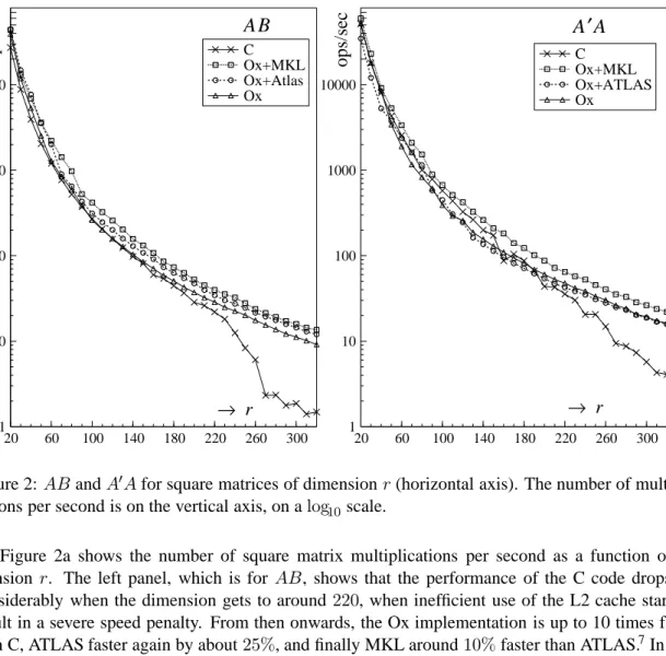
C Ox+MKL Ox+ATLAS OxFigure 2:ABandAAfor square matrices of dimensionr(horizontal axis). The number of multipli-cations per second is on the vertical axis, on alog10scale.
Figure 2a shows the number of square matrix multiplications per second as a function of di-mension r. The left panel, which is for AB, shows that the performance of the C code drops off considerably when the dimension gets to around 220, when inefficient use of the L2 cache starts to result in a severe speed penalty. From then onwards, the Ox implementation is up to 10 times faster than C, ATLAS faster again by about25%, and finally MKL around10%faster than ATLAS.7In this
7
design ATLAS outperforms Ox at all dimensions, whereas MKL is always faster than ATLAS. The symmetric case, Figure 2b, shows timings for the cross-productAAfor the same dimensions. The results are quite similar for large dimensions. At dimensions between 20 and 40, ATLAS is outperformed by all others, including C. From dimensions 90to150, the naive C implementation is faster than ATLAS and Ox, which could be due to overly conservative L2 cache use.
10 100 1000 10000 100000 0.1 1 10 100 1000 10000 ops/sec ops/sec → c
AB
C Ox+MKL Ox+Atlas Ox 10 100 1000 10000 100000 0.1 1 10 100 1000 10000 → cA
′
A
C Ox+MKL Ox+Atlas OxFigure 3:ABandAAfor matrices of dimension50×c(horizontal axis onlog10scale). The number of multiplications per second is on the vertical axis, on alog10scale.
The cases withr = 50andcvarying are presented in Figure 3. At large dimensions, the naive C code is again dominated, by a factor of 20forc= 100 000. In theABcase, Ox, MKL and ATLAS are quite similar, while forAA, Ox and MKL are twice as fast as ATLAS forc= 1000,10 000.
These examples show that speed depends very much on the application, the hardware and the developer. For example, on a Pentium 4, we expect ATLAS and MKL to more clearly outperform Ox, because they use SSE2 to add additional optimizations. The results show that matrix programming languages that have a highly optimized internal library can make some programs run faster than a low-level implementation in C or FORTRAN. It should also be clear that matrix languages embody a large range of relevant expertise.
The next sections considers what benefits arise for distributed computing using Ox, which has shown itself to be fast enough as a candidate for distributed processing.
5
Parallel implementation
5.1 Parallel matrix languages
There are several stages at which we can add distributed processing to a matrix language. Like low-level languages, it can be parallelized in the user code. Further, because there is an extensive run-time library, this could also be parallelized. Finally, the fact that a matrix language is interpreted creates an additional possibility: to parallelize the interpreter.
Here, we only consider making the parallel functionality directly callable from the matrix lan-guage. When a language can be extended through dynamic link libraries in a flexible way, this level can be achieved without changing the language interpreter itself. We would expect optimal perfor-mance gains for embarrassingly-parallel problems. Efforts for other languages are also underway: there is a PVM package for R, and Caron et al. (2001) discusses a parallel version of Scilab.
When the parallelization is hidden in the run-time library, operations such as matrix multiplica-tion, inversion, etc., will be distributed across the available hardware. Here we could use available libraries for the implementation (such as ScaLAPACK or PLAPACK, also see Kontoghiorghes, 2000). Functions which work on matrix elements (logarithm, loggamma function, etc.) are also easily dis-tributed. The benefits to the user are that the process is completely transparent. The speed benefit will be dependent on the problem: if only small matrices are used, the communication overhead would prevent the effective use of the cluster. The experience of Murphy, Clint, and Perrott (1999) is rele-vant at this level: while it may be possible to efficiently parallelize a particular operation, the benefit for smaller problems, and, by analogy for a complete program, is likely to be much lower. If a cluster consists of multi-processor nodes, then this level will be most efficient within the nodes, with the previous user level between nodes.8 This could be achieved using multi-threading, possibly using OpenMP directives (www.openmp.org).
Parallelization of a matrix language at the interpreter level is the most interesting implementation level, and, so far as we are aware, has not been tried successfully before. The basic idea is to run the interpreter on the master, handing elements of expressions to the slaves. The main problem arises when a computation requires a previous result – in that case the process stalls until the result is available. On the other hand, there may be subsequent computations that can already be done. This is an avenue for future research.
5.2 An MPI subset for Ox
We decided to add distributed processing to Ox using MPI (the message-passing interface), see Snir, Otto, Hus-Lederman, Walker, and Dongarra (1996) and Gropp, Lusk, and Skjellum (1999). This was not based on a strong preference over PVM (parallel virtual machine, see Geist, Beguelin, Dongarra, Jiang, Manchek, and Sunderam, 1994; and Geist, Kohl, and Papadopoulos, 1996, for a comparison of PVM and MPI). In PVM, child tasks are spawned from the parent, while in MPI the same single program is launched from the command-line, with conditional coding to separate the parent and child. The latter seemed slightly easier to implement within the Ox framework.9The objective here is not to provide a full implementation of MPI for Ox, although that can easily be done. Instead we just do what is sufficient to run an example program, and then extend this to distributed loops for embarrassingly parallel computations. §B.1 in the Appendix discusses how Ox is extended with dynamic link libraries, and§B.2 considers the MPI wrapper for Ox.
The first stage after installation of MPI (we used MPICH 1.2.5 under Windows, and MPICH 1.2.4 under Linux, see Gropp and Lusk, 2001), is to run some example programs. Column one of Listing 2 gives a simplified version of thecpi.cprogram as provided with MPICH. The simplification is to fix the number of intervals inside the program, instead of asking for this on the command line. The
8
Intel has introduced Hyperthreading technology on recent chips, where a single processor presents itself as a dual processor to increase efficiency.
9Certainly, under Windows it was relatively easy to get MPI to work with Ox. The main inconvenience is synchronizing
different computers if a network drive is not used for the Ox program and other files that are needed. However, under Linux, MPI uses a different mechanism to launch processes, involving complex command-line argument manipulations. This interferes with the Ox command line unless the Ox driver is re-compiled to incorporate the call toMPI Init.
#include "mpi.h" #include <stdio.h> #include <math.h> double f(double a) { return (4.0 / (1.0 + a*a)); } int main(int argc, char *argv[]) { int done = 0 , n , myid, numprocs, i; double PI25DT = 3.141592653589793238462643; double mypi, pi, h, sum, x; double startwtime, endwtime; char procname[MPI_MAX_PROCESSOR_NAME]; int namelen; MPI_Init(&argc, &argv); MPI_Comm_size(MPI_COMM_WORLD, &numprocs); MPI_Comm_rank(MPI_COMM_WORLD, &myid); MPI_Get_processor_name(procname, &namelen); printf("Process %d of %d on %s\n", myid, numprocs, procname); if (myid == 0) { n = 1000; startwtime = MPI_Wtime(); } MPI_Bcast(&n,1,MPI_INT,0,MPI_COMM_WORLD ); printf("id: %d n= %d\n", myid, n); h = 1.0 / (double) n; sum = 0.0; for (i = myid + 1 ; i <= n; i + = numprocs) { x = h * ((double)i -0.5); sum += f(x); } mypi = h * sum; printf("id: %d sum= %g\n", myid, sum); MPI_Reduce(&mypi, &pi, 1, MPI_DOUBLE, MPI_SUM, 0, MPI_COMM_WORLD); if (myid == 0) { printf("pi=%.16f, Error=%.16f\n", pi, fabs(pi -PI25DT)); endwtime = MPI_Wtime(); printf("wall clock time = %f\n", endwtime -startwtime); } MPI_Finalize(); return 0; } #include <oxstd.h> #include <packages/oxmpi/oxmpi.h> f(const a) { return (4.0 ./ (1.0 + a*a)); } main() { decl n, myid, numprocs, i; decl PI25DT = 3.141592653589793238462643; decl mypi, pi, h, sum, x; decl startwtime, endwtime; decl procname; MPI_Init(); numprocs = MPI_Comm_size(); myid = MPI_Comm_rank(); procname = MPI_Get_processor_name(); println("Process ", myid, " o f " , numprocs, " o n " , procname); if (myid == 0) { n = 1000; startwtime = MPI_Wtime(); } MPI_Bcast(&n, 0); println("id: ", myid, " n=", n); h=1 . 0 /n ; sum = 0.0; for (i = myid + 1 ; i <= n; i + = numprocs) { x = h * (i -0.5); sum += f(x); } mypi = h * double(sum); println("id: ", myid, " sum=", sum); pi = MPI_Reduce(mypi, MPI_SUM, 0); if (myid == 0) { println("pi=", "%.16f", pi, ", Error=", "%.16f", fabs(pi -PI25DT)); endwtime = MPI_Wtime(); println("wall clock time = " , endwtime -startwtime); } MPI_Finalize(); } Listing 2: MPI example program in C (left) and Ox (right)
second column of Listing 2 shows that the Ox implementation can be very similar. The MPI functions in their Ox version are:
MPI Init(); Initialize the MPI session. Can be called multiple times, unlike the original.
MPI Comm size(); Returns the number of processes. Within MPI, communications are asso-ciated with communicators which allow processes to be grouped into communication tasks. However, in the current implementation we assume thatMPI COMM WORLD, i.e. all processes, are the default communicator, and omit the argument to specify the communicator.
MPI Comm rank(); Returns the rank of the calling process.
MPI Get processor name(); Returns the name of the current processor.
MPI Bcast(const aVal, const iRoot); Broadcasts data from the sending processiRoot
to all other processes. So in all other processes than the sender,MPI Bcastoperates like the receiver. Ox types that can be broadcast are integer, double, matrix, string, and array. aVal
must be a reference to a variable, which on the sender must hold a value.
MPI Reduce(const oxval, const iOp, const iRoot); This performs an action on all the data on the processes other than root, and returns the result to root. In the example below, each non-root holds a part of the approximation to the integral expression for π. The sum is returned to root, to provide an estimate ofπ. MPI Reduceworks for integers, doubles and matrices.
MPI Wtime(); Returns the time in seconds since a time in the past (which is before the program started running).
MPI Finalize(); Terminates the MPI session. Unlike the original MPI version, this is an op-tional call, becauseMPI Initautomatically schedules a barrier synchronization and a call to
MPI Finalizeto be executed when the Ox interpreter finishes.
5.3 Parallel loops
The next stage is to use the MPI facilities to implement a parallel loop in the matrix language that we use. Here we also start using Ox’s object-oriented features, to facilitate the use of the loop code.
Ox follows a simplified version of the C++ object-oriented paradigm. In its most basic form, a class is a collection of functions and variables (both members of the class), which are grouped together. The variables are accessible to function members, but invisible to the outside world. A new class can derive from an existing class to extend its functionality; virtual functions allow a derived class to override base-class functionality. Finally, an object of a class is created with new for subsequent use (and, as an important improvement over programming with global variables, there can be many objects of the same class). For a more extensive introduction see Doornik and Ooms (2001), while a comparison of Ox syntax with C++ and Java is given in Doornik (2002).
To implement a parallel library in Ox, we adopt the master/slave model written in MPI: the same program is running on each node, withifstatements selecting the appropriate code section. Listing 3 gives an outline of the class. In this case, all members have been made static, so there can only be one instance running at a time: more than one would make the program very inefficient anyway. This also implies that there is no need to instantiate the class usingnew. The core is theRunfunction that runs a specified functioncReptimes.Initis called first to initialize the MPI library and the Loop class.
The master is the process with the highest rank (arbitrarily), and we have added theMPI SetMaster
andMPI IsMasterfunctions to the Ox MPI wrapper to facilitate tracking of master/slave status in the Ox code. The second argument ofMPI SetMasteris used here to switch off all output from the slave processes. Although much of the relevant code has been stripped away, allowance is made for this class to work outside MPI: in that case neitherIsMasternorIsSlaveis true.
TheRunfunction is the core of this Loop class, and usually the only one called. It initializes MPI and the class, then calls an optional loop initialization function on the slaves. Next, either the master or the slave version is called (or the non-MPIdoLoop). A final barrier synchronization ensures that all processes get to this point before continuing.
Runtakes three function arguments, in addition to the loop size:
fnInit to initialize the slave loops (optional);
fnRun to run a replication on a slave;
fnProcess is an optional step on the master to process the results as they arrive from the slaves. This is further explained in the next section.
The serial version, see Listing 4, is calleddoLoop, and simply consists ofcRepcalls tofnRun, which is expected to return a column vector with results. This is optionally followed by a call to
fnProcess. The result is appended tomresult, which is returned when the loop is completed. No allowance is made yet for an iteration to fail, something which could happen, for example, when an iteration involves non-linear estimation. ThegetResultSizeandstoreResultclass members have been omitted fromLoop1, but would be required for the code to work.
5.4 Master and slave loop components
To complete the master and slave loops, MPI functions to send and receive data are required, as well as functions to probe if data is ready to be received. The additional MPI functions are:
MPI Barrier(); Initiates a barrier synchronization. This serves as a checkpoint in the code, synchronizing all running processes before continuing.
MPI Recv(const iSource, const iTag); Returns a value received from senderiSource
with tagiTag.MPI Recvwill wait until the data has been received (so the process is blocked until then).
MPI Send(const val, const iDest, const iTag); Sends the value of val (which may be an integer, double, matrix, string or array) to process iDest, using send tagiTag. This operation is also blocking: the sending process waits for a matching receive (although the standard allows for a return after buffering the sent data).
MPI Probe(const iSource, const iTag);
MPI Iprobe(const iSource, const iTag); Tests if a message is pending for reception.
MPI Probeis blocking, and waits until a message is available, whileMPI IProbeis non-blocking: it returns immediately, regardless of the presence of a message. iSourceis the message source, which can beMPI ANY SOURCE; similarly, iTagcould be a specific tag or
class Loop1 {
static Run(const const fnInit, const fnRun, const fnProcess, const cRep); static doLoopMaster(const cSlaves, const cRep, const fnProcess);
static doLoopSlave(const iMaster, const fnRun);
static doLoop(const cRep, const fnRun, const fnProcess); static decl m_cSlaves, m_iMaster, m_fInitialized;
static IsMaster(); static IsSlave(); static Init(); };
Loop1::doLoopSlave(const iMaster, const fnRun) { //....
}
Loop1::doLoopMaster(const cSlaves, const cRep, const fnProcess) { //....
}
Loop1::doLoop(const cRep, const fnRun, const fnProcess) { //....
}
Loop1::Run(const fnInit, const fnRun, const fnProcess, const cRep) {
decl mresult; Init();
if (isfunction(fnInit) && !IsMaster()) fnInit();
if (IsSlave())
mresult = doLoopSlave(m_iMaster, fnRun); else if (IsMaster())
mresult = doLoopMaster(m_cSlaves, cRep, fnProcess); else
mresult = doLoop(cRep, fnRun, fnProcess); MPI_Barrier(); return mresult; } Loop1::Init() { if (m_fInitialized) return; MPI_Init(); m_cSlaves = MPI_Comm_size() - 1; m_iMaster = m_cSlaves; if (m_cSlaves)
MPI_SetMaster(m_cSlaves && MPI_Comm_rank() == m_cSlaves); m_fInitialized = TRUE;
}
Loop1::IsMaster() {
Init();
return m_cSlaves ? MPI_IsMaster() : 0; }
Loop1::IsSlave() {
Init();
return m_cSlaves ? !MPI_IsMaster() : 0; }
Listing 3: Loop1: Simplified version of Loop class
The return value ofMPI Probeis a vector of three numbers: message source, message tag, and message error status. MPI Iprobereturns an empty matrix if no message is pending,
Loop1::doLoop(const cRep, const fnRun, const fnProcess) {
decl i, itno, c, mresult = <>, mrep; for (itno = i = 0; itno < cRep; ++i) {
mrep = fnRun(i);
c = getResultSize(mrep);
storeResult(&mresult, mrep, itno, cRep, fnProcess); itno += c;
}
return mresult; }
Listing 4: Loop1: serial version of loop iteration
otherwise returns likeMPI Probe.
Loop1::doLoopSlave(const iMaster, const fnRun) {
decl itno, i, k, c, iret, mresult, mrep, crep; for (k = 0; ; )
{
// ask the master for a seed and number of replications crep = MPI_Recv(iMaster, TAG_SEED);
if (crep == 0) break;
// run the experiment
for (i = itno = 0; i < crep; ++i, ++k) {
mrep = fnRun(k);
c = getResultSize(mrep);
storeResult(&mresult, mrep, itno, crep, 0); itno += c;
}
// check the result and send to the master checkResult(&mresult, itno, crep);
MPI_Send(mresult, iMaster, TAG_RESULT); }
// receive aggregate and return it mresult = MPI_Recv(iMaster, TAG_RESULT); return mresult;
}
Listing 5: Loop1: slave versions of loop iteration
We are now in a position to discuss the slave and master loops. The slave is the simpler code, see Listing 5: there is an outer loop, in which we ask for the number of replications. If it is zero, the loop is exited, and the final (possibly aggregated) result obtained from the master to synchronize the processes. Otherwise, we run the required number of iterations, accumulate the results by appending the columns of output, and return it to the master. In the simplified implementation, the number of replications is received as a scalar value. At the next stage, this send will be augmented with a seed for random number generation.
The master code in Listing 6 sets the block size asB = max[min(M/(P −1)/10,1000),1], whereP−1is the number of slave processes, andMthe number of replications. The aim is to achieve a modicum of automatic load balancing: if the processors are not all equal, we would like to allow
Loop1::doLoopMaster(const cSlaves, const cRep, const fnProcess) {
decl itno, i, j, jnext, c, cstarted, status, cb; decl mresult = <>, mrep, vcstarted;
// set the blocksize
cb = max(min(int((cRep / cSlaves) / 10), 1000), 1); // start-up all slaves
vcstarted = zeros(1, cSlaves);
for (j = cstarted = 0; j < cSlaves; ++j) {
MPI_Send(cb, j, TAG_SEED); vcstarted[j] = cb;
cstarted += cb; }
// replication loop, repeat while any left to do for (itno = 0; itno < cRep; )
{
// wait (hopefully efficiently) until a result comes in status = MPI_Probe(MPI_ANY_SOURCE, TAG_RESULT);
jnext = status[0];
// process and check on others to prevent starvation for (i = 0; itno < cRep && i < cSlaves; ++i)
{
j = i + jnext; // first time (i=0): j==jnext if (j >= cSlaves) j = 0;
if (i) // next times: non-blocking probe of j
{ status = MPI_Iprobe(j, TAG_RESULT); if (!sizerc(status))
continue; // try next one if nothing pending }
// now get results from slave j mrep = MPI_Recv(j, TAG_RESULT);
// get actual no replications done by j c = getResultSize(mrep);
cstarted += c - vcstarted[j]; // adjust number started if (cstarted < cRep) // yes: more work to do
{ // shrink block size if getting close to finishing if (cstarted > cRep - 2 * cb) cb = max(int(cb / 2), 1); MPI_Send(cb, j, TAG_SEED); vcstarted[j] = cb; cstarted += cb; }
// finally: store the results before probing next storeResult(&mresult, mrep, itno, cRep, fnProcess); itno += c;
} }
// close down slaves
for (j = 0; j < cSlaves; ++j) { MPI_Send(0, j, TAG_SEED); MPI_Send(mresult, j, TAG_RESULT); } return mresult; }
Listing 6: Loop1: master/slave versions of loop iteration
the more powerful ones to do more, suggesting a fairly small block size. Too small a block size will create excessive communication between processes. On the other hand, if the block size is large, the
system may stall to transmit and process large amounts of results.
The master commences by sending each slave the number of replications it should do. The master process will then wait using MPI Probe until a message is available. When that is the case, the message is received, from processjnextsay. Then, a sub-loop runs a non-blocking probe over pro-cessesjnext+1, . . . P−2,0, . . . ,jnext−1, receiving results if available. If a message is received, the master will immediately send the process a new iteration block as long as more work is to be done. The intention of the non-blocking sub-loop is to divide reception of results evenly, and prevent starvation of any process. In practice, this can give a very small speed improvement, although we have not found any situations on our systems where this is significant. If all the work has been done, the slave is sent a message to stop working, together with the overall final result. Afterwards, all the remaining processes will complete their work in isolation. The final synchronization ensures that they subsequently all do the same computations. It would be possible for the slave processes to stop altogether, but this has not been implemented.
5.5 Parallel random number generation
Many statistical applications require random numbers. In particular, Monte Carlo experiments, boot-strapping and simulation estimation are prime candidates for the distributed framework developed here. Scientific replicability is enhanced if computational outcomes are deterministic, i.e. when the same results attain in different settings. This is relevant when using random numbers, and is the pri-mary reason why the Ox random number generation always starts from the same seed, and not from a time-determined seed. However, in parallel computation doing so would give each process the same seed, and hence be the same Monte Carlo replication, thus a wasted effort.
An early solution, suggested by Smith, Reddaway, and Scott (1985), was to split a linear congru-ential generator (LCG) intoPsequences which are spaced byP(so each process gets a different slice, on processori:Ui, Ui+P, Ui+2P, . . .). As argued by Coddington (1996), this leap-frog method can be problematic, because LCG numbers tend to have a lattice structure (see, e.g., Ripley, 1987,§2.2,2.4), so that there can be correlation between streams even when P is large. In particular, the method is likely to be flawed when the number of processors is a power of two. Another method is to split the generation into L sequences, with processor iusingUiL, UiL+1, UiL+2, . . .. This ensures that there is no overlap, but the fixed spacing could still result in correlation between sequences. Both methods produce different results when the number of processors changes.
Recently, methods of parametrization have become popular. The aim is to use a parameter of the underlying recursion that can be varied, resulting in independent streams of random numbers. An example is provided by the SPRNG library (sprng.cs.fsu.edu), see Mascagni and Srinivasan (2000) and SCAN (1999) for an introduction. This library could be used with Ox, because Ox has a mecha-nism to replace the default internal random number generator (once the replacement is made, all Ox random number functions work as normal, using the new uniform generator). The SPRNG library has the ability to achieve the same results independently of the number of processors, by assigning a separate parameter to each replication.
Our approach sits half-way between sequence splitting and the method of parametrization. This uses two of Ox’s three built-in random number generators. The default generator of Ox is a modified version of Park and Miller (1988), which has a period231−1 ≈2×10⁹. The second is a very high period generator from L’Ecuyer (1999), with period≈4×1034. Denote the latter as RanLE, and the former as RanPM. RanLE requires four seeds, RanPM just one.
We propose to assign seeds to each replication (i.e. each iteration of the loop), instead of each process in the following way. The master process runs RanPM, assigning a seed to each replication
block. The slaves are told to executeB replications. At the start of the block, they use the received seed to set RanPM to the correct state. Then, for each replication, they use RanPM to create four random numbers as a seed for RanLE. All subsequent random numbers for that replication are then generated with RanLE. When the slaves are finished, they receive the final seed of the master, allowing all processes (master and slaves) to switch back to RanPM, and finish in the same random number state. On the master, RanPM must be advanced by 4B after each send, which is simply done by drawingB×4random numbers.
Although the replications may arrive at the master in a different order if the number of processes changes, this is still the same set of replications, so the results are independent of the number of processes. Randomizing the seed avoids the problem that is associated with a fixed sequence split. There is a probability of overlap, but, because the period of the generator is so high, this is very small. Let there beMreplications, a period ofR∗, andLrandom numbers consumed in each replication. To compute the probability of overlap, the effective period becomes R = R∗/L, with overlap if any of the M drawings with replacement are equal. P{overlap} = 1− P{M different} = 1−
P{M different|M −1different} · · · P{1different} = 1−Mi=1(R−i+ 1)/R. For largeM and
Rconsiderably larger thanM: logP{M different} ≈ −M2/(2R).10 When this is close to zero, the probability of overlap is close to zero. In particular, M < 10−mR1/2 gives an overlap probability of less than 0.5×10⁻²m. Selecting m = 4 delivers a probability sufficiently close to zero, so (e.g.) M = 107 allows our procedure to useL= 1016 random numbers in each replication. This is conservative, because overlap with very wide spacing is unlikely to be harmful.
5.6 Parallel random number generation: implementation
The implementation of the random number generation scheme is straightforward. On the master, the first twoMPI Sendcommands are changed to:
MPI_Send(cb ˜ GetMasterSeed(cb), j, TAG_SEED);
whereas the final send uses0instead ofcb. The slave receives two numbers: the first is the number of replications, the second the seed for RanPM:
repseed = MPI_Recv(iMaster, TAG_SEED); crep = repseed[0];
seed = repseed[1];
Then inside the inner loop ofdoLoopSlave, just beforefnRunis called, insert:
seed = SetSlaveSeed(seed);
Finally, before returning, the slave must switch back to RanPM, and reset the seed to that received last.
The GetMasterSeedfunction, Listing 7, gets the current seed, and advances it by 4B; the master is always running RanPM.SetSlaveSeedswitches to RanPM, sets the specified seed, then generates four seeds for RanLE, switches to RanLE and returns the RanPM seed that is to be used next time. The four seeds have to be greater than1,7,15,127respectively.
10
Usingx! = xΓ(x): iM=1(R−i+ 1)/R = [RΓ(R)]/[(R−M)Γ(R−M)RM] = q. For large arguments:
log Γ(x) ≈(x−1
2) log(x)−x+21log(2π). Sologq ≈ (R−M +12)[logR−log(R−M)]−M. Finally, using
log(1−x)≈ −x−1
Loop::GetMasterSeed(const cBlock) {
decl seed = ranseed(0); // get the current PM seed to return ranu(cBlock, 4); // advance PM seed cBlock * 4 positions
return seed; // return initial PM seed
}
Loop::SetSlaveSeed(const iSeed) {
ranseed("PM"); // reset to PM rng
ranseed(iSeed); // and set the seed
// get 4 seeds for LE from PM decl aiseed = floor(ranu(1, 4) * INT_MAX);
aiseed = aiseed .<= <2,8,16,128> .? aiseed + <2,8,16,128> .: aiseed; decl seedpm = ranseed(0); // remember the PM seed for next time ranseed("LE"); // switch to LE, and set seed
ranseed( {aiseed[0], aiseed[1], aiseed[2], aiseed[3]} ); return seedpm;
}
Listing 7: Seed manipulation functions of the Loop class
There is one final complicating factor. In some settings, there is random data that is fixed in the experiment. For example, a regression analysis may condition on regressors by keeping them fixed after the first replication. Therefore, the fnInitfunction that is optionally called to initialize the loop is made to use the same seed on each slave.
5.7 Hiding the parallelism
It is convenient for a Monte Carlo experiment to derive from the pre-programmed Simulation class. That way, there is no need to write code to accumulate the results, or print the final output. The objective now is to make this class parallel, without affecting its calling signature. Then we can make existing programs parallel without requiring any recoding, just requiring a change of one line of code to switch to the new version.
The main aspects of the Simulation class are:
• Simulation—the constructor function that sets the design parameters such as sample size and number of replications.
• Generate—virtual function that is called for each replication. This function should be pro-vided by the derived class, and return 0 if the replication failed.
• GetTestStatistics—function that is called after Generateto get the value(s) of the test statistic(s). If coefficients are simulated, or the distribution is known (or conjectured) then
GetCoefficientsandGetPvaluesare called respectively.
Converting the program of Listing 1 to use the simulation class does not affect the actual test function, but embeds it quite differently, as shown in Listing 8. No coding is required to get the final results; now we omit plotting the final results (but plots can be added, if desired, to record intermediate results as the experiment progresses). The#importline at the top includes the Simulation class. The bottom of Listing 8 has themainfunction which shows how the class is used. The overhead from switching to the object-oriented version is very small: the new program runs only a fraction slower. The output in Listing 9 shows that the results are as before.
#include <oxstd.h>
#import <simula> // import default simulation class NormTest1(const vX)
{
decl xs, ct, skew, kurt, test;
ct = rows(vX); // sample size
xs = standardize(vX);
skew = sumc(xs .ˆ 3) / ct; // sample skewness
kurt = sumc(xs .ˆ 4) / ct; // sample kurtosis
test = sqr(skew) * ct / 6 + sqr(kurt - 3) * ct / 24; return test | tailchi(test, 2);//[0][0]:test,[1][0]: p-value }
///////////////////////// SimNormal : Simulation
class SimNormal : Simulation// inherit from simulation class {
decl m_mTest, m_time; // test statistic, timer
SimNormal(const cT, const cM, const vPvals);//constructr
˜SimNormal(); //destructor
Generate(const iRep, const cT, const mxT);// replication
GetPvalues(); // return p-values of tests
GetTestStatistics(); // return test statistics
};
SimNormal::SimNormal(const cT, const cM, const vPvals) {
Simulation(cT, cT, cM, TRUE, -1, vPvals, 0); SetTestNames({"normal asymp"});
m_time = timer(); }
SimNormal::˜SimNormal() {
println("SimNormal package used for:", timespan(m_time)); }
SimNormal::Generate(const iRep, const cT, const mxT) {
m_mTest = NormTest1(rann(cT, 1));
return 1; // 1 indicates success, 0 failure
} SimNormal::GetTestStatistics() { return matrix(m_mTest[0]); } SimNormal::GetPvalues() { return matrix(m_mTest[1]); } //////////////////////////////////////////////////////////// main() {
decl exp = new SimNormal(50, 2000, <.2,.1,.05,.01>);
exp.Simulate(); // do simulations
delete exp; // remove object
}
Listing 8: normtest2.ox: Simulation class based version of normtest1
6
Some applications
6.1 Test environments
T=50, M=10000, seed=-1 (common) moments of test statistics
mean std.dev skewness ex.kurtosis
normal asymp 1.6880 2.9967 10.022 166.75
critical values (tail quantiles)
20% 10% 5% 1% normal asymp 2.1424 3.1887 5.0129 12.699 rejection frequencies 20% 10% 5% 1% normal asymp 0.098300 0.057300 0.038600 0.018100 [ASE] 0.0040000 0.0030000 0.0021794 0.00099499
Listing 9: normtest2.ox output
The first is a Linux cluster consisting of four 550 Mhz Pentium III nodes, each with 128 MB of memory. The master is a dual processor Pentium Pro at 200 Mhz, also with 128 MB of memory. They are connected together using an Intel 100 ethernet switch. The operating system is Linux Mandrake Clic (Phase 1). This facilitated the installation: each slave can be installed via the network. Admin-istration is simplified using networked user accounts. MPICH 1.2.4 is also installed by default (in a non-SMP configuration, so only one processor of the master can be used). The basic Ox installation has to be mirrored across, but there are commands to facilitate this.
The second ‘cluster’ is a Windows-based collection of machines. In the basic configuration, it exists of one machine with four 500 Mhz Intel Xeon processors and 512 MB memory, and a second machine with two 500 Mhz Pentium III processors and 384MB. The four processor machine runs Windows NT 4.0 Server, while the dual processor machine runs Windows 2000 Professional. They are connected via the university network. Installation of MPICH 1.2.5 on these machines is trivial, but synchronization of user programs is a bit more work.
6.2 Normality test
The normality test code has already been rewritten in§5.7, and only needs to be adjusted to use the MPI-enabled simulation class by changing the#importline. To make the Monte Carlo experiment more involved, we set the sample size toT = 250, and the number of replications toM = 106. Table 3: Effect of blocksize B whenT = 250, M = 106 for Monte Carlo experiment of normality test
Windows4 + 2with 7 processes Linux4 + 1with 6 processes
B Time Relative Time Relative
1 11:54 5.5 13:12 6.1 10 3:15 1.5 3:19 1.5 100 2:29 1.1 2:09 1.0 1000 2:11 1.0 2:16 1.1 10000 4:14 1.9 3:25 1.6 Timings in minutes:seconds.
replications that a slave process is asked to run before returning the result to the master. It is clear that
B= 1generates a lot of communication overhead, causing processes to wait for others to be handled. The optimal block size is in the region 100to1000, over which the time differences are minimal. A large block size slows the program down, presumably because the overhead it requires in the MPICH communications of large matrices. In the light of these results, we set a maximum block size of1000 when it is selected automatically.
Table 4: Effect of number of processes P when T = 250, M = 106 for Monte Carlo experiment of normality test
Windows4 + 2processors,B = 1000 Linux4 + 1processors,B= 100
P Time Speedup Efficiency Time Speedup Efficiency
1 10:30 9:36 2 11:17 0.9 6:32 1.5 4 3:30 3.0 3:10 3.0 6 2:20 4.5 75% 2:09 4.5 89% 7 2:11 4.8 80% 2:09 4.5 89% 8 2:32 4.1 68% 2:09 4.5 89%
Timings in minutes:seconds; speedup is relative to non-parallel code. Efficiency assumes maximum speedup equals number of processors.
Table 4 investigates the role of the number of processes on program time. The number of proces-sors (the hardware) is fixed, whereas the number of processes (the software) is varied from P = 1, when there is no use of MPI, to P = 8 (P includes the master process). It is optimal to run one process more than the number of processors, because the master does not do enough work to keep a processor fully occupied. The efficiency is listed when the hardware is fully employed, and assumes that the speedup could be as high as the number of processors.11 The efficiency is somewhat limited by the fact that the final report is produced sequentially.
The Linux cluster’s efficiency is particularly high, especially as the fifth processor is a relatively slow Pentium Pro (indeed, runningP = 1on that processor takes more than 21 minutes). We believe that this gain largely comes from the fact that the cluster is on a dedicated switch.
When adding two more machines to the Windows configuration (another 500 Mhz PIII, and a 1.2 Mhz PIII notebook), the time goes down to 85 seconds for P = 9(two of which on the notebook). This is an efficiency of83%, if the notebook is counted for two processors.
7
Conclusion
Although computers are getting faster all the time, there are still applications that stretch the capacity of current desktop computers. We focussed on econometric applications, with an emphasis on Monte Carlo experiments. Doornik, Hendry, and Shephard (2002) consider simulation based inference in some detail. Their example is estimation of a stochastic volatility model, for which the parallel loop class that is discussed here can be used.
11
The efficiency is higher than reported in Doornik, Hendry, and Shephard (2002, Table 1), because we now communicate the seed of RanPM, instead of sending the4BRanLE seeds. Also, processing and appending results on the master was done before restarting the slave. Now the send is done first, resulting in better interleaving of the send operation and computation.
We showed how a high-level matrix programming language can be used effectively for parallel computation on small systems of computers. In particular, we managed to hide the parallelization, so that existing code can be used without any additional effort. We believe that this reduction of labour costs and removal of specificity of the final code is essential for wider adoption of parallel computation.
It is outside our remit to consider hardware aspects an any detail. However, it is clear that con-struction and maintenance of small clusters has become much easier. Here we used both a group of disparate Windows machines on which MPI is installed, as well as a dedicated cluster of Linux ma-chines. As computational grid technologies such as the Globus toolkit (www.globus.org) and Condor (www.cs.wisc.edu/condor) develop, they may also be used to host matrix programming languages. This could make parallel statistical computation even easier, but requires further research.
Acknowledgements
We wish to thank Richard Gascoigne and Steve Moyle for invaluable help with the construction of the computational environments. Support from Nuffield College, Oxford, is gratefully acknowledged. The computations were performed using the Ox programming language. The code developed here, as well as the academic version of Ox can be downloaded fromwww.nuff.ox.ac.uk/users/doornik/.
References
Abdelkhalek, A., A. Bilas, and A. Michaelides (2001). Parallelization, optimization and performance anal-ysis of portfolio choice models. In Proc. of the 2001 International Conference on Parallel Processing (ICPP01).
Bowman, K. O. and L. R. Shenton (1975). Omnibus test contours for departures from normality based on√ b1andb2. Biometrika 62, 243–250.
Caron et al. (2001). Scilab to scilab//: The ouragan project. Parallel Computing 27, 1497–1519.
Chong, Y. Y. and D. F. Hendry (1986). Econometric evaluation of linear macro-economic models. Review of Economic Studies 53, 671–690.
Coddington, P. D. (1996). Random number generators for parallel computers. The NHSE Review 2.
Cribari-Neto, F. and M. J. Jensen (1997). MATLAB as an econometric programming environment. Journal of Applied Econometrics 12, 735–744.
Cribari-Neto, F. and S. G. Zarkos (2003). Econometric and statistical computing using Ox. Computational Economics, (forthcoming).
Doornik, J. A. (2001). Object-Oriented Matrix Programming using Ox (4th ed.). London: Timberlake Con-sultants Press.
Doornik, J. A. (2002). Object-oriented programming in econometrics and statistics using Ox: A comparison with C++, Java and C#. In S. S. Nielsen (Ed.), Programming Languages and Systems in Computational Economics and Finance. Dordrecht: Kluwer Academic Publishers.
Doornik, J. A. and H. Hansen (1994). An omnibus test for univariate and multivariate normality. Discussion paper, Nuffield College.
Doornik, J. A., D. F. Hendry, and N. Shephard (2002). Computationally-intensive econometrics using a distributed matrix-programming language. Philosophical Transactions of the Royal Society of London, Series A 360, 1245–1266.
Doornik, J. A. and M. Ooms (2001). Introduction to Ox. London: Timberlake Consultants Press. Ferrall, C. (2001). Solving finite mixture models in parallel. mimeo, Queens University.