UC Irvine
UC Irvine Previously Published Works
Title
Deep Markov Chain Monte Carlo
Permalink
https://escholarship.org/uc/item/1wg9r75h
Authors
Shahbaba, Babak
Lomeli, Luis Martinez
Chen, Tian
et al.
Publication Date
2019-11-12
Peer reviewed
D
EEP
M
ARKOV
C
HAIN
M
ONTE
C
ARLO
Babak Shahbaba∗
Department of Statistics UC Irvine, CA, USA
Luis Martinez Lomeli
Mathematical, Computational, and Systems Biology UC Irvine, CA, USA
Tian Chen
Department of Statistics UC Irvine, CA, USA
Shiwei Lan
School of Mathematical and Statistical Sciences Arizona State University, AZ, USA
October 15, 2019
A
BSTRACTWe propose a new computationally efficient sampling scheme for Bayesian inference involving high dimensional probability distributions. Our method maps the original parameter space into a low-dimensional latent space, explores the latent space to generate samples, and maps these samples back to the original space for inference. While our method can be used in conjunction with any dimension reduction technique to obtain the latent space, and any standard sampling algorithm to explore the low-dimensional space, here we specifically use a combination of auto-encoders (for dimensionality reduction) and Hamiltonian Monte Carlo (HMC, for sampling). To this end, we first run an HMC to generate some initial samples from the original parameter space, and then use these samples to train an auto-encoder. Next, starting with an initial state, we use the encoding part of the autoencoder to map the initial state to a point in the low-dimensional latent space. Using another HMC, this point is then treated as an initial state in the latent space to generate a new state, which is then mapped to the original space using the decoding part of the auto-encoder. The resulting point can be treated as a Metropolis-Hasting (MH) proposal, which is either accepted or rejected. While the induced dynamics in the parameter space is no longer Hamiltonian, it remains time reversible, and the Markov chain could still converge to the canonical distribution using a volume correction term. Dropping the volume correction step results in convergence to an approximate but reasonably accurate distribution. The empirical results based on several high-dimensional problems show that our method could substantially reduce the computational cost of Bayesian inference.
1
Introduction
While Bayesian methods can provide a principled and robust framework for data analysis, they tend to be computationally intensive since Bayesian inference usually requires the use of Markov Chain Monte Carlo (MCMC) algorithms to simulate samples from intractable distributions. Although simple sampling methods, such as the Metropolis algorithm, are often effective at exploring low-dimensional distributions, they can be very inefficient for complex and high-dimensional models. In this paper, we propose a computationally efficient algorithm for Bayesian inference in high-dimensional problems. Our approach maps the original parameter space to a low-dimensional latent space, which can be explored efficiently using standard sampling algorithms. The resulting samples are then mapped back to the original parameter space for inference. While theoretically our method can be set up as a proper MCMC algorithm that converges to the true distribution, in practice however, it might be more efficient to trade some accuracy for computational speed by setting up the algorithm such that it converges to an approximate distribution. In this sense, our method shares some similarity with variational Bayes as compared to MCMC.
∗
Recent advances in sampling algorithms Many computationally efficient sampling algorithms based on geometri-cally motivated methods, such as Hamiltonian Monte Carlo (HMC) and its variants, have been proposed in recent years. See for example [1, 2, 3, 4, 5]. However, to make such geometrically motivated methods practical for big data analysis, one needs to combine them with efficient and scalable computational techniques. One common approach is subsampling [2, 6, 1, 7], which restricts the computation to a subset of the observed data. This is based on the idea that big datasets contain a large amount of redundancy so the overall information can be retrieved from a small subset. In general applications, however, we cannot simply use random subsets for this purpose: the amount of information we lose as a result of random sampling leads to non-ignorable loss of accuracy, which in turn has a substantial negative impact on computational efficiency [8]. Therefore, in contrast to subsampling, several recent methods have been proposed based on exploring smoothness or regularity in parameter space in order to find detailed and free-form approximations of the target posterior distribution [9, 10, 11, 12, 13, 14].
Variational Bayes as an alternative to MCMC When set up properly, an MCMC algorithm can converge to the true target distribution in theory. However, for complex and high dimensional models, waiting for convergence to the exact target distribution might not be practical. A main alternative to MCMC is variational Bayes (VB) inference [15, 16, 17, 18, 19], which transforms Bayesian inference into an optimization problem where a parametrized distribution is introduced to approximate the target posterior distribution by minimizing the Kullback-Leibler (KL) divergence with respect to the variational parameters. Compared to MCMC methods, VB introduces bias but is usually faster.
The best of both worlds It is reasonable to think that a combination of both methods might be able to mitigate their shortcomings. An early attempt in this direction was the work of [20], where a variational approximation was used as proposal distribution in a block Metropolis-Hasting (MH) algorithm in order to capture high probability regions quickly, thus facilitating convergence. More recently, some new methods have been proposed that rely on combining fast variational methods with exact MCMC simulations in order to improve the overall accuracy and computational efficiency of Bayesian models applied to big data problems [21, 22]
Here, we explore an alternative approach based on finding a low-dimensional representation of the parameter space. The idea is that the seemingly high-dimensional parameter could in fact reside in a low-dimensional subspace. For example, a regression model could include features that are either redundant or unrelated to the response variable. To this end, we propose a novel HMC algorithm, which handles this situation naturally by performing dimensionality reduction in the parameter space.
Outline Our paper is organized as follows. We first review some existing algorithms and preliminary concepts related to our proposed method. More specifically, we focus on computational challenges of MCMC in high dimensional problems. We then describe our method,Auto-encoding HMC (AE-HMC), in details. We prove that our sampling method can in principle produce a proper Markov chain that converges to the true target distribution. However, we will also show that it is possible to use our method to obtain a reasonably well approximate distribution without a substantial sacrifice in performance. Finally, we examine our method using simulated and real data.
2
Preliminaries
A central task of Bayesian inference is to calculate the integral:
Eπ(f) =
Z
f(q)π(q)dq,
where π(q) = p(q)p(D|q)is the posterior distribution with respect to parameterq. The integral is typically high dimensional and intractable. Therefore, we usually resort to numerical methods by obtaining samples fromπ(q)and calculating a finite sum as an approximation to the integral. An accurate approximation usually relies on efficient exploration of typical set, the region in the parameter space which contributes most to the integral [23].
2.1 Pathological Behavior of Random Walk Metropolis in High dimensional space
By far, the most commonly used sampling method is Markov chain Monte Carlo (MCMC). MCMC method samples from the parameter space by generating a Markov chain which eventually converges to the target distribution (the posterior distribution in Bayesian framework) as its stationary distribution. A new state is proposed at each iteration according to a transition mapT(q∗|q). In particular, Metropolis-Hastings algorithm is used to construct such a Markov chain by proposing a new state and accepting it with the following probability:
a(q, q∗) = min(1,π(q
∗)T(q|q∗) π(q)T(q∗|q)),
which can guarantee the convergence toπ(q)due to detailed balance. Random walk Metropolis (RWM) is one of the most widely used Metropolis algorithms, withT(q∗|q)set to be a Gaussian distribution centered at current stateq. Though RWM is simple to implement, it does not scale well to high-dimensional problems — exploration of typical set in high dimensional space is very challenging for random walk proposals. As discussed by [23], the region outside the typical set has vanishing densities and large volume, which does not contribute substantially to the integral. Thus, it might not be efficient to spend computational resources to explore this area. As the dimension of the space grows, the volume of the outside region grows exponentially, and overwhelms the volume of the interior region. As a result, RWM tends to propose a state outside the typical set that is rejected with a high probability.
2.2 Hamiltonian Monte Carlo
Faster exploration can be obtained using, for example, Hamiltonian Monte Carlo (HMC), which was first introduced by [24] and later reviewed by [25]. HMC reduces the random walk behavior of Metropolis by takingLsteps of size
guided by Hamiltonian dynamics, which uses gradient information, to propose states that are distant from the current state, but nevertheless have a high probability of acceptance. In particular, HMC introduces a set of auxiliary variables
p(called momentum) with the same dimension as the original parametersq. The parameter space is then augmented to a phase space(q, p), and HMC proposes new states jointly for(q, p), according to Hamilton’s equations:
dqi dt = ∂H ∂pi dpi dt =− ∂H ∂qi
whereH=H(q, p) =U(q) +K(p).U(q)is associated with the target density, andK(p)is usually chosen to associate with the density of a zero-mean Gaussian with covarianceM.
U(q) =−logπ(q) =−log[p(q)p(D|q)]
K(p) =pTM−1p/2
A new state will be proposed from (q(t), p(t))to(q(t+s), p(t+s)). Since the Hamiltonian equations are not analytically solvable in general, in practice, we resort to leapfrog method by discretizing the time to approximate the dynamics. Given a step sizeand number of stepsL,sis defined to beL.
Hamilton’s equations describe the dynamics of a physical system with conservative energyH(q, p).qis the position of the object, andpis the momentum. Correspondingly,U(q)is the potential energy, andK(p)is the kinetic energy. WhileU(q)andK(p)are varying as the object moves, the HamiltonianH(q, p) =U(q) +K(p)is constant.
In its MCMC application,exp(−H(q, p))corresponds to the joint probability of(q, p), also referred to as canonical distribution:
π(q, p) = 1
Zexp(−H(q, p)/T)
whereZis a normalization constant, andTrepresents the temperature of the system. Eventually the Markov chain will converge to the canonical distribution due to the reversibility and volume preservation properties of the Hamiltonian dynamics. The marginal distribution ofqis exactly the target density.
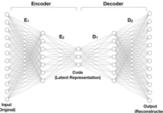
2.3 Auto-encoder
Auto-encoder is a special type of feed forward neural network for learning latent representation of the data (Figure 1). The data are fed from the input layer and encoded into a low-dimensional latent representation (code). The code is then decoded into a reconstruction of the original data. The goal of auto-encoder is to learn an identity map such that the output (reconstruction) is closely matched with the input data. The model is trained to minimize the difference between the input and the reconstruction. Auto-encoder could learn complicated nonlinear dimensionality reduction and thus is widely used in challenging tasks such as image recognition and artificial data generation.
According to universal approximation theorem [26], a feed-forward artificial neural network can approximate any continuous function given some mild assumptions about the activation functions. Theoretically, an auto-encoder with suitable activation functions could represent an identity map. Therefore, auto-encoder could learn a encoderφand decoderψsuch thatψ◦φ=I. An accurate reconstruction of the data implies a good low-dimensional representation.
Figure 1: Auto-encoder Network Architecture
3
Auto-encoding HMC
While HMC explores the parameter space more effectively, each iteration is computationally demanding since we have to evaluate a high-dimensional gradient function. To alleviate this issue, we propose a new method called Auto-encoding HMC (AE-HMC). First, we collect a small set of posterior samples from the target distribution by running the standard HMC algorithm. We then use the collected samples to find a low-dimensional latent parameter space by training an auto-encoder. Given an initial state in the original parameter space, we use the encoding part of the auto-encoder to find its projection in the latent space, simulate Hamiltonian dynamics to generate a new state, and use the decoding part of the auto-encoder to project it back to the original space to obtain a proposal. While this exploration will not be as accurate as the standard HMC, it could reduce the overall computational cost.
Illustration We illustrate our approach using a three-dimensional Gaussian distribution. Because the original dimension is very low, we use a Principle Component Analysis (PCA), which can be considered as a special case of auto-encoder [27]: the encoder of an auto-encoder reduces to a PCA if all the activation functions are linear and the inputs are normalized. Suppose we are interested in sampling from a three-dimensional Gaussian distribution with zero mean and covariance
Σ =
" 1 0.95 0.7
0.95 1 0.5 0.7 0.5 1
#
To perform dimension reduction using PCA, we simply find orthornormal matrix P such that Σ0 = PΣPT is
diagonalized, where the diagonal entries ofΣ0are the variances of the transformed variables. Here we extract the first two principal components with greatest variance as the low-dimensional representation, and simulate Hamiltonian dynamics in the latent space.
As shown in Figure 2, we only performed HMC in the space of two dimensions. But when the proposals are projected back to the original space, the algorithm still efficiently explores the space with distant proposals.
Figure 2:A:HMC trajectory in the latent space (2-dimensional); the red square is the initial position, and the blue squares are HMC proposals.B:Trajectories projected back to original parameter space (3-dimensional) showing that our method can still explore the parameter space effectively.
When it comes to high-dimensional problems, we will use auto-encoder for dimension reduction. More specifically, denote the parameters of interestqvand its latent representationqh. We also denote the encoder and decoder as
φ:qv 7→qh
ψ:qh7→qv0
whereqv0 is a reconstruction ofqv. If the error of the auto-encoder goes to zero, we have:
ψ=φ−1:qh7→qv
Our algorithm is composed of the following three stages:
1. Pre-sample a few (e.g.1000) samples ofqvusing standard HMC
2. Train an auto-encoder to fit the samples, and obtain the fitted encoderφand decoderψ
3. Run AE-HMC to proposeqv∗fromqv(a detailed version is provided in Algorithm 1):
i Findqh=φ(qv)
ii Proposeq∗hfromqhby running HMC in the latent space
iii Obtainqv∗=ψ(qh∗)
3.1 HMC in the latent space
Denote the complementary momentum ofqvaspv. The corresponding latent parameters are denoted as(qh, ph). The
auxiliary variable in the latent space is constructed using the same encoderph = φ(pv), withpv sampled from a
Gaussian distribution. Further, denote the target densityπqv(qv). We set the potential energy of the latent space to be
the negative log ofπqv(qv):
Uh(qh) =Uv(ψ(qh)) =−logπqv(ψ(qh))
Notice that this is not a re-parameterization since we will still use the potential energy function from the original space for our inference. If we use the density function ofqhinduced byφ(qv)to be the potential energy, we will need to
evaluate the volume change at each leapfrog step, which increases computational costs. As long as we could ensure detailed balance in the original space, which we will prove in later section, the MCMC proposal mechanism will be valid.
We also set the kinetic energy as follows:
Kh(ph) =Kv(ψ(ph)) =ψ(ph)TM−1ψ(ph)/2 (1)
Thus, we simulate the following Hamiltonian dynamics in the latent space:
dqhi dt = ∂Kh(ph) ∂phi dphi dt =− ∂Uh(qh) ∂qhi
The evaluation of the gradient of the potential function with respect toqh can be calculated by the chain rule. For
example, in the experiments discussed below, the decoder has one hidden layer with activation functiontanh, and the connection to the output layer is linear. We can calculate the gradient function with respect to the latent variableqhas
follows: ∂Uh(qh) ∂qh = ∂q v ∂qh T ∂U v(qv) ∂qv (2) where ∂qv ∂qh =D2diag(1−tanh2(D1qh+b1))D1 tanh(z) = e z−e−z ez+e−z, tanh 0(z) = 1−tanh2 (z)
whereD1andD2are the estimated weights of the decoder (Figure 1). A detailed calculation of the gradient ofU(qh)
regarding a logistic regression example can be found in appendix. The resulting gradient evaluation is less expensive because of the much lower dimension.
The evaluation of∂Kh(ph)
∂ph can be done in a similar way with
∂Kh(ph) ∂pv =M −1p vandpv=D2tanh(D1ph+b1), ∂Kh(ph) ∂ph ={D2diag(1−tanh2(D1ph+b1))D1}T· M−1D2tanh(D1ph+b1) (3) =D1Tdiag(1−tanh 2 (D1ph+b1))· D2TM−1D2tanh(D1ph+b1) whereDT 2M−1D2can be pre-calculated.
In practice, the Hamiltonian dynamics is simulated using leapfrog steps.
3.2 Proposal and correction
Joint distribution of(qv, pv) The density ofpvis selected to be zero-mean Gaussian with a covarianceM,
corre-sponding toKv(pv)defined in equation (1). We then have the canonical distribution of the original phase space:
πqv,pv(qv, pv)∝exp(logπqv(qv)−p
T
vM−1pv/2) (4)
Notice the induced dynamics in the phase space(qv, pv)is no longer Hamiltonian, and does not have the property
of volume preservation as standard HMC. We hereby prove that the proposed HMC update will leave the canonical distribution forqvandpv(equation 4) invariant, assuming that
i the update is time reversible and thus symmetrical
ii an appropriate volume correction term is added in the HMC acceptance probability
Time reversibility The proof is straightforward. LetTsrepresent the Hamiltonian dynamic in the latent space from
the state(qh, ph)at timetto the state(q∗h, p∗h)at timet+s. The reversibility of Hamiltonian dynamics indicates that:
Ts(q(t), p(t)) = (q(t+s), p(t+s))
Ts(q(t+s),−p(t+s)) = (q(t),−p(t))
If we letQ(q∗
h, p∗h|qh, ph)represent the process of negating momentum, applying mapping Ts and negating the
momentum again, and letΦ(qv, pv) = (φ(qv), φ(pv)),Ψ(qh, ph) = (ψ(qh), ψ(ph)), our proposal can be denoted
Q0= Ψ◦Q◦Φ. We must have:
Q0(qv∗, p∗v|qv, pv) =Q0(qv, pv|q∗v, p∗v)
A detailed proof can be found in appendix.
Detailed Balance with Volume Correction Following the proof in [28], we can show that when accounting for volume change in the acceptance ratio, detailed balance holds for our proposed Metropolis update.
Consider partitioning the phase space(q, p)into small regionsAkwith small volumeV. Suppose by applying mapping
Q0toAk, the image ofAkbecomesBk. TheBkwill also partition the space due to reversibility, but has a different
volumeV0. We need to show detailed balance:
P(Ai)T(Bj|Ai) =P(Bj)T(Ai|Bj) ∀i, j
Since wheni6=j,T(Bj|Ai) =T(Ai|Bj) = 0, we only consider wheni=j≡k:
T(Bk|Ak) =Q0(Bk|Ak) min(1,
exp(−HBk)
exp(−HAk)
V0 V )
See more details in appendix.
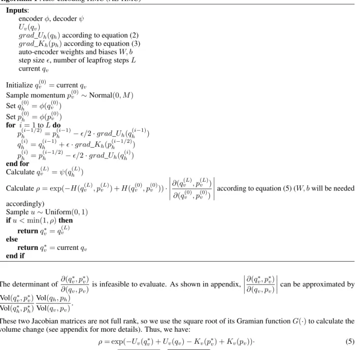
Calculation of acceptance ratio For acceptance ratioα= min(1, ρ), we have
ρ= exp(−H(q∗v, pv∗) +H(qv, pv)) ∂(qv∗, p∗v) ∂(qv, pv) = exp(−Uv(q∗v) +Uv(qv)−Kv(p∗v) +Kv(pv)) ∂(q∗v, p∗v) ∂(qv, pv)
Algorithm 1Auto-encoding HMC (AE-HMC)
Inputs:
encoderφ, decoderψ Uv(qv)
grad_Uh(qh)according to equation (2)
grad_Kh(ph)according to equation (3)
auto-encoder weights and biasesW, b
step size, number of leapfrog stepsL
currentqv
Initializeqv(0)=currentqv
Sample momentump(0)v ∼Normal(0, M)
Setqh(0)=φ(qv(0)) Setp(0)h =φ(p(0)v ) for i= 1toLdo ph(i−1/2)=ph(i−1)−/2·grad_Uh(q (i−1) h ) qh(i)=qh(i−1)+·grad_Kh(p (i−1/2) h ) ph(i)=ph(i−1/2)−/2·grad_Uh(q (i) h ) end for Calculateq(vL)=ψ(qh(L)) Calculateρ= exp(−H(q(vL), p (L) v ) +H(q (0) v , p (0) v ))· ∂(q(vL), p (L) v ) ∂(q(0)v , p (0) v )
according to equation (5) (W, bwill be needed
accordingly) Sampleu∼Uniform(0,1) ifu <min(1, ρ)then returnq∗v=q (L) v else returnq∗v=currentqv end if The determinant of ∂(q ∗ v, p∗v) ∂(qv, pv)
is infeasible to evaluate. As shown in appendix,
∂(qv∗, p∗v) ∂(qv, pv) can be approximated by Vol(q∗ v, p∗v) Vol(q∗h, p∗h) Vol(qh, ph) Vol(qv, pv) .
These two Jacobian matrices are not full rank, so we use the square root of its Gramian functionG(·)to calculate the volume change (see appendix for more details). Thus, we have:
ρ= exp(−Uv(q∗v) +Uv(qv)−Kv(p∗v) +Kv(pv))· (5) s G(∂(q ∗ v, p∗v) ∂(q∗h, p∗h)) s G(∂(qh, ph) ∂(qv, pv) ) (6)
Algorithm 1 summarizes the steps for a single iteration of AE-HMC.
3.3 Approximate Bayes inference
Given finite computational resources, in practice it would be more reasonable to keep a balance between accuracy of estimates and speed of computation. To do this, we can drop the volume adjustment. This way, instead of converging to the true distribution, our algorithm converges to an approximate but reasonably accurate distribution. In Bayesian analysis, if prediction is the ultimate goal, the resulting drop in the accuracy of estimating the posterior distribution might not lead to substantial deterioration in the prediction accuracy. Note that our method would still be preferable to those that only provide point estimates for predictions since it provides a reasonable estimate of prediction uncertainty.
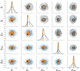
Illustration To demonstrate that the approximate posterior distribution provided by AE-HMC can still capture high probability regions, we conduct a high-dimensional logistic regression experiment with simulated data.
Figure 3: Comparing posterior distributions based on Standard HMC (blue) and Auto-encoding HMC (orange). As we can see, although the approximate distributions provided by AE-HMC tend to be more concentrated, they clearly cover the true parameter values (black).
In this experiment, we create a relatively challenging synthetic dataset for binary classification with 500 features from which 50 of them are highly correlated (ρ= 0.85), and the rest are sampled from a standard normal distribution. In total, we simulate 550 data points for training and 150 for testing. We assumeβ’s haveN(0,102)priors.
We first run the standard HMC to obtain 1000 samples, which are used to train the auto-encoder. For both standard HMC and AE-HMC, we tune the acceptance rate to be around 0.65 to 0.7, which is optimal in terms of computational efficiency [29]. We compare the results using1000samples after the convergence has been reached.
Figure 3 shows the posterior distributions of five differentβ’s for both sampling methods. As we can see, our method still provides a reasonable approximation of the posterior distribution (at much lower computational cost as shown in the next section). Similar results are obtained for other parameters.
4
Experiments
In this section, we evaluate the performance of our proposed method by comparing it to standard HMC. To this end, we will use two types of models: 1) high dimensional Bayesian logistic regression, and 2) high dimensional Bayesian inverse problem with Eliptic PDE.
4.1 High-dimensional Bayesian logistic regression
Along with the synthetic dataset discussed above, we also examine our method based on three real datasets: CNAE-9, Optical Recognition of Handwritten Digits (both from the UCI Machine Learning Repository), and MNIST. For each dataset, we only focus on the first two groups for binary classification.
We use STAN [30] and Keras [31] with the TensorFlow backend to implement our method and compare its performance to the standard HMC algorithm implemented in STAN.
We use an auto-encoder of three fully connected layers with linear activation where the dimension of the middle layer is roughly ten times smaller than the input layer. In the first step, we generate initial samples (from the warm-up stage) for training the auto-encoder using STAN. These samples consisted of approximately 10% of the full HMC simulation. Then the auto-encoder is trained using these samples and its weights are extracted for custom implementation in STAN in order to generate samples from the latent space. Then, the samples are projected back to the original space followed by the accept-reject step.
As we can see in Table 1, our method could substantially improve the speed of Bayesian inference, while providing accuracy rates similar to those of standard HMC.
Method Dataset Synthetic CNAE9 Digits MNIST #Parameters 500 856 64 784 HMC Time 11,077.8 3,793.3 865.7 33,300.8 Accuracy 82% 98.3% 100% 99.6% #Parameters 50 85 6 78 AE-HMC Time 3,471.8 1,083.0 145.6 4,878.5 Accuracy 82% 98.3% 100% 99.2% Speed-up 3.2 3.5 5.9 6.8
Table 1: Comparing accuracy rate (on test sets) and computational cost (time in second) of HMC and AE-HMC based on four different logisitic regression models. The number of parameters for AE-HMC shows the dimension of the latent space. Both methods use the same number of MCMC iterations.
4.2 High-dimensional Bayesian inverse problem with elliptic PDE
Next, we examine the performance of our method using a more complex model — Bayesian inverse problem. The model involves the following elliptic PDE defined on the unit square domainΩ = [0,1]2:
−∇ ·(k(s)∇p(s)) =f(s), s∈Ω hk(s)∇p(s), ~n(s)i= 0, s∈∂Ω
Z
∂Ω
p(s)dl(s) = 0
wherek(s)is the transmissivity field,p(s)is the potential function,f(s)is the forcing term, and~n(s)is the outward normal to the boundary.
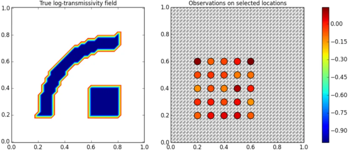
To generate data, we construct a true transmissivity fieldk0(s)as shown on the left panel of the Figure 4. Partial
observations are obtained by solvingp(s)on an80×80mesh and then collecting at25measurement sensors as shown by the circles on the right panel of the Figure 4. The corresponding observation operatorOyields the data
y=Op(s) +η, η ∼ N(0, ση2I25)
where the signal-to-noise ratio is set at SNR:= maxs{u(s)}/ση = 10.
The inverse problem involves finding the transmissivity fieldk(s)from the observations. Bayesian approach endows a log-Gaussian prior fork(s):
k(s) = exp(u(s)), u(s)∼ N(0,C)
Figure 4: True log-transmissivity fieldu0(s)(left), and25observations on selected locations indicated by circles (right),
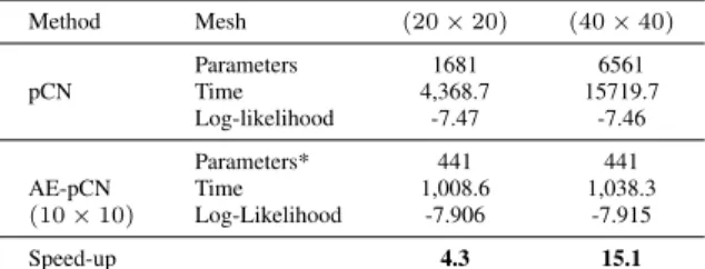
Method Mesh (20×20) (40×40) Parameters 1681 6561 pCN Time 4,368.7 15719.7 Log-likelihood -7.47 -7.46 Parameters* 441 441 AE-pCN Time 1,008.6 1,038.3 (10×10) Log-Likelihood -7.906 -7.915 Speed-up 4.3 15.1
Table 2: Comparing accuracy (in terms of log-likelihood) and computational cost (time in second) of pCN and AE-pCN based on a high dimensional Bayesian inverse problem involving Eliptic PDE. The number of parameters for AE-HMC shows the dimension of the latent space. Both methods use the same number of MCMC iterations.
where the covariance operatorCis defined through an exponential kernel function C:X→X, u(s)7→ Z c(s, s0)u(s0)ds0, c(s, s0) =σu2exp −ks−s 0k 2s0 ,fors, s0∈Ω
with the prior standard deviationσu = 1.25and the correlation lengths0 = 0.0625in the experiment. Then, the
problem reduces to sampling from the posterior of the log-transmissivity fieldu(s), which becomes a vector of dimension over6500after being discretized on40×40mesh (with Lagrange degree2). See more details in [32, 33] This is a very challenging sampling problem. To make the sampling rigorous in such a high dimensional space, we refer to the following pre-conditioned Crank-Nicolson (pCN) proposal, which can be viewed as a variant of RWM [34, 33]:
qv∗=ρ qv+ p 1−ρ2p v, pv∼ N(0,C) whereρ= (1−h 4)/(1 + h
4)withhbeing the step size. We follow the same procedure as AE-HMC to projectqvtoqh
in the latent space of a much smaller dimension e.g. 600, make a proposalq∗
hbased on the above proposal and finally
map it back the original space. We refer to this modified version of our method as AE-pCN.
We run pCN on two mesh sizes(20×20)and(40×40)which are reduced to a problem of size(10×10)using AE-pCN. We observe on Table 2 a significant reduction on computation time but similar log-likelihood values using our proposed method. These results indicate an excellent trade-off between computational run time and the log-likelihood approximation.
5
Discussion
In this paper, we have proposed a new approach for approximating high dimensional probability distributions for fast, yet accurate Bayesian inference. Using synthetic and real data, we have shown that the resulting algorithm achieves a good balance between computational cost and posterior approximation.
There are some possible future directions worth pursuing. First, our method loses a nice property of standard HMC, namely, volume preservation. If a volume preserving embedding can be developed, it will allow for better approximation of posterior distribution.
The computational saving mainly depends on the dimension of the latent space. However, reducing dimension empirically could lead to substantial loss of information. More work needs to be done to automatically determine the optimal size of the latent space. In addition, it is conceivable that some specific auto-encoder architectures and activation functions could provide better trade-offs between computational cost and accuracy.
Finally, note that our work can be extended to other MCMC algorithms using a similar framework (as shown in the previous section). Also, because our method focuses on high-dimensional problems with a large number of parameters, conceptually, it can be combined with some recent sampling algorithms that focus on problems with large sample sizes.
Acknowledgement
Appendix
A
Calculating the gradient of
U
h(
q
h)
for Bayesian logistic regression
Consider a logistic regression model yi|Xi, qv ∼ Bern(πi), πi = 1+exp(1−X
iqv), where Xi =
(Xi1, Xi2,· · ·, XiD), qv= (qv1, qv2,· · · , qvD)T. We set the prior to be zero mean Gaussian with unit variance.
The total Likelihood isp(y|X, qv) = N Q i=1 1 1 + exp(−Xiqv) yi 1 1 + exp(Xiqv) 1−yi
Given that the decoder has one hidden layer andtanhis used as the activation function, we have:
qv=D2tanh(D1qh+b1). Consider Uv(qv) =−log(p(qv))−logp(y|X, qv) = 1 2q T vqv− N X i=1 yilog 1 1 + exp(−Xiqv) + (1−yi) log 1 1 + exp(Xiqv) = 1 2q T vqv− N X i=1 yi(Xiqv) + N X i=1 log(1 + exp(Xiqv)) ∂Uv(qv) ∂qv =qv−XTD×N y− 1 1 + exp(−Xqv) N×1 =qv− N X i=1 XTiyi+ N X i=1 XT i 1 + exp(−Xiqv) Thus, ∂Uh(qh) ∂qh =∂Uv(qv) ∂qh = ∂q v ∂qh T ∂U v(qv) ∂qv = D2diag(1−tanh2(D1qh+b1))D1 T · D2tanh(D1qh+b1)−XTy+XT 1 1 + exp(−XD2tanh(D1qh+b1)) =D1Tdiag(1−tanh2(D1ph+b1))· " DT2D2tanh(D1qh+b1)− N X i=1 (XiD2)Tyi+ N X i=1 (XiD2)T 1 + exp(−XiD2tanh(D1qh+b1)) # (7) whereDT
2D2andXiD2can be pre-calculated. Notice that dim(XiD2)<<dim(Xi).
B
Time reversibility
Given thatψis the inverse map ofφ, and define functionh(q, p) = (q,−p)we have Ψ(Q(Φ(qv, pv))) = Ψ(Q(φ(qv), φ(pv))) = Ψ(Q(qh, ph)) = Ψ(h◦Ts◦h(qh, ph)) = Ψ(h◦Ts(qh,−ph)) = Ψ(h(q∗h,−p∗h)) = Ψ(qh∗, p∗h) = (ψ(q∗h), ψ(p∗h)) = (q∗v, p∗v)
and Ψ(Q(Φ(qv∗, p∗v))) = Ψ(Q(Ψ−1(qv∗, p∗v))) = Ψ(Q(ψ−1(qv∗), ψ− 1 (p∗v))) = Ψ(Q(q∗h, p∗h)) = Ψ(h◦Ts◦h(q∗h, p∗h)) = Ψ(h◦Ts(qh∗,−p ∗ h)) = Ψ(h(qh,−ph)) = Ψ(qh, ph) = Φ−1(qh, ph) = (φ−1(qh), φ−1(ph)) = (qv, pv) ThusQ0= Ψ◦Q◦Φis symmetric.
C
Detailed Balance with Volume Correction
Following the proof in [28], we can show that when accounting for volume change in the acceptance ratio, detailed balance holds for our proposed Metropolis update.
Consider partitioning the phase space(q, p)into small regionsAkwith small volumeV. Suppose by applying mapping
Q0toAk, the image ofAkbecomesBk. TheBkwill also partition the space due to reversibility, but has a different
volumeV0. We need to show detailed balance:
P(Ai)T(Bj|Ai) =P(Bj)T(Ai|Bj) ∀i, j
Since wheni6=j,T(Bj|Ai) =T(Ai|Bj) = 0, we only consider wheni=j≡k. Let
T(Bk|Ak) =Q0(Bk|Ak) min(1,
exp(−HBk)
exp(−HAk)
V0 V )
Then, we can writeP(Ak)T(Bk|Ak)as
Vexp(−HAk)Q 0(B k|Ak) min(1, exp(−HBk) exp(−HAk) V0 V ) =Q0(Bk|Ak) min(V exp(−HAk), V 0exp(−H Bk)) =Q0(Ak|Bk) min(V exp(−HAk), V 0exp(−H Bk)) =V0exp(−HBk)Q 0(B k|Ak) min( exp(−HAk) exp(−HBk) V V0,1) =P(Bk)T(Ak|Bk)
The volume correction termV
0
V is simply the determinant of the Jacobian matrix
∂(qv∗, p∗v) ∂(qv, pv) .
D
Approximating volume correction term
Following [28], let’s consider a one dimensional example. For mapping
Tδ(q, p) = q p +δ dq/dt dp/dt +O(δ2)
The Jacobian matrix:
Bδ = 1 +δ∂ 2H ∂q∂p δ ∂2H ∂p2 −δ∂ 2H ∂q2 1−δ ∂2H ∂p∂q +O(δ2)
Consider a3×2matrix A and2×3matrix C: "a 11 a12 a21 a22 a31 a32 # 1 +δ∂ 2H ∂q∂p δ ∂2H ∂p2 −δ∂ 2H ∂q2 1−δ ∂2H ∂p∂q +O(δ2) c11 c12 c13 c21 c22 c23
It gives a3×3matrix with element(i, j)to be
ai1c1j+ai2c2j+δ(ai1c1j ∂2H ∂q∂p−ai2c1j ∂2H ∂p2 +ai1c2j ∂2H ∂p2 −ai2c2j ∂2H ∂p∂q) +O(δ 2)
We could show that
det(ABδC) = det(AC) +O(δ2)
The result can be generalized to higher dimensions. Now let’s denotez= (q, p),Ai=
∂zi v ∂zi h ,Bδ= ∂zi h ∂zih−1,Ci = ∂zi h ∂zi v . We have: det(∂z L v ∂z0 v ) = det(∂z L v ∂zL h ∂zL h ∂zLh−1 ∂zLh−1 ∂zLv−1 · · ·∂z 1 v ∂z1 h ∂z1 h ∂z0 h ∂z0 h ∂z0 v ) = det(ALBδCL−1AL−1· · ·A1BδC0)
= det(ALBδCL−1) det(AL−1BδCL−2)· · ·det(A1BδC0)
= (det(ALCL−1) +O(δ2))(det(AL−1CL−2) +O(δ2))· · ·(det(A1C0) +O(δ2))
=V ol(z L v) V ol(zL h) V ol(z0 h) V ol(z0 v) +O(δ) → V ol(z L v) V ol(zL h) V ol(z0 h) V ol(z0 v) asδ→0
For matricesALandC0, the number of vectors are less than the dimension of the ambient space. We could use the square
root of the gramian function of the matrix to calculatek-volume inn-space wherek < n. In particular, forklinearly independent vectorsv1,· · · , vk, the gramian function isG(v1, ..., vk) =det(MTM)whereM = (v1,· · ·, vk). The
volume of the parallelepiped with the vectors is calculated by:
V ol(v1, ..., vk) =
q
det(MTM)
References
[1] B. Shahbaba, S. Lan, W.O. Johnson, and R.M. Neal. Split Hamiltonian Monte Carlo. Statistics and Computing, 24(3):339–349, 2014.
[2] M. Welling and Y. W. Teh. Bayesian learning via stochastic gradient Langevin dynamics. InProceedings of the
International Conference on Machine Learning, 2011.
[3] M. Hoffman and A. Gelman. The No-U-Turn Sampler: Adaptively Setting Path Lengths in Hamiltonian Monte Carlo. arxiv.org/abs/1111.4246, 2011.
[4] S. Lan, B. Zhou, and B. Shahbaba. Spherical Hamiltonian Monte Carlo for constrained target distributions. In
Proceedings of the 31th International Conference on Machine Learning (ICML), (2014).
[5] S. Lan, J. Streets, and B. Shahbaba. Wormhole hamiltonian monte carlo. InProceedings of the Twenty-Eighth
AAAI Conference on Artificial Intelligence, 2014.
[6] Matthew D. Hoffman, David M. Blei, and Francis R. Bach. Online learning for latent dirichlet allocation. In John D. Lafferty, Christopher K. I. Williams, John Shawe-Taylor, Richard S. Zemel, and Aron Culotta, editors,
NIPS, pages 856–864. Curran Associates, Inc., 2010.
[8] Michael Betancourt. The fundamental incompatibility of scalable hamiltonian monte carlo and naive data subsampling. InProceedings of the 32nd International Conference on Machine Learning, ICML 2015, Lille,
France, 6-11 July 2015, pages 533–540, 2015.
[9] Heiko Strathmann, Dino Sejdinovic, Samuel Livingstone, Zoltan Szabo, and Arthur Gretton. Gradient-free hamiltonian monte carlo with efficient kernel exponential families. InProceedings of the 28th International
Conference on Neural Information Processing Systems - Volume 1, NIPS’15, pages 955–963, Cambridge, MA,
USA, 2015. MIT Press.
[10] C. Zhang, B. Shahbaba, and H. Zhao. Precomputing strategy for Hamiltonian Monte Carlo method based on regularity in parameter space. Computational Statistics, 32(1), 2017.
[11] C. Zhang, B. Shahbaba, and H. Zhao. Hamiltonian Monte Carlo acceleration using surrogate functions with random bases. Statistics and Computing, 27(6), 2017.
[12] Jiaming Song, Shengjia Zhao, and Stefano Ermon. A-nice-mc: Adversarial training for mcmc. In I. Guyon, U. V. Luxburg, S. Bengio, H. Wallach, R. Fergus, S. Vishwanathan, and R. Garnett, editors,Advances in Neural
Information Processing Systems 30, pages 5140–5150. Curran Associates, Inc., 2017.
[13] Daniel Levy, Matthew D. Hoffman, and Jascha Sohl-Dickstein. Generalizing hamiltonian monte carlo with neural networks, 2017.
[14] Lingge Li, Andrew Holbrook, Babak Shahbaba, and Pierre Baldi. Neural Network Gradient Hamiltonian Monte Carlo. Computational Statistics, 34(1):281–299, 2019.
[15] M. I. Jordan, Z. Ghahramani, T. S. Jaakkola, and L. K. Saul. An introduction to variational methods for graphical methods. InMachine Learning, pages 183–233. MIT Press, 1999.
[16] M. Wainwright and M. Jordan. Graphical models, exponential families, and variational inference.Foundations
and Trends in Machine Learning, 1(1-2):1–305, 2008.
[17] A. Honkela, T. Raiko, M. Kuusela, M. Tornio, and J. Karhunen. Approximate Riemannian conjugate gradient learning for fixed-form variational Bayes. Journal of Machine Learning Research, 11:3235–3268, 2010. [18] L. Saul and M. I. Jordan. Exploiting tractable substructures in intractable networks. In G. Tesauro, D. S. Touretzky,
and T. K. Leen, editors, Advance in neural information processing systems 7 (NIPS 1996), pages 486–492, Cambridge, MA, 1996. MIT Press.
[19] T. Salimans and D. A. Knowles. Fixed-form variational posterior approximation through stochastic linear regression. Bayesian Analysis, 8(4):837–882, 2013.
[20] N. de Freitas, P. Højen-Sørensen, M. Jordan, and R. Stuart. Variational MCMC. InProceedings of the 17th
Conference in Uncertainty in Artificial Intelligence, UAI ’01, pages 120–127, San Francisco, CA, USA, 2001.
Morgan Kaufmann Publishers Inc.
[21] Tim Salimans, Diederik Kingma, and Max Welling. Markov chain monte carlo and variational inference: Bridging the gap. In Francis Bach and David Blei, editors,Proceedings of the 32nd International Conference on Machine
Learning, volume 37, pages 1218–1226. PMLR, 2015.
[22] C. Zhang, B. Shahbaba, and H. Zhao. Variational hamiltonian Monte Carlo via score matching.Bayesian Analysis, 13(2), 2018.
[23] Michael Betancourt. A conceptual introduction to hamiltonian monte carlo.arXiv preprint arXiv:1701.02434, 2017.
[24] S. Duane, A. D. Kennedy, B J. Pendleton, and D. Roweth. Hybrid Monte Carlo. Physics Letters B, 195(2):216 – 222, 1987.
[25] R.M. Neal. MCMC using Hamiltonian dynamics. In S. Brooks, A. Gelman, G. Jones, and X. L. Meng, editors,
Handbook of Markov Chain Monte Carlo, pages 113–162. Chapman and Hall/CRC, 2011.
[26] Balázs Csanád Csáji. Approximation with artificial neural networks.Faculty of Sciences, Etvs Lornd University,
Hungary, 24:48, 2001.
[27] P. Baldi and K. Hornik. Neural networks and principal component analysis: Learning from examples without local minima. Neural Netw., 2(1):53–58, January 1989.
[28] Radford M Neal et al. Mcmc using hamiltonian dynamics. Handbook of Markov Chain Monte Carlo, 2(11):2, 2011.
[29] Alexandros Beskos, Natesh Pillai, Gareth Roberts, Jesus-Maria Sanz-Serna, Andrew Stuart, et al. Optimal tuning of the hybrid monte carlo algorithm. Bernoulli, 19(5A):1501–1534, 2013.
[30] Stan Development Team. Pystan: the python interface to stan, version 2.17.1.0.http://mc-stan.org, 2018. [31] François Chollet et al. Keras.https://keras.io, 2015.
[32] Tiangang Cui, Kody J.H. Law, and Youssef M. Marzouk. Dimension-independent likelihood-informed MCMC.
Journal of Computational Physics, 304:109 – 137, 2016.
[33] Shiwei Lan. Adaptive dimension reduction to accelerate infinite-dimensional geometric markov chain monte carlo.
Journal of Computational Physics, 392:71 – 95, 2019.
[34] Alexandros Beskos, Mark Girolami, Shiwei Lan, Patrick E. Farrell, and Andrew M. Stuart. Geometric mcmc for infinite-dimensional inverse problems.Journal of Computational Physics, 335:327 – 351, 2017.