TI 2011-004/4
Tinbergen Institute Discussion Paper
A Class of Adaptive EM-based
Importance Sampling Algorithms for
Efficient and Robust Posterior and
Predictive Simulation
Lennart Hoogerheide
Anne Opschoor
Herman K. van Dijk
Tinbergen Institute is the graduate school and research institute in economics of Erasmus University Rotterdam, the University of Amsterdam and VU University Amsterdam. More TI discussion papers can be downloaded at http://www.tinbergen.nl
Tinbergen Institute has two locations: Tinbergen Institute Amsterdam Gustav Mahlerplein 117 1082 MS Amsterdam The Netherlands Tel.: +31(0)20 525 1600 Tinbergen Institute Rotterdam Burg. Oudlaan 50
3062 PA Rotterdam The Netherlands Tel.: +31(0)10 408 8900 Fax: +31(0)10 408 9031
Duisenberg school of finance is a collaboration of the Dutch financial sector and universities, with the ambition to support innovative research and offer top quality academic education in core areas of finance.
DSF research papers can be downloaded at: http://www.dsf.nl/
Duisenberg school of finance Gustav Mahlerplein 117 1082 MS Amsterdam The Netherlands Tel.: +31(0)20 525 8579
A Class of Adaptive EM-based Importance Sampling Algorithms
for Efficient and Robust Posterior and Predictive Simulation
Lennart Hoogerheide
∗†Anne Opschoor
∗Herman K. van Dijk
∗Abstract
A class of adaptive sampling methods is introduced for efficient posterior and predictive simulation. The proposed methods are robust in the sense that they can handle target dis-tributions that exhibit non-elliptical shapes such as multimodality and skewness. The basic method makes use of sequences of importance weighted Expectation Maximization steps in order to efficiently construct a mixture of Student-tdensities that approximates accurately the target distribution – typically a posterior distribution, of which we only require a kernel – in the sense that the Kullback-Leibler divergence between target and mixture is minimized. We label this approachMixture of t by Importance Sampling and Expectation Maximization
(MitISEM). The constructed mixture is used as a candidate density for quick and reliable application of either Importance Sampling (IS) or the Metropolis-Hastings (MH) method. The MitISEM algorithm performs well in exploring non-elliptical shapes of posterior and predictive distributions, in estimating predictive likelihoods and forecasting Value at Risk, for several examples of statistical and econometric models. We also introduce three exten-sions of the basic MitISEM approach. First, we propose a method for applying MitISEM in a sequential manner, so that the candidate distribution for posterior simulation is cleverly updated when new data become available. Our results show that the computational ef-fort reduces enormously, while the quality of the approximation remains almost unchanged. This sequential approach can be combined with a tempering approach, which facilitates the simulation from densities with multiple modes that are far apart. Second, we introduce a
permutation-augmented MitISEM approach, for importance sampling from posterior distri-butions in mixture models without the requirement of imposing identification restrictions on the model’s mixture regimes’ parameters. Third, we propose a partial MitISEM approach, which aims at approximating the marginal and conditional posterior distributions of sub-sets of model parameters, rather than the joint. This division can substantially reduce the dimension of the approximation problem, which facilitates the application of adaptive im-portance sampling for posterior simulation in more complex models with larger numbers of parameters. Our results indicate that the proposed methods can substantially reduce the computational burden in econometric models like mixture GARCH models and a mixture instrumental variables model.
∗Econometric and Tinbergen Institutes, Erasmus University Rotterdam, The Netherlands †Corresponding author, e-mail address: [email protected].
Keywords: mixture of Student-tdistributions, importance sampling, Kullback-Leibler di-vergence, Expectation Maximization, Metropolis-Hastings algorithm, predictive likelihoods, Mixture GARCH models, Value at Risk.
1
Introduction
Since a few decades there is considerable interest in Bayesian analysis using computer gen-erated pseudo random draws from the posterior and predictive distribution. Markov Chain Monte Carlo (MCMC) techniques are useful for this purpose and a popular MCMC technique is the Metropolis-Hastings algorithm, developed by Metropolis et al. (1953) and generalized by Hastings (1970). Several updates of this sampler are proposed in the literature, especially the idea of adapting the proposal distribution given sampled draws.
Monte Carlo procedures based on Importance Sampling (IS), see Hammersley and Hand-scomb (1964), are an alternative. This idea has been introduced in Bayesian inference by Kloek and Van Dijk (1978) and is further developed by Van Dijk and Kloek (1980, 1984)
and, in particular, by Geweke (1989). According to Capp´e et al. (2008), there exists
re-newed interest in Importance Sampling. This is due to its relatively simple properties which allow for the development of parallel implementation. The increased popularity of Impor-tance Sampling goes jointly with the development of multiple core machines and computer clusters.
In this paper we specify a class of adaptive sampling methods for efficient and reliable posterior and predictive simulation. The proposed methods are robust in the sense that they can handle target distributions that exhibit non-elliptical shapes such as multimodal-ity and skewness. These methods are especially useful for posteriors where the convergence of alternative simulation methods is slow or even doubtful, such as high serial correlation in Gibbs sequences that may be caused by large numbers of latent variables or non-elliptical shapes. Importance Sampling and Gibbs sampling are not necessarily substitutes: given that diagnostic checks can never fully guarantee that results have converged to the true values (that is, that convergence has been reached and that no errors have been made in the derivations and code), the use of both simulation methods that have completely different theory and implementation can be a useful validity check. Further, an appropriate candi-date distribution can be used to draw initial values for multiple Gibbs sequences, whereas a sample of Gibbs draws can be used to obtain initial values for the mean and covariance matrix in the process of constructing an approximating candidate distribution. Our
pro-posed methods make use of the novel Mixture of t by Importance Sampling and Expectation
steps in an Expectation Maximization algorithm in order to relatively quickly construct a
mixture of Student-t densities, which is used as an efficient and reliable candidate density
for Importance Sampling (IS) or the Metropolis-Hastings (MH) method. Next to assessing possibly non-elliptical posterior distributions, MitISEM is particulary useful for accurately estimating marginal and predictive likelihoods via IS.
Apart from specifying the basic approach of MitISEM, we introduce three extensions. First, we propose a method for applying MitISEM in a sequential manner, so that the candidate distribution for posterior simulation is cleverly updated when new data become available. Our results show that the computational effort reduces enormously, while the quality of the approximation remains almost unchanged, as compared with an ‘ad hoc’ procedure in which the construction of the MitISEM candidate is performed ‘from scratch’ at every moment in time. This sequential approach can be combined with a tempering approach, which facilitates the simulation from densities with multiple modes that are far apart. The proposed tempering method moves sequentially from a tempered target density kernel, the target density kernel to the power of a positive number that is smaller than 1, towards the real target density kernel. The tempered target distribution is more diffuse and hence the probability of detecting far-away modes is higher. This tempering idea is used in the Equi-Energy sampler, developed by Kou, Zhou and Wong (2006).
Second, we introduce a permutation-augmented MitISEM approach, for importance sam-pling from posterior distributions in mixture models without the requirement of imposing
a priori identification restrictions on the mixture components’ parameters. As discussed by Geweke (2007), the mixture model likelihood function is invariant with respect to per-mutation of the components of the mixture model. If functions of interest are perper-mutation sensitive, as in classification applications, then interpretation of the likelihood function re-quires valid inequality constraints. If functions of interest are permutation invariant, as in prediction applications, then there are no such problems of interpretation. Geweke (2007) proposes the permutation-augmented Gibbs sampler, which can be considered as an
exten-sion of the random permutation sampler of Fr¨uhwirth-Schnatter (2001). The practical
im-plementation of the idea of the permutation-augmented Gibbs sampler is that one simulates a Gibbs sequence with total disregard for label switching or the prior’s labeling restrictions. Only after that and only if functions of interest are permutation sensitive, then one simply permutes the Gibbs sampler’s output so as to satisfy the labeling restrictions. We propose a method of permutation-augmented IS, for which we extend the MitISEM approach to con-struct an approximation to the unrestricted posterior, taking into account the permutation
Student-t component to the candidate implies an addition of the m! equivalent
permuta-tions. Thereby, we construct a mixture of mixtures ofm! Student-t components, where the
restriction is imposed that the m! permutations have equal candidate density. Intuitively
stated, we help the basic MitISEM approach by ‘telling’ it about the invariance with respect to permutations. It should be noted that this invariance with respect to permutations is not the only possible cause of non-elliptical shapes in a mixture model’s posterior. For example, if the probability of one of the model’s components tends to zero, the local non-identification of the component’s other parameters causes ridge shapes.
Third, we propose a partial MitISEM approach, which aims at approximating the marginal and conditional posterior distributions of subsets of model parameters, rather than the joint. This division can substantially reduce the dimension of the approximation problem, which facilitates the application of adaptive importance sampling for posterior simulation in more complex models with larger numbers of parameters. Approximating the
joint posterior density kernel with a mixture of Student-tdistributions allows for a huge
flex-ibility of shapes. However, rarely all of this flexflex-ibility is required. It is typically enough to
use mixtures of Student-tdistributions for the dependencewithin subsets of the parameters.
We can often divide the parameters into subsets, where the dependence between different
subsets is less complicated. Our partial MitISEM approach divides the model parameters into ordered subsets, where the conditional candidate distributions’ means are linear com-binations of (functions of) the parameters in previous subsets. The conditional candidate distributions’ covariances can also be made to depend on the parameters in previous sub-sets, by allowing the probabilities of the mixture components of the conditional candidate distribution to differ for different ranges of values for functions of the parameters in pre-vious subsets. The partial MitISEM approach is a way to provide a usable approximation to the posterior, while preventing problems such as numerical issues with specifying huge covariance matrices for a joint candidate distribution – problems that have led researchers to conclude that IS necessarily suffers from a ‘curse of dimensionality’.
Several approaches of adaptive sampling using mixtures exist in the literature. Keith et al. (2008) developed adaptive independence samplers by minimizing the Kullback-Leibler (KL) divergence in order to provide the best candidate density, which consists of a mix-ture of Gaussian densities. The minimization of the KL-divergence is done by applying the EM algorithm of Dempster et al. (1977) and the number of mixture components is selected through information criteria like AIC (Akaike (1974)), BIC (Schwarz (1978)) or DIC (Gel-man et al. (2003)). Our basic approach is a ‘bottom up’ procedure that starts with one
added iteratively until a certain stop criterion is met. We emphasize that the IS-weighted version of the EM algorithm is applied in order to use all candidate draws without requiring the Metropolis-Hastings algorithm to transform the candidate draws into a set of posterior draws. The advantages are that we do not require a burn-in sample, that the use of all candidate draws helps to prevent numerical problems with estimating candidate covariance matrices – also draws with relatively small, but positive importance weights are helpful for this purpose – and that the use of all candidate draws may lead to a better approximation.
Capp´e et al. (2008) and Cornuet et al. (2009) also use IS-weights in the EM algorithm with
a mixture of Student-t densities as candidate density. Capp´e et al. (2008) developed the
M-PMC (Mixture Population Monte Carlo) algorithm, which is an adaptive algorithm that iteratively updates both the weights and component parameters of a mixture importance
sampling density. An important difference between Capp´e et al. (2008) (and also Cornuet
et al. (2009)) and the present paper is the choice of the number of mixture components and
the starting values of the candidate mixture’s Student-tcomponents’ means and covariances
in the EM optimization procedure. Regarding the first issue, in earlier papers the number of mixture components is chosen a priori, where we let the algorithm choose the required number of components. Second, we choose the starting values based on the draws that
correspond to the highest IS-weights for the previous mixture of Student-t candidate in the
algorithm, where Capp´e et al. (2008) do not provide a strategy for choosing starting values.
Although the EM procedure is guaranteed to converge to a local optimum, the choice of
the starting values may still be crucial, given that the KL divergence between target and candidate (as a function of the candidate mixture’s means, covariances, degrees of freedom and component weights) is a highly non-elliptical, multimodal function. Moreover, we pro-vide extensions (sequential, tempered, permutation-augmented and partial MitISEM) that facilitate simulation for specific applications and for particular statistical and econometric models.
A final remark considering the literature regards the Adaptive Mixture of t (AdMit) approach of Hoogerheide, Kaashoek and Van Dijk (2007). Whereas the idea behind AdMit and MitISEM is the same, i.e. iteratively constructing an approximation of a target
distri-bution by a mixture of Student-tdistributions, there are three substantial differences. First,
AdMit aims at minimizing the variance of the IS estimator directly, whereas MitISEM aims at this goal indirectly by minimizing the Kullback-Leibler divergence. As a result, AdMit optimizes the mixture component weights using a non-linear optimization procedure that requires considerable computational effort. Second, in the AdMit method, means and covari-ance matrices of the candidate components are chosen heuristically and are never updated
when additional components are added to the mixture, whereas in MitISEM all mixture pa-rameters are optimized jointly by means of the relatively quick EM algorithm. This implies a large reduction of the computing time in the approximation procedure, and is expected to lead to a better candidate in most applications. Third, AdMit requires the joint target density kernel, whereas MitISEM requires candidate draws and importance weights. This implies that AdMit can not be applied partially to the marginal and conditional posterior distributions of subsets of parameters, whereas we propose a partial MitISEM approach. One relative advantage of the AdMit approach is the step in which the importance weight function is maximized with respect to the parameter vector, which may lead to finding relevant areas of the parameter space that were ‘missed’ by all draws from the previous candidate. We intend to investigate the use of such an AdMit step within MitISEM in further research.
The outline of this paper is as follows. In section 2 we introduce the MitISEM method. Section 2 also provides three subsections of applications in which MitISEM is used for estimating posterior moments, forecasting Value at Risk, and estimating model probabilities. Section 3 introduces the sequential MitISEM method, and includes a subsection on the tempering method. Section 4 introduces the partial MitISEM method. Section 5 concludes. The appendix provides the derivations of the IS-weighted EM methods.
2
Mixture of t by Importance Sampling and
Expecta-tion MaximizaExpecta-tion (MitISEM)
If one uses Importance Sampling or the Metropolis-Hastings algorithm to conduct posterior analysis, a key issue is to find a candidate density which approximates the target distribu-tion. This can be quite difficult if the target density is not elliptical. This paper proposes
to specify the candidate distribution as a mixture of Student-t distributions. According
to Hoogerheide et al. (2007), the usage of mixtures of Student-t distributions has several
advantages. First, they can provide an accurate approximation to a wide variety of target densities. For example, they can exhibit substantial skewness or irregularly curved contours such as multimodality. Zeevi and Meir (1997) show that under certain conditions any den-sity function may be approximated to arbitrary accuracy by a convex combination of ‘basis’
densities; the mixture of Student-tdensities falls within their framework. Second, simulation
from the Student-t distribution and evaluation of the Student-t density are performed easily
and efficiently. Third, Student-t distributions have fatter tails than normal distributions,
target distribution. Fourth, a mixture of t approximation to a target distribution can be constructed in a quick, automatic, reliable manner by our novel procedure.
We will use the notationf(θ) for the target density kernel of θ, the k-dimensional vector
of interest. f(θ) is typically a posterior density kernel, but it can also be a density kernel of
observable variables or a density kernel of both parameters and observable variables. g(θ)
is the candidate density, a mixture ofH Student-t densities:
g(θ) =g(θ|ζ) =
H
∑
h=1
ηh tk(θ|µh,Σh, νh), (1)
where ζ is the set of modes µh, scale matrices Σh, degrees of freedom νh, and mixing
probabilitiesηh (h= 1, . . . , H) of the k-dimensional Student-t components with density:
tk(θ|µh,Σh, νh) = Γ(νh+k 2 ) Γ(νh 2 ) (πνh)k/2 |Σh|−1/2 ( 1 + (θ−µh) ′ Σ−h1(θ−µh) νh )−(k+νh)/2 . (2)
Here Σh is positive definite, ηh ≥ 0 and
∑H
h=1ηh = 1. We further restrict νh such that
νh ≥1.
First, assume that the number of components H is given. In the sequel of this section
we will propose a ‘bottom up’ procedure that starts with one Student-t distribution and
which iteratively adds Student-t components until a certain stop criterion is met. The
aim is to choose the candidate mixture density g(θ) in such a way that it provides a good
approximation of the target density ˜f(θ) of whichf(θ) is a kernel. We do this by choosingζ
such that it minimizes the Kullback-Leibler divergence (or Cross-entropy distance) (Kullback and Leibler (1951)), which is defined as
D1( ˜f →g) =
∫
˜
f(θ) log f˜(θ)
g(θ|ζ) dθ. (3) This is obviously equivalent with minimizing
D1(f →g) =
∫
f(θ) log f(θ)
g(θ|ζ) dθ. (4)
as long as the same kernel f of the target density ˜f is used throughout the minimization.
Since D1(f →g) = ∫ f(θ) log f(θ) g(θ|ζ) dθ = ∫ f(θ) logf(θ)dθ− ∫ f(θ) logg(θ|ζ)dθ, (5)
where only the second term on the right-hand side of (5) depends on ζ, this amounts to
maximizing ∫ f(θ) logg(θ|ζ)dθ = Eθ∼f(θ)[logg(θ|ζ)] = (6) ∫ g0(θ) f(θ) g0(θ) logg(θ|ζ)dθ = Eθ∼g0(θ) [ f(θ) g0(θ) logg(θ|ζ) ] , (7)
where g0(θ) is a given candidate density that has been obtained in a previous step. For
H = 1 the densityg0(θ) is an initial candidate distribution, such as a Student-tdistribution
around the posterior mode with scale matrix equal to minus the inverse Hessian of the
log-posterior at the mode, or an adapted version thereof. For H ≥ 2, g0 is a mixture of
H−1 Student-t components, that has been obtained in the previous step of the ‘bottom
up’ construction procedure.
We use an Expectation-Maximization (EM) algorithm for minimizing the stochastic counterpart of (7) in order to find ζ∗ = arg max ζ 1 N N ∑ i=1 Wilogg(θi|ζ) with Wi = f(θ i) g0(θi) ,
where θi (i = 1,2, . . . , N) are independent draws from g
0. Note that both the θi and Wi
are given the during the optimization; θi and Wi (i= 1,2, . . . , N) do not depend on ζ. We
emphasize that the importance weighted version of the EM algorithm is applied, rather than minimizing the stochastic counterpart of (6) by a ‘regular’ EM algorithm, in order to use all candidate draws without requiring the Metropolis-Hastings algorithm to transform the candidate draws into a set of posterior draws. This has three advantages. First, we do not
require a burn-in sample. Second, the use of all candidate draws θi (i = 1,2, . . . , N) helps
to prevent numerical problems with estimating candidate covariance matrices; also draws with relatively small, but positive importance weights are helpful for this purpose. Third, the use of all candidate draws may lead to a better approximation.
The EM algorithm (Dempster et al. (1977)) is based on the idea that a complex model
for some observable ‘data’ θ with parameters ζ can be formulated in a simpler form with
latent data ˜θ in addition to θ and ζ. If the latent data ˜θ were observed, the computation of
the Maximum Likelihood estimator ofθ would be relatively straightforward. Each iteration
Lof the EM algorithm consists of two (iterative) steps, the Expectation and Maximization
step. The first (Expectation) step takes the expectation of the log-likelihood function with
respect to the latent data ˜θ (given the parameter valuesζ(L−1) from the previous iteration).
The second (Maximization) step maximizes this expected log-likelihood with respect to the parameters.
In our situation we maximize the weighted log-likelihood
1 N N ∑ i=1 Wilogg(θi|ζ)
where g(.|ζ) is the mixture of Student-t densities (1). The mixture of Student-t densities
(1) for θi is equivalent with the specification
where zi is a latent H-dimensional vector indicating from which Student-t component the
observation θi stems: if θi stems from component h, then zi
h = 1, zji = 0 for j ̸= h;
Pr[zi = e
h] = ηh with eh the h-th column of the identity matrix; whi has the
Inverse-Gamma distribution IG(νh/2, νh/2). For a more extensive explanation of this continuous
scale mixing representation of (mixtures of) Student-t distributions we refer to Peel and
McLachlan (2000). Here we have latent ‘data’ ˜θi (i= 1, . . . , N)
˜
θi ={zih, wih|h= 1, . . . , H}
and
logp(θi, wi, zi|ζ) = logp(θi|wi, zi, ζ) + logp(wi|ζ) + logp(zi|ζ) = H ∑ h=1 zhi log [ pdfN(µh,wi hΣh)(θ i ) ] + H ∑ h=1 log pdfIG(ν h/2,νh/2)(w i h) + H ∑ h=1 zhi log(ηh) = H ∑ h=1 zhi { −k 2log(2π)− 1 2log|Σh| − k 2log(w i h)− 1 2 (θi−µ h)′(Σh)−1(θi−µh) wi h } + H ∑ h=1 { νh 2 log (ν h 2 ) −(νh 2 −1 ) log(whi)− νh 2 1 wi h −log ( Γ (ν h 2 ))} + H ∑ h=1 zhi log(ηh) (8)
wherewi andzi are a priori independent. The expressions of the latent variables wi and zi
that appear in terms which also involve the parametersζ to be optimized are zhi, zhi
wih, logw i h,
and w1i
h
. The conditional expectations given θi and ζ = ζ(L−1), the optimal parameters in
the previous EM iteration, are as follows: ˜ zih ≡ E[zhi θi, ζ =ζ(L−1)]= t(θ i|µ h,Σh, νh)ηh ∑H j=1t(θi|µj,Σj, νj)ηj , (9) g z/wih ≡ E [ zi h wi h θi, ζ =ζ(L−1) ] = ˜zhi k+νh ρi h+νh , (10) ξih ≡ E[logwhi θi, ζ =ζ(L−1)]= = [ log ( ρih+νh 2 ) −ψ ( k+νh 2 )] ˜ zhi + [ log (ν h 2 ) −ψ (ν h 2 )] (1−z˜hi), (11) δih ≡ E [ 1 wi h θi, ζ =ζ(L−1) ] = k+νh ρi h+νh ˜ zhi + (1−z˜hi), (12)
of the gamma function log Γ(.)), and all parameters µh,Σh, νh, ηh elements of ζ(L−1). For
the derivations of these expectations we refer to the appendix.
Define log ˜p(θi, wi, zi|ζ) as the result of substituting the expectations (9)-(12) into logp(θi, wi, zi|ζ)
in (8). The Maximization step amounts to computing theζ that maximizes
ζ(L) = arg max ζ 1 N N ∑ i=1 Wilog ˜p(θi, wi, zi|ζ).
Using the analogy with Maximum Likelihood estimation for the Seemingly Unrelated
Re-gression model with Gaussian errors (for the k elements of θi) and the same ‘regressor’ (a
constant term) in each equation, in which case the Ordinary Least Squares (OLS) estimator provides the Maximum Likelihood Estimator, and Maximum Likelihood estimation for the
multinomial distribution, it is easily derived thatζ(L) consists of:
µ(hL) = [ N ∑ i=1 Wi z/wg i h ]−1[ N ∑ i=1 Wi z/wg i h θ i ] , (13) ˆ Σ(hL) = ∑N i=1Wi z/wg i h (θi−µ (L) h )(θi−µ (L) h )′ ∑N i=1Wi z˜ i h , (14) ηh(L) = ∑N i=1Wi z˜ i h ∑N i=1Wi . (15)
Further,νh(L) is solved from the first order condition of νh:
−ψ(νh/2) + log(νh/2) + 1− ∑N i=1Wi ξ i h ∑N i=1Wi − ∑N i=1Wi δ i h ∑N i=1Wi = 0. (16)
Capp´e et al. (2008) only update the expectations and covariance structures of the Student-t
distributions and not the degrees of freedom, because there is no closed-form solution for
the latter. We propose to optimize also the degrees of freedom parameterνh during the EM
procedure for three reasons. First, the larger flexibility may lead to a better approximation
of the target distribution. Second, solving νh from (16) requires only a one-dimensional
root finder, which requires little computation time. Moreover, 1−
∑N i=1Wiξih ∑N i=1Wi − ∑N i=1Wiδhi ∑N i=1Wi is
constant with respect to νh, so that it only has to be evaluated once in the process of
solv-ing the equation. Third, the resultsolv-ing values ofνh (h= 1, . . . , H) may provide information
on the shape of the target distribution (e.g. whether the kurtosis is small, moderate or large).
We now discuss two remaining issues: (1) how to choose the number of components H;
we use a ‘bottom up’ procedure that starts with one Student-t distribution and which
iter-atively adds Student-t components until a certain stop criterion is met:
Algorithm 1. The MitISEM approach for obtaining an approximation to a target den-sity:
(0) Initialization: Simulate drawsθ1, . . . , θN from the naive proposal densitygnaivewhere
gnaive denotes a Student-tdistribution with mode and scale matrix equal to the target
distribution’s mode and minus the inverse Hessian of the log-target density kernel evaluated at the mode.
(1) Adaptation: Estimate the target distribution’s mean and covariance matrix using
IS with the draws θ1, . . . , θN from gnaive. Use these estimates as the mode and scale
matrix of Student-tdistributiongadaptive. Draw a sampleθ1, . . . , θN from this adaptive
Student-t distributiong0 =gadaptive, and compute the IS weights for this sample.
(2) Apply the IS-weighted EM algorithm given the latest IS weights and the drawn
sample of step 1. The output consists of the new candidate density g with optimized
ζ, the set of µh,Σh, νh, ηh (h = 1, . . . , H). Draw a new sample θ1, . . . , θN from this
proposal density and compute corresponding IS weights.
(3) Iterate on the number of mixture components: Given the current mixture ofH
components with correspondingµh,Σh, νh andηh (h= 1, . . . , H), takex% of the
sam-ple θ1, . . . , θN that correspond to the highest IS weights. Construct with these draws
and IS weights a new modeµH+1 and scale matrix ΣH+1 which are starting values for
the additional component in de mixture candidate density. The reason behind this choice is that the new component is meant to cover a region of the parameter space in which the previous candidate mixture had relatively too little probability mass.
Starting values forηH+1 andνH+1 are at each iteration set at 0.10 and 1, respectively.
Obvious starting values for µh, Σh and νh (h = 1, . . . , H) are the optimal values in
the mixture of H components, while ηh is 0.90 times the previously optimal value.
Given the latest IS weights and the drawn sample from the current mixture ofH
com-ponents, apply the IS-weighted EM algorithm to optimize each mixture component
µh,Σh, νh and ηh with h = 1, . . . , H + 1. Draw a new sample from the mixture of
H+ 1 components and compute corresponding IS weights.
(4) Evaluate the IS weightsby computing the Coefficient of Variation (C.o.V.), i.e. the standard deviation of the IS weights divided by their mean. Stop the algorithm when this coefficient has converged. Otherwise return to step 3.
Step (1) can be seen as an intermediate step which quickly tries to improve the initial
candidate distribution g0, before calling the IS-weighted EM algorithm. If during the EM
algorithm, a scale matrix Σh of a Student-t component (with very small weightηh) becomes
(nearly) singular, then this h-th component is removed from the mixture. We emphasize
that in the iteration on the number of mixture components, the EM algorithm is applied
to optimize all components. This is a qualitative improvement compared to the AdMit
approach of Hoogerheide et al. (2007), which fixes the Student-t densities once they are
formed.
There are still two strategic issues to be discussed about the MitISEM algorithm. The first issue relates to the following question: what is an efficient simulation method? Is this a simulation method that, given a certain amount of computing time, provides an estimate of a quantity of interest with the highest possible precision? Or is this a simulation method that, given a certain required precision, needs the shortest computing time. The
optimal number of Student-t components may depend on the available computing time or
the required precision. The more computing time is available, or the higher the required precision, the more rewarding a large ‘investment’ in an accurate approximation may be.
Moreover, in order to choose the optimal number of Student-t components, we need to
know the quantity of interest. That is, for a particular quantity of interest and a particular desired precision (or available amount of computing time), one could attempt to compute an optimal allocation of computing time over the construction of the candidate and the subsequential use in IS or the MH algorithm. We intend to investigate this issue in future research. In the current paper, we propose a heuristic procedure that continues adding
Student-t components until the approximation’s quality ‘hardly’ improves. We define the
latter as a relative change in the C.o.V. of the IS weights that is smaller than 10%.
We discuss examples in which the posterior distribution is itself approximated, which seems a reasonable choice when we are interested in quantities such as the posterior mean, median or covariance. For the specific application of multi-step-ahead forecasting Value at Risk (VaR), we approximate the optimal importance density of Geweke (1989). In the latter case, one may monitor the Numerical Standard Error (NSE) of the estimated VaR, as an alternative to the C.o.V. of IS weights.
Second, although the EM procedure is guaranteed to converge to a local optimum –
the (weighted) log-likelihood is a non-decreasing function of the number of EM iterations – the choice of the starting values may still be crucial, given that the KL divergence be-tween target and candidate (as a function of the candidate mixture’s means, covariances, degrees of freedom and component weights) is a highly non-elliptical, multimodal function.
MitISEM uses x% of the sample θ1, . . . , θN that correspond to the highest IS weights, in
order to compute starting values for the modeµH+1 and scale matrix ΣH+1 of the additional
component in de mixture candidate density. The optimal choice ofx% depends on the
par-ticular target distribution and the current candidate mixture of H Student-t components.
Therefore, we apply the EM algorithm with three different starting values (based on 1%,
5% or 10% of the drawsθ1, . . . , θN), and continue the algorithm with the resulting mixture
ofH+ 1 Student-t components that yields the lowest C.o.V. value of the IS weights among
the three approaches.
The results in the present paper suggest that the current implementation of MitISEM is successful at constructing approximations that are useful candidate distributions. It should
be stressed that we do not require the globally optimal candidate distribution: it suffices
to have a ‘good’ approximation that makes a trade-off between the computing time of con-structing a candidate distribution and the efficiency during the subsequential simulation.
In the following subsections the MitISEM approach is applied in mixture GARCH mod-els, for the estimation of posterior moments, mult-step-ahead prediction of Value at Risk, and the analysis of model probabilities.
2.1
Application I: analysis of a non-elliptical posterior
distribu-tion in a mixture GARCH(1,1) model
In this subsection the MitISEM approach is applied to the two-component Gaussian Mixture GARCH (1,1) model of Aus´ın and Galeano (2007). For the Bayesian estimation of this model, Aus´ın and Galeano (2007) propose a Griddy-Gibbs sampler (Ritter and Tanner (1992)), since the recursive structure of the likelihood in GARCH-type models implies that a regular Gibbs sampling approach is not feasible. However, the Griddy-Gibbs sampler is known to be very slow. We use the MH sampler and IS with a candidate density resulting from the MitISEM algorithm, and compare the performance of the MitISEM candidate
density with a naive and an adaptive Student-t candidate density.
The two-component Gaussian mixture GARCH(1,1) model for the returns yt (t =
1,2, . . . , T) is given by yt = µ+ √ htεt, (17) ht = ω+α(yt−1−µ)2+βht−1, (18) εt ∼ { N(0, σ2) with probability ρ, N(0, σ2/λ) with probability 1−ρ, (19)
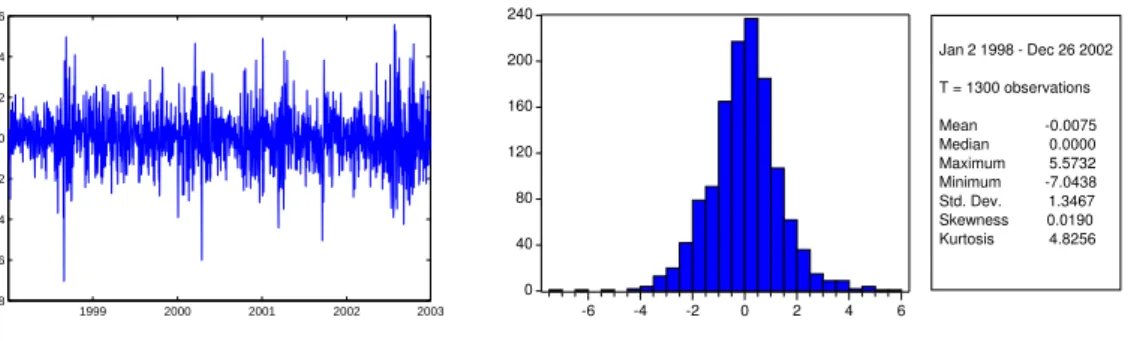
2003 2002 2001 2000 1999 −8 −6 −4 −2 0 2 4 6 0 40 80 120 160 200 240 -6 -4 -2 0 2 4 6 Jan 2 1998 - Dec 26 2002 T = 1300 observations Mean -0.0075 Median 0.0000 Maximum 5.5732 Minimum -7.0438 Std. Dev. 1.3467 Skewness 0.0190 Kurtosis 4.8256
Figure 1: S&P 500 log-returns (100×change of log-index): daily observations from1998−2002.
with ht the conditional variance ofyt given the information set It−1 ={yt−1, yt−2, yt−3, . . .}.
In addition, 0 < λ < 1, and σ2 ≡ 1/(ρ+ (1−ρ)/λ) so that var(ε
t) = 1; h0 is treated as
a known constant. We restrict ω > 0, α ≥ 0 and β ≥ 0 to ensure positivity of ht. We
follow Aus´ın and Galeano (2007) by imposing the prior restriction 0.5< λ <1, so that it is
ensured that the state with smaller variance has larger probability than the state with larger variance. We follow Aus´ın and Galeano (2007) also in specifying flat priors for the model
parameters. Moreover, we truncateω and µsuch that these have proper (non-informative)
priors. For the parameter vector θ = (ρ, λ, µ, ω, γ, α, β) of dimension k = 7 we have a
uniform prior on [0.5,1]×[0,1]×[−1,1]×[0,1]×[−1,1]×[0,1]×[0,1] withα+β <1 which
implies covariance stationarity of ht.
The returns yt are taken from the S&P 500 index. From this index we use daily
obser-vations yt (t = 1, . . . , T) on the log return (100 times the change of the logarithm of the
closing price) from January 2 1998 to December 26 2002. We chose this pre-crisis period, since the performance of the model was better than during the recent crisis. Therefore, this period is a plausible choice for this illustrative example. Figure 1 shows the returns and their corresponding descriptive statistics. This shows clearly some stylized facts of equity returns’ distributions: non-normality (excess kurtosis) and volatility clustering.
Posterior means of the model parameters are estimated by using IS and the independence chain MH algorithm. In more detail we use three candidate distributions based on
Student-t densities: the mixture of Student-t densities resulting from the MitISEM algorithm, an
‘adaptive’ Student-t distribution and a ‘naive’ Student-t distribution. The adaptive
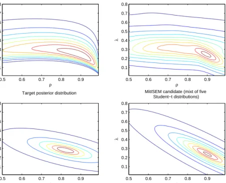
candi-date is in fact the distribution that is produced in step 1 of the MitISEM algorithm, whereas the ‘naive’ density simply uses the mode and the scale matrix estimated from the Hessian. The top left panel of Figure 2 shows the non-elliptical shapes of the posterior density.
Contour lines are plotted for (λ, ρ), where the remaining parameters are fixed at
ρ
λ
Target posterior distribution
0.5 0.6 0.7 0.8 0.9 0.1 0.2 0.3 0.4 0.5 0.6 0.7 0.8 ρ λ
MitISEM candidate (mixt of five Student−t distributions) 0.5 0.6 0.7 0.8 0.9 0.1 0.2 0.3 0.4 0.5 0.6 0.7 0.8 ρ λ
Student−t candidate (Adapted)
0.5 0.6 0.7 0.8 0.9 0.1 0.2 0.3 0.4 0.5 0.6 0.7 0.8 ρ λ
Student−t candidate (Naive)
0.5 0.6 0.7 0.8 0.9 0.1 0.2 0.3 0.4 0.5 0.6 0.7 0.8
Figure 2: Contour plots of the Gaussian Mixture GARCH (1,1) model applied toS&P 500 data. All panels show plots of the conditional (posterior/candidate) density of(ρ, λ)given(µ, ω, α, β) equal to the posterior mean (estimated by IS). The top panels depict the conditional posterior density and the candidate density contours resulting from MitISEM. The bottom panels show contours of the ‘adaptive’ and ‘naive’ candidate densities.
case λbecomes unidentified since the model does not contain a regime with larger variance
anymore. Then 1/λ, the ratio of the large and small variance, can take a wide range of
values. The remaining panels show contours of the candidate density implied by MitISEM, the ‘adaptive’ and the ‘naive’ candidate distribution. MitISEM has produced a candidate density that covers all the relevant (non-elliptically shaped) areas of the posterior target dis-tribution, whereas the adaptive and naive candidates may ‘miss’ relevant areas, for example
around points (ρ= 0.5, λ= 0.2), (ρ= 0.9, λ= 0.5) or (ρ= 0.99, λ= 0.01).
Table 1 shows posterior means estimated by the IS and MH algorithms. For both
methods, we simulate 10000 draws. For the MH approach, we take an burn-in sample of 1000 draws. Numerical standard errors (NSE) for IS and the MH algorithm are obtained by repeating the procedure 100 times. The main result from Table 1 is that MitISEM clearly outperforms the other candidate densities, irrespective whether IS or the MH method is used, since the NSE values are (much) smaller than the corresponding values implied by the Adaptive and Naive candidate densities. Regarding IS, an additional column is included
in the table: here we combine MitISEM-based IS with the variance reduction technique of antithetic sampling, where we simulate half the number of draws from the MitISEM
candidate, and for each draw the ‘mirror image’ within the Student-t component (at the
other side of the candidate Student-t component’s mode) is added. For some parameters
this leads to an improvement of the NSE, indicating that the combination of MitISEM-based IS with well-known variance reduction techniques such as antithetic sampling may
be worthwhile. However, for ρ and λ no improvement is observed, reflecting that, roughly
stated, the other side of the Student-t component may still be in a nearby subdomain of
the whole parameter space. The latter phenomenon makes the effect of antithetic sampling much less clear than under symmetric candidate distributions. We leave the combination of MitISEM with variance reduction techniques such as antithetic sampling and control variates as a topic for further research.
We end this subsection with a remark on the computing time. Given the candidate density, the IS or MH method using the MitISEM candidate costs hardly more computing
time than under a Student-t candidate. That is, the difference in computing time between
evaluating and simulating from a mixture of Student-t and a Student-t density is small, as
compared with the computing time required for the evaluation of the target density kernel. However, the construction of the MitISEM candidate necessarily requires more computing
time than the naive and adaptive Student-t candidates, since the computations for these
Student-t candidates are merely the initial steps of the MitISEM procedure.
Here, the construction of the MitISEM candidate took less than a minute (on a common laptop processor), whereas the simulation of 10000 draws requires approximately 6 seconds. From this it is clear that the MitISEM approach is especially useful if one desires estimates with a high precision. In the next subsection we will consider the Bayesian estimation of Value at Risk, where we will take a closer look at the computing time.
Table 1: Estimated posterior means and NSE’s, obtained by using three different candidate densities for IS and the independence chain MH method. NSE values of the IS method and the MH-algorithm are obtained by repeating the procedure 100 times. Maximum Likelihood estimates are provided in the first panel of the table.
Independence chain MH estimates
MitISEM Adaptive Naive
ML est. mean NSE·100 mean NSE·100 mean NSE·100
ρ 0.92 0.81 0.20 0.82 0.97 0.82 6.21 λ 0.23 0.28 0.09 0.28 0.36 0.29 1.35 µ 0.04 0.04 0.07 0.04 0.22 0.04 0.95 ω 0.06 0.09 0.12 0.08 0.27 0.09 1.31 α 0.07 0.08 0.04 0.08 0.15 0.08 0.45 β 0.90 0.87 0.06 0.87 0.23 0.86 1.05 IS estimates
MitISEM MitISEM antithetic Adaptive Naive
mean NSE·100 mean NSE·100 mean NSE·100 mean NSE·100
ρ 0.79 0.16 0.79 0.17 0.79 0.74 0.79 3.44 λ 0.28 0.08 0.28 0.08 0.28 0.15 0.28 0.66 µ 0.04 0.04 0.04 0.02 0.04 0.09 0.04 0.37 ω 0.09 0.07 0.09 0.05 0.09 0.12 0.09 0.57 α 0.08 0.03 0.08 0.02 0.08 0.05 0.08 0.28 β 0.86 0.06 0.87 0.04 0.86 0.11 0.86 0.51
2.2
Application II: efficient Bayesian forecasting of Value at Risk
In the previous subsection we illustrated that local non-identification of model parameters can cause non-elliptical shapes of the target distribution. In this subsection we will illustrate that aiming at the optimal importance density for a particular (tail-related) quantity of interest may be another cause for non-elliptical shapes of the target distribution.
A basic Bayesian procedure to multi-step-ahead prediction of Value at Risk (VaR) is as follows. Given draws of the posterior density, obtained by for example an independence chain MH algorithm, one simulates possible future paths of the returns and takes the quan-tile of interest of the simulated future returns. We label this procedure the ‘direct approach’. Hoogerheide and Van Dijk (2010) propose an indirect way to compute the multi-step-ahead VaR. They developed the approach of Quick Evaluation of Risk using Mixture of t approxi-mations (QERMit), where first the optimal importance density, derived by Geweke (1989),
qopt(·) of future returns and model parameters is approximated by a ‘hybrid’ mixture of
Importance Sampling.
The optimal importance distribution has 50% of the future returns below the VaR and 50% above the VaR; that is, 50% of the draws should consist of high losses. Therefore the
optimal importance densityqopt(·) is typically multimodal, even if the posterior is elliptically
shaped (as is the case in the Student-t GARCH model in this subsection), since it has one
mode near the mode of the future paths’ distribution (and the posterior mode) and at least one mode in the ‘high loss region’. We refer to Hoogerheide and Van Dijk (2010) for more details.
Following Hoogerheide and Van Dijk (2010), the step-by-step procedure to estimate the
τ-step ahead 100 α% VaR by the QERMit approach is as follows 1:
(Step 1) Construct an approximation of the optimal importance density:
(Step 1a) Use the MitISEM algorithm to obtain a mixture of Student-t densities q1,M it(θ)
that approximates the posterior density.
(Step 1b) Simulate a set of draws θi (i = 1, . . . , N) from the posterior distribution using
the independence chain MH algorithm with candidate q1,M it(θ). Simulate
cor-responding future paths y∗i ≡ {yi
T+1, . . . , yTi+τ} (i = 1, . . . , N) from the model
given parameter values θi and historical values y ≡ {y
1, . . . , yT}, i.e. from the
density p(y∗|θi, y). Compute a preliminary estimate V aR[
prelim as the 100 α%
quantile of the profit/loss values P L(y∗i)(i= 1, . . . , N).
(Step 1c) Use again the MitISEM algorithm to obtain a mixture of Student-t densities
q2,M it(θ, y∗) that approximates the conditional joint density of parametersθ and
future returns y∗ given that P L(y∗)<V aR[prelim.
(Step 2) Estimate the VaR using Importance Sampling with the following mixture candidate
density forθ, y∗:
ˆ
qopt(θ, y∗) = 0.5q1,M it(θ)p(y∗|θi, y) + 0.5q2,M it(θ, y∗). (20)
The first term in the candidate (20) is caused by the fact that 50% of the draws corresponding
to the ‘whole’ distribution of (θ, y∗) can be generated more efficiently by using the density
p(y∗|θi, y) that is specified by the model and approximating merely the posterior q1,M it(θ)
1There is obviously a crucial difference between the method of Hoogerheide and Van Dijk (2010) and the method described in this paper: the mixture of Student-t densities is obtained by AdMit in Hoogerheide and Van Dijk (2010), whereas we obviously use the MitISEM algorithm
than by approximating the joint distribution of (θ, y∗)2. Further, the profit/loss function
equals simply the sum of all returns y∗i in this paper.
We apply the QERMit approach by considering the 10-day ahead 99% VaR forecast
for the S&P 500 index. For estimation we use the same pre-crisis data as in the previous
subsection. We use the GARCH model (Engle (1982), Bollerslev (1986)) with Student-t
innovations: yt = µ+ut (21) ut = εt(ρht)1/2 (22) εt = Student-t(ν) (23) ρ ≡ ν−2 ν (24) ht = α0+α1u2t−1+βht−1 (25)
with Student-t(ν) the standard Student-tdistribution withνdegrees of freedom and variance
ν−2
ν . The reasons for choosing this GARCH(1,1) model with Student-t errors are that it is a
popular model among practitioners and moreover that its posterior is elliptically shaped, so that our example illustrates that flexible candidate distributions can also be useful in cases with elliptically shaped posteriors. Non-informative priors are specified for all parameters;
a proper non-informative prior is used for ν to avoid an improper posterior density; see
Bauwens and Lubrano (1998). The factorρ ensures thathtis the conditional variance ofyt.
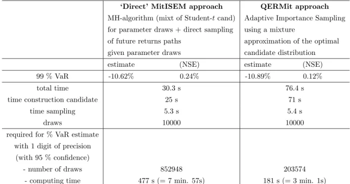
We now compare the results of the QERMit method with the ‘direct approach’ explained
at the start of this subsection. Table 2 shows simulation results. The ‘investment’ of
computing time into the construction of a candidate density for IS in case of the QERMit approach is obviously larger than for the direct approach. However, this is ‘profitable’ as the NSE of the estimated VaR – based on 10000 draws – is much smaller than the NSE of the estimator using the direct approach. As the table shows, if one wants to compute
an estimate of the VaR with a precision of 1 digit with 95% confidence, (1.96 NSE <0.05)
one needs four times more draws in the ‘direct approach’ than using the QERMit approach. This corresponds to almost eight minutes for the first approach, whereas QERMit needs only three minutes for the same precision. That is, the computational gain of QERMit
is equal to 2.64 (= 477/181). However, when one requires a higher precision this ratio
will tend to 4.11 (= 452/110), since the ‘investing time’ of constructing the candidate will
become relatively negligible. To summarize, if one needs a precise Bayesian forecast of a 2For small values of 100 (1−α)% (like the 1% or 5% percentile), the ‘whole’ distribution is close to the part of the distribution that doesnot correspond to high losses. Therefore we simulate 50% of the draws from the ‘whole’ distribution.
multi-step-ahead VaR, then the investment of computing time in an appropriate candidate
distribution – (20) with two mixtures of Student-t distributions constructed by MitISEM –
is very profitable, as also shown by Figure 3.
Table 2: Estimates of 10-day ahead 99% VaR forecast forS&P500 based on the Student-t GARCH model. Daily data are used from 1998 - 2002.
‘Direct’ MitISEM approach QERMit approach MH-algorithm (mixt of Student-tcand) Adaptive Importance Sampling for parameter draws + direct sampling using a mixture
of future returns paths approximation of the optimal
given parameter draws candidate distribution
estimate (NSE) estimate (NSE)
99 % VaR -10.62% 0.24% -10.89% 0.12%
total time 30.3 s 76.4 s
time construction candidate 25 s 71 s
time sampling 5.3 s 5.4 s
draws 10000 10000
required for % VaR estimate with 1 digit of precision
(with 95 % confidence)
- number of draws 852948 203574
- computing time 477 s (= 7 min. 57s) 181 s (= 3 min. 1s)
0 50 100 150 200 250 300 350 400 450 500 0 500 1000 1500 2000 2500 computing time (s)
precision = 1/ var(VaR est.)
Figure 3: Precision(1/var)of estimated VaR as a function of the amount of computing time for the ‘direct approach’ (green line), and the QERMit approach (steepest, red line). The horizontal blue line corresponds to a precision of 1 digit(1.96 NSE≤0.05).
2.3
Application III: accurate estimation of posterior model
prob-abilities in case of non-elliptically shaped posteriors
In this subsection we compare the posterior model probabilities of two extensions of the Gaussian Mixture GARCH (1,1) model (17)-(19), the Gaussian Mixture GJR GARCH(1,1) and the Gaussian Mixture EGARCH(1,1) model. In these models, equation (18) is replaced by the GJR specification proposed by Glosten, Jaganathan and Runkle (1993)
ht = ω+α(yt−1−µ)2+γ(yt−1 −µ)2I[yt−µ <0] +βht−1, (26) or by the EGARCH specification introduced by Nelson (1990)
log(ht) = ω+γ y√t−1−µ ht−1 +α ( |y√t−1−µ| ht−1 −E|y√t−1−µ| ht−1 ) +βlog(ht−1). (27)
Both models aim at capturing the ‘leverage-effect’, i.e. that an unexpected negative shock in the asset price boosts volatility more up than a positive shock of the same magnitude. This effect is discovered by Black (1976) and confirmed by findings of Nelson (1990) and Schwert (1990).
We have no a priori preference for one particular model, so that the posterior odds ratio is equal to the Bayes factor, the ratio of the marginal likelihoods of both models, whereas
the marginal likelihood of modelM1 is given by
p(y|M1) =
∫
p(y|θ1, M1)p(θ1|M1)dθ1 (28)
wherep(y|θ1, M1) is the likelihood of the model and p(θ1|M1) the exact prior density of the
parameters θ1 in model M1. However, since we use flat priors for the parameters of both
models, we can not directly use marginal likelihoods, due to Bartlett’s paradox (Bartlett
(1957)). In order to get reasonable model probabilities, we compute thepredictive likelihood
of both models. Eklund and Karlsson (2007) show that the sensitivity of model probabilities to the prior choice can be handled using predictive likelihoods and summarize alternative ways to specify and calculate the predictive likelihood. We compute the predictive likelihood
as follows. By splitting the datay= (y1, . . . yT) intoy∗ = (y1, . . . ym) and ˜y= (ym+1, . . . yT),
the predictive likelihood of modelM1 is given by:
p(˜y|y∗, M1) =
∫
p(˜y|θ1, y∗, M1)p(θ1|y∗, M1)dθ1, (29)
which is actually the marginal likelihood if we consider ˜y as ‘the data’ and p(θ1|y∗, M1),
the exact posterior density after observingy∗, as the prior. Using Bayes’ rule for this exact
posterior density p(θ1|y∗, M1) and substituting into (29) yields
p(˜y|y∗, M1) = ∫ p(y|θ1, M1)p(θ1|M1)dθ1 ∫ p(y∗|θ1, M1)p(θ1|, M1)dθ1 . (30)
Hence this predictive likelihood is simply the ratio of the marginal likelihood for all obser-vations over the marginal likelihood for the first part of the data.
We estimate these marginal likelihoods by IS, where we compare the performance of
the candidate density resulting from MitISEM with the ‘adaptive’ Student-t density. The
computation of apredictive likelihood may be yet another reason why one needs an
approx-imation of a non-elliptically shaped target distribution. For the posterior after observing
only the first subset of data y∗ may ‘suffer’ more from local non-identification of model
parameters than the posterior based on the whole data set y. Roughly stated, the subset
of data y∗ may not contain strong enough information to ‘keep the posterior away from
difficult areas (e.g., ridges due to local non-identification) of the parameter space.
In this application, we use again the S&P 500 data and repeat the simulation-based
computation of the predictive likelihoods, Bayes factors and model probabilities 100 times.
The first 600 observations are regarded as the ‘training sample’ y∗ = (y1, . . . ym). Table 3
shows simulation results. Two main findings arise from the table. First, the NSE values suggest that MitISEM produces far more precise estimates of predictive likelihoods and hence model probabilities. Second, an even more important result is that there is a sizeable difference between the means of the estimated predictive likelihoods from both approaches
(over the 100 repetitions). The reason is arguably that the adaptive Student-t candidate
density misses an important subdomain of the parameter space. The considerable number
of Student-t components in the mixture approximations (between 3 and 6) suggests the
presence of rather non-elliptical shapes. In future research we will investigate this difference in more detail. In any case, the example stresses that the specification of an appropriate candidate density may be relevant for estimating model probabilities, and hence for model choice or Bayesian Model Averaging.
Table 3: Model comparison between a Gaussian Mixture GJR-GARCH and a Gaussian Mixture EGARCH model. Means and corresponding NSE values are based on 100 simulation runs. Predictive likelihoods are computed by IS with adaptive Student-tand MitISEM candidate densities.
Mixt GJR-GARCH Mixt EGARCH
MitISEM results
# components Training sample 3 5
in candidate Full Sample 6 4
Predictive Likelihood
10234·mean 10236· NSE 10234·mean 10236·NSE
MitISEM 1.70 2.96 7.03 8.46
Adaptive 1.76 8.42 5.86 22.51
Bayes Factors and Model Probabilities
mean 103·NSE mean 103·NSE
Bayes Factor MitISEM 0.24 4.90
Adaptive 0.30 19.10
Model prob MitISEM 0.19 3.18
Adaptive 0.23 11.18
3
Sequential MitISEM
In this section, we propose a method for applying MitISEM in a sequential manner, so that the candidate distribution for posterior simulation is cleverly updated when new data become available. Our results show that the computational effort reduces enormously, while the quality of the approximation remains almost unchanged, as compared with an ‘ad hoc’ procedure in which the construction of the MitISEM candidate is performed ‘from scratch’ at every moment in time. In the next subsection we show how this sequential approach can be combined with a tempering approach, which facilitates the simulation from densities with multiple modes that are far apart.
The previous sections showed that, although the IS-weighted EM steps are relatively efficient, the construction of an appropriate candidate distribution may still require consid-erable computing time. After all, it requires evaluations of the target density kernel. This may seem a serious disadvantage if one requires multiple estimates over time, for example daily Bayesian forecasts. However, the idea behind the procedure in this section is that the
posterior for data y1:T+1 ={y1, . . . , yT, yT+1} is typically not so different from the posterior
for data y1:T = {y1, . . . , yT}. Therefore, one can ‘recycle’ the same candidate distribution.
At many moments, the candidate distribution can simply be reused. Further, if the can-didate distribution needs to be updated, i.e. if its quality falls below a certain level, then
we still do not require to start from scratch. It may suffice to perform an update using the
IS-weighted EM algorithm, keeping the numberH of Student-t components the same. Only
if the resulting quality is still below a desired level, then we start the MitISEM procedure, adding components until convergence has been reached.
Suppose that at time T +τ (τ = 1,2, . . .) we want to analyze the posterior based on
datay1:T+τ ={y1, . . . , yT+τ}, and that time T was the last time when we had to update the
candidate density. That is, the current candidate distribution has been estimated using the
data y1:T. Then at time T +τ we perform the following algorithm:
Algorithm 2. The Sequential MitISEM approach for obtaining a candidate density for the posterior density for data y1:T+τ:
(1) Compute C.o.V.(no update), the C.o.V. value that is based on the posterior density
kernel for datay1:T+τ and the current candidate density.
(2) Compare C.o.V.(no update) with C.o.V.(T), the C.o.V. value of the last time when
the candidate was updated. If the change is below a certain threshold (10%), stop. Otherwise go to step (3).
(3) Run the IS-weighted EM algorithm with the current mixture of H Student-t densities
as starting values. Sample from the new distribution (with the same number of
com-ponentsH) and compute IS weights and the corresponding C.o.V. value C.o.V.(only
EM update). Since the IS-weighted EM algorithm updates all mixture components, it can easily perform a useful shift of the candidate density.
(4) Judge the value of C.o.V.(only EM update). If the change of quality is below a certain
threshold (10%), stop. Otherwise go to step (5).
(5) Iterate on the number of components until the C.o.V. value has converged.
When a particular Student-t component gets a minimal weight, then the practical
rel-evance is negligible. In such a case we delete the Student-t component from the mixture.
So, the number of Student-t components is not monotonically increasing over time. In step
(2) we compare C.o.V.(no update) with C.o.V.(T) rather than the C.o.V. for the posterior
at time yT+τ−1, since in the latter case a series of small increases of the C.o.V. may
eventu-ally lead to a much worse candidate density, without the algorithm ever being ‘alarmed’ to update the candidate.
We apply the Sequential MitISEM algorithm to the Gaussian Mixture EGARCH model with the S&P 500 data. We estimate the model on the first 1300 observations and recycle the obtained candidate density by adding iteratively one observation of the forecast sample to
the existing sample. At each timet = 1301, . . . ,1350, the predictive likelihood is computed.
The training sample y∗ (for the marginal likelihood in the denominator of the predictive
likelihood) consists of 500 observations, and is remained fixed.
We compare the Sequential MitISEM approach with the ‘ad hoc MitISEM approach’,
whichs run the MitISEM algorithm from scratch at each time t = 1300, . . . ,1350. The
comparison is twofold. First we compare the computating time that is involved with both methods. Second the quality of the estimates of the predictive likelihood is compared. In order to fulfill the second comparison measure, we repeat the calculation of the predictive likelihoods 100 times and compute the NSE as the standard deviation over the repetitions. Table (4) compares both methods in computational effort and provides more details about the results of the Sequential MitISEM algorithm. During the forecast sample, the constructed candidate density is adapted only one time (step (3)). In all other cases, it was not necessary in our strategy to adapt the candidate density.
To emphasize that the number of times the candidate density is left unchanged is not a result of coincidence, we have run the Sequential MitISEM approach for a different data set and a different model. We have considered the Gaussian Mixture GJR-GARCH and Gaussian Mixture-EGARCH model, applied to daily log-returns for the SMI-index (1992-1998), data used by Aus´ın and Galeano (2007). Likewise, we iteratively add one observation
of the forecast sample to the starting sample ˜y = (y1, . . . y1000). The forecast sample is
denoted byyτ =y1001, . . . , y1858, hence 858 times the candidate density is updated, extended
or left unchanged. Table (5) shows that for both models in almost 90% of the cases the current candidate density is recycled, i.e. no adaption or extension is required.
We now turn back to the application of this section. Using the Sequential MitISEM algorithm implies a huge computational advantage, as it is more than 45 times faster than the ‘ad hoc MitISEM method’. The Sequential MitISEM algorithm is visualized in Figure
(4). The blue line representsC.o.V.(T), the Coefficient of Variation that is used in step (2)
for comparison, whereas the green line denotesC.o.V.(no update). Finally the red line gives
an impression of the quality of the ‘ad hoc MitISEM approach’: the average C.o.V. value of the ‘ad hoc MitISEM approach’ over the same period. When the dataset includes the 25th observation of the forecast sample, the new C.o.V . value is relatively too high. In this case the candidate density is updated which is shown by the upward shift of the blue line,