Big Data Flow Adjustment Using Knapsack Problem

(1)

ISSN Online: 2327-5227 ISSN Print: 2327-5219

DOI: 10.4236/jcc.2018.610003 Oct. 29, 2018 30 Journal of Computer and Communications

Big Data Flow Adjustment

Using Knapsack Problem

Eyman Yosef

1

_{, Ahmed Salama}

1

_{, M. Elsayed Wahed}

2

1_{Department of Mathematics, Faculty of Sience, Bour Said University, Bour Said, Egypt} 2_{Faculty of Computers and Informatics, Suez Canal University, Ismailia, Egypt}

Abstract

The advancements of mobile devices, public networks and the Internet of creature huge amounts of complex data, both construct & unstructured are being captured in trust to allow organizations to produce better business de-cisions as data is now pivotal for an organizations success. These enormous

amounts of data are referred to as Big Data, which enables a competitive

ad-vantage over rivals when processed and analyzed appropriately. However Big Data Analytics has a few concerns including Management of Data, Privacy & Security, getting optimal path for transport data, and Data Representation. However, the structure of network does not completely match transportation

demand, i.e., there still exist a few bottlenecks in the network. This paper

presents a new approach to get the optimal path of valuable data movement through a given network based on the knapsack problem. This paper will give value for each piece of data, it depends on the importance of this data (each piece of data defined by two arguments size and value), and the approach tries to find the optimal path from source to destination, a mathematical models are developed to adjust data flows between their shortest paths based on the 0 - 1 knapsack problem. We also take out computational experience using the commercial software Gurobi and a greedy algorithm (GA), respec-tively. The outcome indicates that the suggest models are active and worka-ble. This paper introduced two different algorithms to study the shortest path problems: the first algorithm studies the shortest path problems when sto-chastic activates and activities does not depend on weights. The second algo-rithm studies the shortest path problems depends on weights.

Keywords

0 - 1 Knapsack Problem, Big Data, Big Data Analytics, Big Dao Ta Inconsistencies

How to cite this paper: Yosef, E., Salama, A. and Wahed, M.E. (2018) Big Data Flow Ad-justment Using Knapsack Problem. Journal of Computer and Communications, 6, 30-39. https://doi.org/10.4236/jcc.2018.610003

Received: July 3, 2018 Accepted: October 26, 2018 Published: October 29, 2018

http://creativecommons.org/licenses/by/4.0/

(2)

DOI: 10.4236/jcc.2018.610003 31 Journal of Computer and Communications

1. Introduction

Big data is a big deal. We read about it and its promises of insight. But we will need a network to collect and distribute big data connected to processing loca-tions. Many big data applications require real-time communicaloca-tions. Plan for big data on your network now; don’t wait until issues arrive. Catch-up costs money and results in delayed implementations.

The only sure predictions around big data’s impact are that the network will be busier, need more capacity, and probably cost more. How much capacity will be needed is only an estimate. It could wind up being far more than estimated if the big data applications are very successful. Educated predictions on traffic may look good now, but conditions can change and render them inaccurately.

Real-time processing of big data will require real-time data delivery; data will already be old and historical. One of the advantages of big data, especially in re-gard to the Internet of Things (IoT), is its enabling of a rapid response to changing business functions and conditions such as security alerts, building au-tomation, location tracking, etc. Big data collected quickly fosters just-in-time decisions.

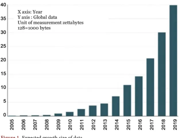
The United Nations Economic Commission for Europe predicts that data

growth will be 350% higher in 2019 than it is in 2015; Figure 1 shows the

ex-pected growth of size of data in 2019. Such volume of data means a correspond-ing 350% growth in network traffic, which may be carried over private LANs (wired and wireless) and WANs, the Internet, and cellular networks.

[image:2.595.215.529.478.719.2]

This paper proposes an applicable method to adjust the optimal path for moving big data between source and destination depending on the size and im-potence of this data, let us suppose that we have more data need to distribute through given network, according to the importance or value of each data and

(3)

total capacity of the network the approach selects the suitable amount of impor-tance data and insure that it is not exceed the total network capacity by using knapsack problem.

2. Related Work

The proposed method is concerned with specific topics of resource allocation

that have been studied in related literatures. In1996, Yu Gang [1], studied the

Max-Min Knapsack (MNK) problem as a NP-hard for an unbounded number of scenarios and pseudo polynomial solvable for a bounded number of scenarios.

The effective of lower and upper bounds were generated by surrogate relaxa-tion. The ratio of these two bounds is shown to be bounded by a constant for situations where the data range is limited to be within a fixed percentage from its mean. A branch-and-bound algorithm has been implemented to efficiently solve

the MNK problem to optimality. In 2009, Campegiani and Presti [2], suggested a

generalization model of the classical 0/1 Knapsack Problem. They developed a heuristic to obtain very near optimum solutions in a timely manner. In 2013,

Zhang et al. [3], proposed a new bio-inspired model to solve problems. The

proposed method has three main steps. First, the 0 - 1 knapsack problem is con-verted into a directed graph by the network converting algorithm. Then, for the purpose of using the amoeboid organism model, the longest path problem is transformed into the shortest path problem. Finally, the shortest path problem can be well handled by the amoeboid organism algorithm. Numerical examples are giving to illustrate the efficiency of the proposed mode. In 2015, Rooderkerk

and Heerde [4], developed a robust approach to optimize retail assortments

since retailers face the difficult task of designing a portfolio of products that balances risk and return. They proposed a novel, efficient and real-time heuristic depends on 0 - 1 Knapsack that solves the problem and offers an optimal balance. The heuristic constructs an approximation of the risk-return Efficient Frontier of assortments.

3. Knapsack Problem

3.1. The Unbounded Knapsack Problem

As a typical non-deterministic polynomial-time hard (NP-hard) problem, the unbounded knapsack problem (UKP) is defined as follows: We are given a set of

n types O=

{

o o1, , ,2 on

}

of items without quantity restriction. Items of the

same type share a common weight wiand a common value ϕi. The problem is to

choose a subset of these items aiming to maximize their overall value, while their

overall weight does not exceed a given capacity c. Without loss of generality, it

should be assumed that all values and weights are positive, all weights are

small-er than the capacity c, and the overall weight of all items exceeds c. The model of

UKP problem can be formulated as follows:

1

(4)

DOI: 10.4236/jcc.2018.610003 33 Journal of Computer and Communications 1

Constra ni

∑

in=w x ci i≤ ,

(2)

,1

i

x Z+ i n

∀ ∈ ≤ ≤

₍₃₎

where xirepresents the number of items of type oiincluded in the knapsack.

3.2. Preliminaries

In this section, the model of 0 - 1 knapsack problem and the amoeboid organism are introduced.

Mathematical model of the amoeboid organism

From the experiments on the amoeboid organism as described in [5], the

me-chanism of tube formation can be obtained: tubes thicken in a given direction when shuttle streaming of the protoplasm persists in that direction for a certain time. It implies positive feedback between flux and tube thickness, as the con-ductance of the sol is greater in a thicker channel.

According to the mechanism, two rules describing the changes in the tubular structure of the amoeboid organism are: first, open-ended tubes, which are not connected between the two food sources, are likely to disappear; second, when two or more tubes connect the same two food sources, the longer tube is likely to

disappear [6]. With these two rules, a mathematical model for maze solving

problems has been constructed.

The variable Qij is used to express the flux through tube Mij from Ni to

j

N . Assuming the flow along the tube as an approximately poiseuille flow, the

flux Qij can be expressed as [7]:

(

)

ij

ij i j

ij

D

Q p p

L

= − _{, (4)}

where pi is the pressure at the node Ni, Dij is the conductivity of the edge

ij

M .

Assume zero capacity at each node; hence by considering the conservation law

of sol the following equation can be obtained see [2]:

(

)

0, 1,2 , 1, ,

ij

Q = j≠ i= n

∑



(5)

For the source node N1 and the sink node N2 the following two equations

hold

1 0 0,

i

Q + =I

∑

(6)

2 0 0,

i

Q + =I

∑

(7)

where I0 is the flux flowing from the source node. It can be seen that I0 is a

constant value in this model.

In order to describe such an adaptation of tubular thickness we assume that

the conductivity Dij changes over time according to the flux Qij. The

follow-ing equation for the evolution of Dij can be used

(

)

d

d_tDij= f Qij −rDij

(5)

where r is a decay rate of the tube. It can be obtained that the equation implies

that the conductivity ends to vanish if there is no flux along the edge, while it is

enhanced by the flux. The f is monotonically increasing continuous function

( )

0 0

f = _.

Then the network Poisson equation for the pressure can be obtained from the

Equations (4)-(7) as follows [8]:

(

)

1 for1 for 1,2,

0 / ij i j i ij j D

p p j

L O W − =   − = + =  

∑

(9)

By setting p2=0 as a basic pressure level, all pi can be determined by

solving Equation (9) and Qij can also be obtained.

In this paper, it has been obtained that f is monotonically increasing

conti-nuous function satisfying f

( )

0 =0_{in Equation (8). Therefore,} f Q

( )

= Q _is

used in this paper. With the flux calculated, the conductivity can be derived,

where Equation (10) is used instead of Equation (8), adopting the functional

form f Q

( )

= Q _.

1

n n

ij ij n

ij D D Q D t δ + + −

= − ₍₁₀₎

3.3. Problem Description

Given an acyclic undirected network G(N,A), consisting of a set of nodes

{

1,2, ,

}

N= _ n _and_m_{undirected arcs} _{A N N}∈ × . Each arc is denoted by

or-dered pair (i, j), where i j N, ∈ _{. The weight of arc}t=

(

v vi, j

)

is denoted by a

interval data w t= = i t ti−, i+. Given two nodes vi and vt, assume P is one

path from node vi to node vt in the network G. The weight of path P is the

sum of the arcs’ weight in the path and it is stated as w(p). As a result, the

short-est path problem can be formulated as follows [9]:

( )

0 min p

( )

w p =

∑

w p

₍₁₁₎

The following equation is defined to convert

α

interval data into a crisp

number [10].

{ }

i i

(

1

)

i, 0 1

w t₌ _{= ∗ + −}

α

t−

α

_∗t+ _{≤ ≤}

α

(12)

4. A Single-Processor Machine for the 0 - 1 Knapsack

Problem in Dynamic Programming Method [11]

Dynamic Programming (DP) solves the problem by producing “ f f1, , ,2 fn”

sequentially. As mentioned in the previous section, f xi

( )

is a monotone no

lessening basic step work. “ f xi

( )

” may be exemplified as the set SPi from

claiming rows from the coordination of that phase focuses of “ f xi

( )

“.

The size of the set Si, (i.e. SPi ), is not greater than “C + 1” and rows should

be planned in growing arrangement x while f xi

( )

. The series of sets,

(6)

“Algorithm 1” to get the solution vector x see [12].

4.1 Algorithm 1- traditional 0-1 Knapsack Algorithm

Input Witem : Weight of each item ,Pitem: Profit of each item, C : Capacity

Output SP : array of subproblem to find an optimal solution, X : 0 or 1 select item or not Step 1 SPij ← {0, 0} // item : number of item , TN :total number of item Step 2 for item = 1 to TN do // Capcount: : Capacity count

For Capcount ← 0 to C do

If Witem ≤ C then // SP : subproblem

If Pitem + SPD[item -1, Capcount - Witem] > SP [item-1,Capcount] then SPD[item -1, Capcount] ← Pitem + SP[i - 1, j - Witem]

Else

SP [item , Capcount] ← SP [item -1, Capcount] // Witem > C Endif

End for // Capcount End for // item Step 3 item← TN, Capcount ← C Step 4 while item and Capcount > 0

If SP [item - 1 , Capcount] ≠ SP [item , Capcount] then item ← item-1, Capcount ← Capcount- Witem

Xtem = 1 else

item ← item-1 Xtem = 0 end if Endwhile

5. Numerical Example 1

In this section, a numerical example is used to show the efficiency of the pro-posed method.

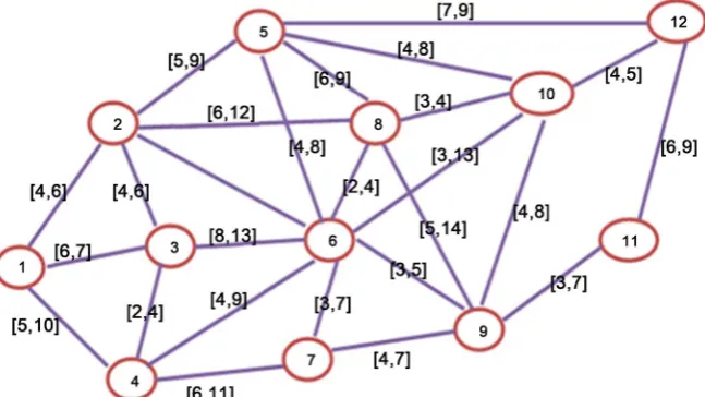
As can be seen in Figure 2, an example of shortest path problem with interval

[image:6.595.213.537.516.698.2]

arcs is shown. The shortest path from node 1 to node 12 is needed to be found,

(7)

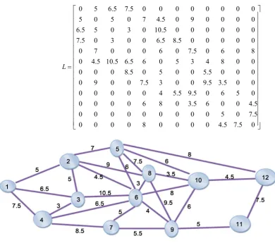
and 0≤ ≤

α

1_{, but assume that}_α_{is set 0.5,}_{Figure 3}_{can be obtained. The matrix}

corresponding to the converted graph can be obtained as follows.

From Figure 2 we can obtain this Table 1.

From Equation (12) assume all the items’ values in the initial conductivity

matrix are set α = 0.5, the shortest path from node 1 to node 12 can be found

using the amoeboid organism algorithm and the result in Table 2 obtained from

the matlab code program applied on the and Figure 3. It can be obtained that

the shortest path is (1) → (2) → (6) → (8) → (10) → (12). If α is set 1, the shortest

path in the network is (1) → (2) → (6) → (10) → (12). If α is set 0, the shortest path

in the network is 1) → (2) → (6) → (8) → (10) → (12).

It can be seen that different shortest paths are obtained when α has different

values.

6. Numerical Example 2

Consider the problem (X) with the following given data in Table 1, where n is

number of items (n = 4) and C is the total capacity (C = 5). Each item (i) has a

knapsack weight (Wi), and a knapsack profit (Pi) obtained by allocating required

[image:7.595.143.534.368.713.2]

resource to the specified item i. All Pis and Wi’s are positive integer numbers.

Table 1. The expected value to activates.

0 5 6.5 7.5 0 0 0 0 0 0 0 0

5 0 5 0 7 4.5 0 9 0 0 0 0

6.5 5 0 3 0 10.5 0 0 0 0 0 0

7.5 0 3 0 0 6.5 8.5 0 0 0 0 0

0 7 0 0 0 6 0 7.5 0 6 0 8

0 4.5 10.5 6.5 6 0 5 3 4 8 0 0

0 0 0 8.5 0 5 0 0 5.5 0 0 0

0 9 0 0 7.5 3 0 0 9.5 3.5 0 0

0 0 0 0 0 4 5.5 9.5 0 6 5 0

0 0 0 0 6 8 0 3.5 6 0 0 4.5

0 0 0 0 0 0 0 0 0 5 0 7.5

0 0 0 0 8 0 0 0 0 4.5 7.5 0

L

  

=



  

 

 _

(8)

[image:8.595.208.539.88.289.2]

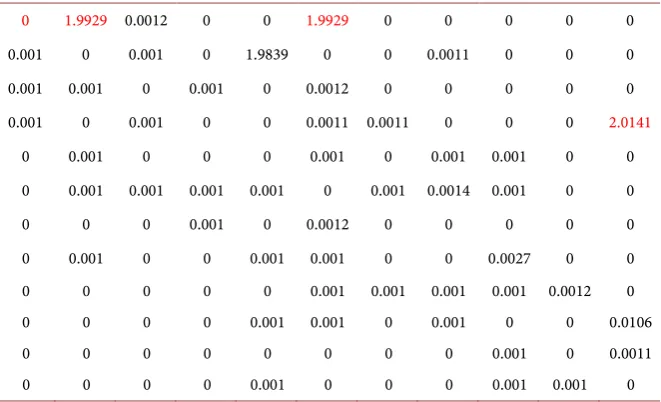
Table 2. The shortest path to network in Figure 3 (1) → (2) → (5) → (12).

0 1.9929 0.0012 0 0 1.9929 0 0 0 0 0

0.001 0 0.001 0 1.9839 0 0 0.0011 0 0 0

0.001 0.001 0 0.001 0 0.0012 0 0 0 0 0

0.001 0 0.001 0 0 0.0011 0.0011 0 0 0 2.0141

0 0.001 0 0 0 0.001 0 0.001 0.001 0 0

0 0.001 0.001 0.001 0.001 0 0.001 0.0014 0.001 0 0

0 0 0 0.001 0 0.0012 0 0 0 0 0

0 0.001 0 0 0.001 0.001 0 0 0.0027 0 0

0 0 0 0 0 0.001 0.001 0.001 0.001 0.0012 0

0 0 0 0 0.001 0.001 0 0.001 0 0 0.0106

0 0 0 0 0 0 0 0 0.001 0 0.0011

0 0 0 0 0.001 0 0 0 0.001 0.001 0

Then, the subproblem SP[TN, Capcount] in algorithm 4 will be computed to find optimal solution for the list (SP) of the n items.

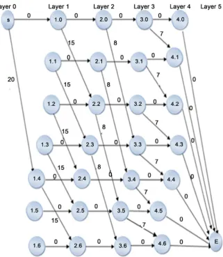
The network in the formulation has several layers of nodes: It has one layer

corresponding to each item and one layer corresponding to a source node s and

another corresponding to a sink node t. The layer corresponding to an item i has

W + 1nodes,_{i i}0 1_{, , ,}_ _iw_._Node.

The knapsack problem assuming that the knapsack has a capacity of W = 6, vj

is the value of item j, wj is the weight of item j. Figure 4 can be obtained. The

path in this graph corresponds the feasible solution of the knapsack problem.

Node S means the start node, node E means the end node. The 1st_{number in the}

residual circles means the item’s category, the 2nd_{number in these residual}

cir-cles states the capability of the knapsack that the solution has consumed. The number along the arc funds the value of the consistent item. For example the circle with rate (1, 4) in the first layer means that the item has used 4 units of the knapsack’s capacity. At the similar time, each path from node S to node E ex-plains a possible answer to the problem. For example, the path S − (1, 4) − (2, 6) − (3, 6) − (4, 6) − EE means that item 1 and item 2 are involved in the knapsack, item 3 and item 4 are omitted. It also shows that the response to the knapsack problem match the longest track in the network.

7. Conclusion

(9)

[image:9.595.217.539.70.440.2]

Figure 4. The longest path formulation of the knapsack problem with 4 items.

benchmark problems to exam the amoeboid creature algorithm. The computa-tional outcomes explain the efficiency of the presented approach. One of our outstanding studies is to solve other 0 - 1 knapsack problems under additional complex situations, such as the multi-objective shortest path problem and the knapsack problem with more criteria.

Conflicts of Interest

The authors declare no conflicts of interest regarding the publication of this pa-per.

References

[1] Gang, Y. (1996) On the Max-Min 0-1 Knapsack Problem with Robust Optimization Applications. Journal Operations Research, 44, 407-415.

https://doi.org/10.1287/opre.44.2.407

[2] Nakagaki, T., Yamada, H. and Toth, A. (2001) Path Finding by Tube Morphogene-sis in an Amoeboid Organism. Biophysical Chemistry, 92, 47-52.

(10)

DOI: 10.4236/jcc.2018.610003 39 Journal of Computer and Communications [3] Campegiani, P. and Lo Presti, F. (2009) A General Model for Virtual Machines Re-sources Allocation in Multitier Distributed Systems. ICAS ‘09. Fifth International

Conference on Autonomic and Autonomous Systems, 69, 162-167.

[4] Zhang, X., Huang, Sh., Hub, Y., Zhang, Y., Mahadevan, S. and Deng, Y. (2013) Solving 0-1 Knapsack Problems Based on Amoeboid Organism Algorithm. Applied

Mathematics and Computation, 219, 9959-9970.

https://doi.org/10.1016/j.amc.2013.04.023

[5] Robert, R.P. and Van Heerde, H.J. (2016) Robust Optimization of the 0-1 Knapsack Problem: Balancing Risk and Return in Assortment Optimization. European

Jour-nal of OperatioJour-nal Research, 250, 842-854.

https://doi.org/10.1016/j.ejor.2015.10.014

[6] Tero, A., Kobayashi, R. and Nakagaki, T. (2007) A Mathematical Model for Adap-tive Transport Network in Path Finding by True Slime Mold. Journal of Theoretical

Biology, 244, 553-564. https://doi.org/10.1016/j.jtbi.2006.07.015

[7] Ahuja, R., Magnanti, T., Orlin, J. and Weihe, K. (1995) Network Flows: Theory, Al-gorithms and Applications. ZOR - Mathematical Methods of Operations Research, 41, 252-254.

[8] Zhang, X.G., Zhang, Y.J. and Wei, D.J. (2012) Solving Shortest Path Problems with Interval Arcs Based on an Amoeboid Organism Algorithm. Journal of Information

& Computational Science, 9, 2081-2088. http://www.joics.com

[9] Zhang, G.J., Yang, H.J. and Liu, Z. (2007) Using Watering Algorithm to Find the Optimal Paths of a Maze. Computer Simulation, 24, 171-173.

[10] Nakagaki, T., Yamada, H. and Tóth, A., et al. (2000) Maze-Solving by an Amoeboid Organism. Nature, 407, 470-471. https://doi.org/10.1038/35035159

[11] Nakagaki, T., Yamada, H. and Hara, M. (2004) Smart Network Solutions in an Amoeboid Organism. Biophysical Chemistry, 107, 1-5.

https://doi.org/10.1016/S0301-4622(03)00189-3

[12] Deng, Y., Jiang, W. and Sadiq, R. (2011) Modelling Contaminant Intrusion in Wa-ter Distribution Networks: A New Similarity-Based DST Method. Expert Systems