Multiscale methods for transport phenomena

(1)

c

(2)

MULTISCALE METHODS FOR TRANSPORT PHENOMENA

BY

RAVI BHADAURIA

DISSERTATION

Submitted in partial fulfillment of the requirements

for the degree of Doctor of Philosophy in Mechanical Engineering

with a concentration in Computation Science & Engineering

in the Graduate College of the

University of Illinois at Urbana-Champaign, 2017

Urbana, Illinois

Doctoral Committee:

Professor Narayana R. Aluru, Chair and Director of Research

Professor Kenneth S. Schweizer

Professor Surya P. Vanka

(3)

Abstract

In this thesis, we discuss the development of high fidelity multiscale methods to understand fluid flow past solid interfaces. Because of the dominant surface effects at the nanoscale, the classical field based continuum models break down. Particle-based methods offer accurate insights into the flow physics but are computationally expensive. Also, the ratio of pertinent to total information (particle trajectories) from these simulations is minimal. This research entails bridging these two descriptions of the flow physics at different scales to a unified, field-based quasi-continuum framework that can provide atomic level accuracy with continuum level efficiency. First, we discuss the construction of the transport model where fluid density and transport parameters such as viscosity are assumed to be varying across the confinement. These are, in turn, incorporated using Empirical Quasicontinuum Theory (EQT) and Local Average Density Model (LADM). We elucidate the failure of the “no-slip” boundary condition at the nanoscale and its estimation using the collective diffusion coefficient from Equilibrium Molecular Dynamics (EMD) calculations. Further, we reinterpret the slip phenomenon originating from liquid-solid interfacial friction. In this context, we discuss the Generalized Langevin Equation (GLE) based single particle dynamical framework that is consistent with the EMD simulations. Our adsorption based understanding of the flow physics elucidated that the slip length does not change with the slit width. Next, the methodology of multiscale dynamical “coarse-grained” (CG) framework is further refined to incorporate multi-physics to make it viable for a variety of fluid flow situations, such as Poiseuille flow of binary mixtures and nanochannel electroosmosis. The resultant suite of multiscale models significantly reduced the computational burden from tens of thousands of hours to seconds, without trading off the accuracy of the conventional transport parameters. Finally, we demonstrate the failure of local constitutive laws in fluids when strain-rate changes appreciably compared to the fluid molecular diameter, under extreme confinement. Here, a genuinely non-local constitutive relationship between the stress and strain-rate is more appropriate, and the viscosity is interpreted as a non-local kernel instead of a material property defined pointwise. The results indicate that a non-local model performs appreciably well in capturing the strain-rate sign reversals observed from Non-Equilibrium Molecular Dynamics calculations.

(4)

(5)

Acknowledgments

I would like to thank Prof. Aluru for his countless hours of encouragement, guidance, dedication, and support during this work. Thanks to my doctoral committee members, Prof. Schweizer, Prof. Vanka, and Prof. Shukla for helpful discussions. Many thanks to National Science Foundation and Air Force Office of Scientific Research for their continued financial support during my doctoral research. I would also like to acknowledge parallel computing resources provided by the Campus Cluster and Blue Waters at the University of Illinois, and National Center for Supercomputing Applications. I am immensely thankful to all my group members for helpful discussions. In particular, I would like to mention Sikandar Mashayak, Tarun Sanghi, Kumar Kunal, Aravind Alwan, and Subhadeep De. I also acknowledge the scholars in nanofluidics community, whose literary work has helped to shape my philosophy towards this research area.

I am thankful to my friends for their time, and keeping me cheerful and motivated during my stay at Urbana-Champaign. A special thank you to Souvik Roy, Amit Desai, Sikandar Mashayak, Siddhartha Verma, Tarun Sanghi, Mohammad Heiranian, and Matthew Sylvain for the same.

I would like to thank my uncle and aunt for making me feel at home away from home. Finally, I am deeply indebted and grateful to my wife, Koyal, and my parents for their unflinching support, sacrifice, and patience.

(6)

List of Tables

2.1 LJ interaction parameters for surface and fluid atoms. C is carbon atom, C∗ is carbon atom with methane LJ energy parameter and Si is silicon atom. Fluid is LJ methane denoted by

CH4. . . 19

2.2 EQT parameters for computing density profiles.. . . 19

2.3 Parameters for exponential fithF(0)F(t)i ≈Aexp(−Bt). . . 19

3.1 Friction coefficientζ0 (kJ-ps/mol/nm2). . . 40

3.2 Slip lengths (nm) of water on different interfaces. CVG is an abbreviation for Continuum Velocity Gradient method (Eq. (1.1)), and EMD value is computed usingls=Aµ(−L/2 +δ)/ζ0 40 4.1 LJ parameters of different species used to study mixture transport. . . 60

4.2 Slip lengths (nm) of species on graphene interfaces for select methane-hydrogen mixtures. . . 60

5.1 LJ interaction parameters in MD simulations of EOF. . . 85

(9)

List of Figures

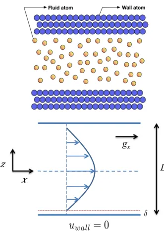
2.1 Schematic plot of the gravity driven flow considered in present work. . . 20

2.2 Density (ρ(z), top plot) and average density profiles ( ¯ρ(z), bottom plot) computed using LADM for select cases of (a) C–CH4 (8σff and 3σff), (b) C∗–CH4 (7σff and 3σff), and (c)

Si–CH4(9σffand 4σff) type systems. For density subplot, line (blue) represents EQT results,

while circles (red) represent profiles from MD simulation. . . 21

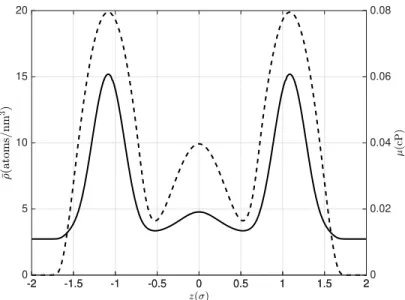
2.3 Average density (dashed, left-axis) and viscosity (bold, right-axis) for 4σffwide Si–CH4system. 22

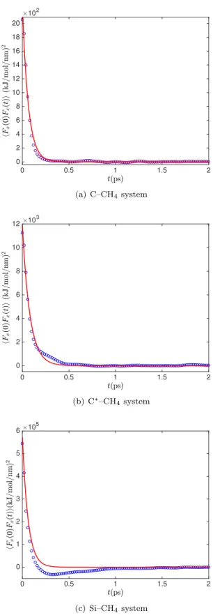
2.4 Surface-fluid total force autocorrelation from MD simulation (circles, blue) and exponential fits (bold line, red) for (a) C–CH4, (b) C∗–CH4 and (c) Si–CH4 system. . . 23

2.5 Velocity profiles for methane confined in graphene slits of size (a) 20σff, (b) 11σff, (c) 7σff and

(d) 4σff. Continuum results are in solid line (blue), while MD results are represented by error

bars (red). . . 24

2.6 Velocity profiles for methane confined in modified graphene [C∗] slits of size (a) 20σff, (b)

10σff, (c) 5σff and (d) 3σff. Continuum results are in solid line (blue), while MD results are

represented by error bars (red). . . 25

2.7 Velocity profiles for methane confined in silicon slits of size (a) 20σff, (b) 9σff, (c) 4σff and

(d) 3σff. Continuum results are in solid line (blue), while MD results are represented by error

bars (red). . . 26

2.8 Percent contribution of slip to mass flow rate (a) C–CH4 system marked with open circles

(black) and C∗–CH4 system with open squares (red) (b) Si–CH4 system with bold circles.

The lines are drawn as a guide to the data points. . . 27

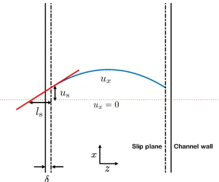
3.1 Schematic plot of the 1D transport problem illustrating slip velocityus and slip lengthls. . . 41

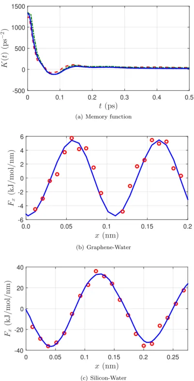
3.2 Memory function of SPC/E bulk water (blue line) at 298 K and density 33.46 molecules/nm3_.

Also plotted are memory function of water in the streaming (green dash-dot line) and confined (red dashed line) direction for 4σff wide Silicon-water system. Mean wall-fluid (solid blue line)

and total (red open circles) force in the streaming direction for (b) graphene-water, and (c) silicon-water interface. . . 42

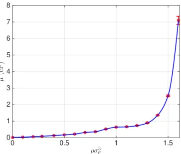
3.3 Viscosity variation of SPC/E water in centiPoise units (cP) with reduced density at 298K. Open circles (red) represent EMD data points, while solid line (blue) represents Cubic Hermite interpolation. Error bars in EMD data are of the size of the circles, except forρσff= 1.6. . . 43

3.4 Wall-fluid FACF from GLE (bold line, blue) and EMD (circles, red) for (a) graphene-water [56] and (b) silicon-water interfaces. (c) FVCCF from GLE and EMD for water with graphene and silicon interfaces.. . . 44

3.5 Velocity profiles of water in graphene slits of size (a) 20σff for gx = 1×10−4 nm/ps2, (b)

10σff for gx = 2×10−4 nm/ps 2 , (c) 7σff for gx = 5×10−4 nm/ps 2 and (d) 4σff for gx = 5×10−4 _nm/ps2

using force-field of carbon-water from Gordillo and Marti [56]. Continuum results are in solid line (blue), while MD results are represented by error bars (red). . . 45

3.6 Velocity profiles of water in silicon slits of size (a) 20σffforgx= 2×10−3nm/ps

2

, (b) 10σfffor

gx= 5×10−3nm/ps2, (c) 7σffforgx= 2×10−3nm/ps2and (d) 4σffforgx= 5×10−3nm/ps2.

(10)

3.7 Velocity profiles of water in 20σff wide (a) graphene, and (b) graphite slits using force-field

of carbon-water from Wu and Aluru [173], forgx = 10−4 nm/ps2. Continuum results are in

solid line (blue), while MD results are represented by error bars (red). . . 47

3.8 Couette flow velocity profiles of water in 20σff wide channel with uw1 = 0.1 nm/ps and

uw2 = 0.0 nm/ps. Continuum results are in solid line (blue), while MD results are represented

by error bars (red). The wall velocity is indicated by green dashed lines. . . 48

4.1 Mixture (green line, solid) and species bulk density at 1580 bar pressure and 300 K tempera-ture for different molar compositions of a methane-hydrogen mixtempera-ture. Methane is represented by blue dashed line, while hydrogen is orange dash dot line. Results are averaged over 5 NPT ensembles and errorbars are smaller than the size of the symbols. . . 61

4.2 Variation of (a) local density, (b) local average density, (c) shear viscosity, and (d) interspecies diffusion for 30–70 methane-hydrogen mixture in a 6.34 nm wide graphene slit. Mixture is represented by solid blue line, while methane is orange dash line and hydrogen is green dash dot line. The dotted red line in (d) is from bulk homogeneous EMD calculations outlined in Ref [67]. . . 62

4.3 Memory function at 300 K and 1580 bar of (a) methane in 30–70 (blue line, solid), 50–50 (red line, dash), 70–30 (green, dash-dot), and 100–0 (purple, dot), and (b) hydrogen in 70–30 (blue line, solid), 50–50 (red line, dash), 30–70 (green, dash-dot), and 0–100 (purple, dot) methane-hydrogen mixture. . . 63

4.4 Wall-fluid FACF from GLE (bold line, blue) and EMD (circles, red) for (a) methane, and (b) hydrogen in 30% methane rich mixture composition. . . 64

4.5 Methane, and (b) Hydrogen velocity profiles for 30-70 methane-hydrogen mixture. Continuum results are in solid line (blue), while MD results are represented by error bars (red). . . 65

4.6 Methane, and (b) Argon velocity profiles for 70-30 methane-argon mixture. Continuum results are in solid line (blue), while MD results are represented by error bars (red). . . 66

4.7 Methane and Hydrogen velocity profiles of 30-70 methane-hydrogen mixture with methane gravityg1= 1×10−4nm/ps2and hydrogen gravityg2= 2×10−4nm/ps2. Continuum results

are in solid line (blue), while MD results are represented by error bars (red). . . 67

4.8 Friction factor of mixture dependence on methane molar concentration in methane-hydrogen mixtures at 1580 bar and 300 K. GLE computed data points are displayed in blue open circles, while the red line is the linear least squares fit. . . 68

5.1 Density dependence of Hubbard-Onsager radius of SPC/E water at 300 K (blue circles) com-puted via EMD simulations using Eq. (5.19). Also shown (red solid line) is the 7th _order

polynomial fit to the data.. . . 86

5.2 Comparison of solvent streamwise forces for NaCl and SPC/E water system confined in silicon walls (σwall=−0.0621 C/m2). Total force (squares) contains contributions from ion-solvent,

solvent-solvent, and wall-solvent interactions. Wall-solvent (circles) include LJ and electro-static (green dashed-dot line) contributions. Also plotted is the analytical LJ force map (red solid line) computed using the method discussed in Ref. [17]. . . 86

5.3 Classical model predictions(usingµ(z) = 0.65 centiPoise) of EOF velocity profiles of NaCl-Si system for wallcharge (a)−0.0621 C/m2_{, and (b)}₋₀_._{2852 C/m}2_{. Classical results are in solid}

line (red), while MD results are represented by error bars (blue). . . 87

5.4 (a) Relative permittivity from polarization model (red line, using εr,b = 60 andµd = 4.18

Debye), and its comparison with EMD computed values (blue circles), (b) ionic conductivities, (c) ionic strength, and (d) excess viscosity for the NaCl-Si (σwall=−0.0621 C/m2) system. . 88

5.5 (a) Pure component (µP, left axis) and excess (µex, right axis) contributions to the local

vis-cosity of the solvent predicted from the model for NaCl-Si (σwall=−0.2852 C/m2). Figure (b)

shows the comparison between the model predicted (LADM + Eq. (5.8)) and EMD computed (using Stokes-Einstein relation in Eq. (5.24)) local viscosities. (c) Variation of water diffusion coefficient computed using EMD simulations. Only half-width is shown because of symmetry of profiles in thez-direction. . . 89

(11)

5.6 Wall-solvent FACF from GLE (bold line, red) and EMD (circles, blue) for (a) Na-Gr, (b) Cl-Gr, and (c) NaCl-Gr systems. . . 90

5.7 Wall-solvent (a) FACF, (b) FVCCF calculated using GLE (bold line, red) and EMD (circles, blue) for NaCl-Si (σwall = −0.0621 C/m2) system, and (c) FACF, (d) FVCCF calculated

using GLE (bold line, red) and EMD (circles, blue) for NaCl-Si (σwall=−0.2852 C/m2) system. 91

5.8 EOF velocity profiles for (a) Na-Gr, and (b) Cl-Gr systems. Continuum results are in solid line (red), while MD results are represented by error bars (blue). Insets show the viscous contributions from multiscale transport model to the EOF in more detail. . . 92

5.9 EOF velocity profiles for (a) Na-Si, and (b) Cl-Si systems. Continuum results are in solid line (red), while MD results are represented by error bars (blue).. . . 92

5.10 EOF velocity profiles for (a) NaCl-Si (σwall=−0.0621 C/m2), (b) NaCl-Gr, and (c) NaCl-Gr

using the force-field of carbon-water from Wu and Aluru [173]. Continuum results are in solid line (red), while MD results are represented by error bars (blue). Inset in (b) shows the viscous contributions from multiscale transport model to the EOF in more detail. . . 93

5.11 (top) Water (right axis) and ion (left axis) concentration profiles, and (bottom) electrical driving force across the confinement. Only half-width is shown because of symmetry of profiles in thez-direction.. . . 94

5.12 (a) Comparison of multiscale transport model EOF velocity (solid red line) with the NEMD simulations (blue circles) for NaCl-Si (σwall=−0.2852 C/m2) withExext= +0.55 V/nm. Also

plotted is the result of the transport model using EMD computed viscosity (green dash-dot line) using the Stokes-Einstein method from Eq. (5.24). Inset enhances the interfacial region. (b) Same as (a), but for KCl solution withEext

x = +0.25 V/nm.. . . 94

6.1 Shear rate dependence ofk-space viscosity for first eight modes n= 1 ton= 8. . . 106

6.2 Variation of zero shear rate k-space viscosity. STF computed data is represented by blue circles, while the red line shows a Gaussian fit. . . 106

6.3 Real space viscous kernel plotted using a Gaussian function. The red vertical lines are spaced at one molecular diameter apart to interpret the support of the kernel. . . 107

6.4 Comparison of shear stress in bulk using the local (red dashed line) and non-local (yellow solid line) model against STF-MD (blue circles) simulations for (a) fundamental mode (n= 1), and (b)n= 5. . . 107

6.5 Normalized residual vs. number of iterations for the iterative method in bulk. . . 108

6.6 Comparison of STF velocity profile predictions in bulk WCA fluid using the local (red dashed line) and non-local (yellow solid line) model against STF-MD (blue circles) simulations for (a) fundamental mode (n= 1), and (b) n= 5.. . . 108

6.7 Comparison of confined shear stress for (a) 20σff, and (b) 6σff wide slits. . . 109

6.8 Comparison of local and non-local model predicted velocity profiles against NEMD velocity profiles for (a) 20σff, and (b) 6σff wide slits. (c) compares the performance of constant vs.

(12)

Chapter 1

Introduction

1.1 Motivation

Understanding the behavior of fluids with different reagents, chemicals, and surfaces is imperative due to its role in biological and industrial processes. With the growing impetus of nanotechnology research, physics of confined fluid has generated tremendous curiosity, ranging from studying water flow in naturally occurring transmembrane protein channels like aquaporins [159,8] to artificially manufactured graphene/graphite slits and Carbon Nano Tubes (CNT) [94, 178, 93, 69, 160, 72, 81, 80, 79]. The potential applications include water purification [148, 157, 158, 79], biological flows in membranes [159, 8, 146], energy harvesting [118], and many others. These applications have instigated the need to understand the fundamental mechanism of fluid transport under confinement, both from experimental and theoretical standpoint [20].

The nature of interaction between the surface and the fluid is central to understand the flow physics [108,

31, 37], and it affects the flow in two different ways. First, competing surface and fluid interactions result in structural inhomogeneity of the fluid [137, 141, 142, 100, 98]. This structural inhomogeneity leads to spatially inhomogeneous viscosity [162, 163, 166, 27, 28]. Viscous contribution is dominant for flows in naturally occurring hydrophilic channels such as silicates [23, 52]. Second, the lattice structure and the chemical properties of the surface could result in the motion of the fluid molecules relative to the surface, a phenomenon more commonly known as slip [174, 97,168, 25]. Several experimental [94,93, 178,69] and Molecular Dynamics (MD) [72,160,79,81] studies have reported high enhancement, slip dominant flow in engineered hydrophobic surfaces. Therefore, an accurate account of both of these phenomena is critical for the development of a transport model for confined fluids.

1.2 Particle and hybrid particle-continuum based methods

Molecular dynamics (MD) simulations can provide detailed fundamental insights into the flow physics at the nanoscale. Since the pioneering work of Rahman to study liquid Argon [138], they have evolved tremendously

(13)

over the past five decades in terms of their performance, partly due to advances in computing power. In these simulations, fluid (and solids alike) are modeled as discrete particles interacting typically via an accurate albeit approximate pairwise potential field, and their trajectories are evolved using Hamilton’s equations of motion. The interparticle potentials are representative of different interaction mechanisms such as Born repulsion, van der Waals dispersion, electrostatics, bonds etc. Combined with appropriate spatial and tem-poral sampling techniques, MD can be used to study fluid structure, dynamics, and transport. Despite its rigor and accuracy, usage of MD as a predictive tool for transport phenomena is comparatively limited due to high computational requirements (massive parallelization), resulting from high degrees of freedom (number of particles) in the system. In addition, the requirement of small time steps for integrating the equations of motion due to stiff potentials restricts one to probe hydrodynamic time scales in a reasonable computational time.

The limitations of MD in probing hydrodynamic time scales can be alleviated to some extent by using softer interparticle interactions and performing a so-called “coarse-grained” dynamical simulations such as Dissipative Particle Dynamics (DPD), first proposed by Hoogerbrugge and Koelman [70]. It is an approach similar to MD regarding preserving Galilean, translational, and rotational invariance, and is widely used to perform simulations of fluid and complex systems at the mesoscale, when hydrodynamics and thermal fluctuations play a role, along with retaining the discrete nature of the interacting particles. Despite its ad-vantages, DPD has few drawbacks. First, the softening of the pairwise interaction potential term by a linear function in typical DPD simulation leads to an unphysical equation of state [59] for liquids. Furthermore, softening of the pairwise force also leads to faster dynamics, and the challenge is to address this deficiency by introducing artificial friction between the particles using a pairwise dissipative and random forces that obey the fluctuation-dissipation relationship.

Since molecular nature manifests predominantly at the liquid-solid interface, hybrid MD-continuum meth-ods can also be utilized in context to study fluid flow problems [112,61]. In these methods, MD is used to simulate the interfacial phenomenon, while the continuum based modeling approach is undertaken at the bulk-like region. The consistency of mass and momentum exchange between the two domains is maintained by introducing a buffer region, typically of the order of one molecular diameter. The attractiveness of these methods is lost due to the added complexity by adding constraints and convergence issues.

Due to the limitations mentioned above of particle-based and particle-continuum hybrid methods, there is an imperative need to address them from a continuum standpoint. Continuum field-based methods with strong foundations from atomistic or mesoscopic dynamics offer significant advantages over MD. It provides the user flexibility over the spatial resolutions, which can significantly reduce the degrees of freedom. Also,

(14)

a plethora of numerical methods (finite element, finite difference, spectral methods, etc.) can be leveraged to provide numerical solutions. For this exercise, the classical continuum-based models should be revised by embedding the microscopic physics in two ways. First, by introducing the liquid structure by incorporating particle spatial correlations such as radial distribution function, and dynamical time correlations information to ensure that the interparticle friction manifesting in the form of transport coefficients such as viscosity, diffusion, and liquid-solid interfacial friction are accurate.

1.3 Review of Transport Models

1.3.1 Constitutive relationships and viscosity models

The formulation of accurate constitutive laws governing the relationship between the stress and strain-rate is quite involved and active area of research. The earliest and simplest framework of intermolecular collision mediated momentum exchange was provided by Chapman and Cowling [39]. It relies on the Chapman-Enskog solution to the Boltzmann equation, that can describe the kinetic theory of gases in bulk. Although the kinetic theory is extremely useful for computation of transport coefficients such as viscosity, diffusion, and thermal conductivity, its usage is rather limited to monoatomic gases at low density. This is because it neglects the ternary collisions, that become important at high density cases. Also, the calculation of temper-ature dependent collision integrals becomes difficult for complex molecules. Application of different variants of kinetic theory to compute inhomogeneous transport coefficients has met with limited success [126,127,1]. Besides the above outlined attempts based on the kinetic theory to rigorously determine the inhomo-geneous transport coefficients, heuristic models such as the Local Average Density Model (LADM) can be utilized for the same purpose [28,20]. The underlying motivation of formulating LADM originates from early efforts to construct excess free energy functionals for inhomogeneous fluids in classical Density Functional Theory (c-DFT). With a specified equation of state for homogeneous (bulk) fluid, the LADM is used to obtain transport properties corresponding to the local point of interest in the homogeneous fluid. Several models for computing local average density exist in literature, such as generalized van der Waals model, hard-rod model, Tarazona model etc. The LADM has provided reasonably satisfactory estimation of the velocity profiles of confined fluids under shear driven situations [28,125]. However, the accuracy of LADM is still debated due to the lack of an explicit comparison of the local transport property provided by the LADM with the one directly obtained from the MD simulations.

At molecular length scales, however, the notion of local transport properties may not always be an accu-rate one. Close examination of the confined fluid flow velocity profiles obtained performing gravity driven

(15)

MD simulations have confirmed the nature of non-quadratic velocity profiles near the interface [1,166,164]. Furthermore, under certain circumstances, the velocity profile showed local extrema while local shear stress being a non-zero quantity, thereby challenging the validity of pointwise stress and strain-rate relationship. The viscous momentum transfer mechanism, in strictest sense, has to be reinterpreted as non-local mecha-nism instead of a local one [47]. Further studies in this context were able to characterize the non-local kernel for homogeneous fluids [63]. However, computation of a truly non-local viscous kernel for confined fluid is still an open problem [36].

1.3.2 Interfacial slip models

A general first order slip boundary condition for hydrodynamics prevalent in the literature is given as

lsdux(z) dz _z₌_δ =us, (1.1)

where z is the direction perpendicular to the confining walls,ux is the velocity field, ls is the slip length,

dux/dz is the strain rate, us is the slip velocity, which is the velocity of the fluid layer relative to the

adjoining wall, and δ is the distance from the surface to the location where the boundary condition is applied, also known as the slip plane. Slip length is defined as the distance from the slip plane where the linearly extrapolated value of the velocity is zero. Navier [107] proposed a similar form of the aforementioned slip boundary condition where the slip length depends upon the interfacial friction coefficient ζ0 and the

fluid viscosityµ0 asls=Aµ0/ζ0, whereAis the interfacial area. This relationship stems naturally from an

interfacial force balance, where the viscous force balances the wall-fluid friction force. Although significant progress has been made to understand the interfacial friction coefficient [64,30,121], the common approach is to ignore the inhomogeneity in the density and the viscosity across the confinement. Huge variations in the velocity gradient in the interfacial region can also lead to uncertainties in the computed value of slip length [88], thereby limiting the applicability of Non-Equilibrium Molecular Dynamics (NEMD) as a reliable tool to compute slip length. An exhaustive mention of these issues is given recently by Kannam et al. [90,82], where significant differences in the reported values of slip length have been highlighted.

Bhatia et al. have performed an array of studies targeting slip in meso and nano scale pores [76,77,22,18]. They have developed an oscillator model for computing transport diffusion under special case of Maxwell’s boundary condition, which is exact for low density fluids [76]. Viscous and diffusive components of flow are superimposed over each other to obtain the effective transport flux. This approach, although promising, relies on an approximation of diffuse wall boundary condition with the pore which is not always the correct

(16)

representation of the wall. To apply their work to a defect free, rigid surfaces, Smoluchowski correction factor is introduced [4], which is a complicated function of the thermodynamic state of the fluid and wall structure, and till date, only limited studies exist for its calculation [151,155].

Bocquet and Barrat have presented a statistical mechanical based model using Green-Kubo relations for calculating slip length [30, 9]. This model computes the slip length as a ratio of a phenomenological parameter, friction factor to the shear viscosity. This model can then be used in conjunction with Navier slip boundary condition [31] to obtain the velocity profile. The friction factor is inherently related to the fluctuations of wall-fluid interaction force, which can be computed from EMD simulations. Hydrodynamic location of the wall is also computed using EMD correlations, where the Navier slip condition has been applied. However, their expression for friction factor has been a subject of debate whether it does or does not include fluid-fluid viscous effects as the expression involves cross-correlations between two solvent particles [121].

Hansen et al. [64] have sought to mitigate the aforementioned deficiencies by considering the motion of interfacial region from a collective dynamics point of view. The slip boundary condition in their work is replaced by an integral boundary condition, which represents the average velocity on a slab of finite width, unlike on the liquid-solid interfacial plane. The wall-fluid friction force, therefore, balances the viscous shear forces and the additional body force. The friction coefficient is obtained using time autocorrelation of COM force, and COM force–COM velocity cross-correlations on the slab. Their transport model, however, neglects the density and viscosity variation across the confinement, and therefore results in a channel width dependent slip length, even for planar surfaces.

Recently, Huang and Szlufarska [71] have developed a Green-Kubo like expression to obtain friction coefficient from EMD simulations. They have argued that interfacial friction is not a collective quantity, but a single-particle one. The resulting expression for the friction coefficient does not involve cross-particle time correlations. The total wall-fluid friction experienced by the fluid is assumed additive from the contributions of all the interfacial particles. This hypothesis can, in principle, allow one to use single particle dynamical framework to evolve the trajectory of a representative interfacial particle that is consistent with the EMD simulations, and indeed we have leveraged this point of view to explore dynamical coarse-grained methods like GLE to compute interfacial friction.

(17)

1.4 Thesis layout

The remainder of the thesis is organized as follows. In Chapter 2, we describe the construction of a multiscale, quasi-continuum framework to predict the velocity profile of a fully developed, confined fluid, driven by a constant gravity (or acceleration) field in the streamwise direction under isothermal conditions. Unlike the classical approach (Stokes equation) where the material properties are assumed to remain constant, we allow for a continuous variation of density and viscosity fields. In this context, we briefly discuss the EQT framework to accurately predict density profile of a confined fluid by simulating Lennard-Jones (LJ) fluids confined inside slit-like channels. The viscosity variations are incorporated using the LADM approach that takes density variation as an input. The interfacial slip is modeled using the time autocorrelation of the collective wall-fluid force acting on the center of mass of the fluid, that is calculated using EMD simulations. We demonstrate the applicability of the transport model to predict the velocity profile of LJ fluids confined in low and high interfacial friction conditions. In Chapter 3, we further improve the computational efficiency of the transport model by discussing a stochastic, non-Markovian, GLE based framework to compute interfacial friction. We demonstrate the accuracy of this approach by predicting the velocity profiles of gravity-driven flow of confined water. In Chapter 4, we extend our multiscale framework to study the gravity-driven flow of binary mixtures, where species-specific momentum equations account for the interspecies diffusive momentum transfer. In Chapter 5, we use the transport model to investigate EOF, which incorporates the solvent polarization, the reduction in interfacial mobility of ions to model the viscosity enhancement near the interface. In Chapter 6, we reinterpret the viscous momentum transfer mechanism by including non-local effects in the constitutive relationship between the stress and the strain-rate. Finally, concluding remarks of this thesis are drawn in Chapter 7.

(18)

Chapter 2

A Quasi-Continuum Hydrodynamic

Model for Slit shaped Nanochannel

Flow

In this chapter, we present a hydrodynamic model which includes both the lateral and longitudinal surface effects. Spatially varying shear viscosity in the confining direction is determined using the existing correla-tions for viscosity. Slip effects are modeled using a static Langevin equation describing the center of mass (COM) motion of fluid particles [152, 153], with its stochastic force being the total wall-fluid interaction force in the streamwise direction computed from an EMD simulation. We observe that, under the same ther-modynamic state, only one EMD simulation is required to obtain parameters of Langevin model for different channel widths. The model is used to study hydrodynamics for three systems, with differing surface-fluid friction due to relative motion between surface and fluid for slit shaped nanochannels.

The rest of the chapter is organized as follows: in Sec. 2.1 we present the hydrodynamic transport model. We briefly discuss the EQT method used to calculate density profiles of fluid under confinement in slit channels. Local average density method (LADM) proposed by Bitsanis et al. [27, 28] is used with viscosity correlations presented by Woodcock [170] to obtain spatial variations of fluid viscosity as a func-tional of density. We also present the development of a generic boundary condition using Langevin type model. In Sec.2.2, necessary details of MD simulations are provided. In Sec.2.3results obtained from the hydrodynamic model are discussed and compared with NEMD simulations.

2.1 Transport model

The starting point of the transport model is the Cauchy momentum equation, which relates inertial flux to the diffusive flux and is given by

Dρmu

Dt =−∇P+∇ ·τ+f (2.1)

where D/Dt=∂/∂t+u· ∇is the material derivative,uis the velocity field, ρm is the mass density of the

fluid, P is the hydrostatic pressure, f is the body force per unit volume. τ is the deviatoric stress tensor, which relates to strain rate constitutive relation to obtain the Navier–Stokes equation for incompressible

(19)

fluids

Dρmu

Dt =−∇P+∇ ·(µ∇u) +f (2.2)

whereµis the dynamic viscosity. This can be further approximated for one-dimensional gravity driven low Reynolds number flow (see Fig.2.1) as

d dz µ(z)dux(z) dz +mρ(z)gx= 0 (2.3)

with boundary conditions

ux −L 2 +δ =ux +L 2 −δ =us (2.4)

whereux(z) is the unknown streaming direction velocity,zis the direction of confinement,xis the streaming

direction, m is the molecular mass of the fluid, ρ(z) is the number density (which relates to mass density

ρm(z) =mρ(z), and is referred as density from now on), Lis the channel width andgx is the gravity field

applied in the streaming direction. Continuity equation is already satisfied under the assumption thatuz

is identically zero. Closure to the governing equations is provided by Dirichlet boundary condition at a fixed distance δ from the surface. Inputs required for this framework are density, viscosity, magnitude of slip velocityusand the distanceδfrom the actual position of the wall, where slip condition is applied. The methods to obtain these inputs are discussed below.

2.1.1 Density profiles

We first calculate density variations along the confinement to facilitate computation of viscosity profile in the slit. Here, we use Empirical-potential based Quasicontinuum Theory (EQT) to compute the density profiles [137, 141, 142, 100,99]. EQT is a multiscale framework for fast and accurate prediction of density profile of confined fluid. It uses a continuum formulation to model the wall-fluid and fluid-fluid interaction between the atoms, and solves for the density and total potential of mean force (PMF) inside a channel in a self-consistent manner. The inputs to the EQT framework are wall-fluid, and fluid-fluid interaction parameters, average density of fluid in the slit, and channel wall density. In EQT, for a slit like channel, as shown in Fig. 2.1, density variation in the channel is modeled as a one-dimensional continuum variable expressed by 1D steady-state Nernst–Planck equation,

d dz _d_ρ₍_z₎ dz + ρ(z) kBT dU(z) dz = 0, (2.5)

(20)

with boundary conditions and integral constraint on average channel density as ρ −L 2 =ρ +L 2 = 0, (2.6a) 1 L +L/2 Z −L/2 ρ(z)dz=ρavg, (2.6b)

where U(z) is the total PMF, T is the fluid temperature, kB is the Boltzmann constant, and ρavg is the average number density of the fluid in the slit, which depends upon the thermodynamic state of the fluid, i.e., operating temperature and pressure.

The total PMF has two components, namely wall-fluid (Uwf) and fluid-fluid (Uff) PMF, resulting from interactions of wall-fluid and fluid-fluid particles, respectively, and is given by U =Uwf₊_Uff_{. Wall-fluid}

PMF is computed from the continuum approximation of the wall, obtained by suitable integration taking into account the wall structure and density (ρwall), and wall-fluid interaction parameters [156], as shown in

Eq. (2.7a). Similarly, fluid-fluid PMF in EQT can be computed by integrating the potential between the fluid particles, weighted by the fluid density, as in Eq. (2.7b),

Uwf(z) = Z V uwf(|z−r|)ρwall(r)dV, (2.7a) Uff(z) = Z V uff(|z−r|)ρ(r)dV, (2.7b)

whereuwfanduffare wall-fluid and fluid-fluid pair potentials, dV is the infinitesimal volume element centered atr, and ρ(r) is the fluid number density in the volume V, outside of which, interactions between particles is neglected. A Lennard–Jones (LJ) pair potential that describes interaction between two particles,iandj

of same or different species (wall and fluid), separated at distanceris written as

uij_LJ(r) =C ij 12 r12 − C₆ij r6 , (2.8)

where C12= 4ijσ12ij andC6 = 4ijσ6ij are LJ potential parameters. Since LJ potential is highly repulsive

at small distances, computation of fluid–fluid potential may suffer from numerical singularities, leading to spurious results, or may be rendering a very stiff, and in many cases unsolvable system of equations. To avoid this, the repulsive core is “softened” by the introduction of structurally consistent smooth potential functions and bridging them with the usual 12–6 form of the LJ potential. The fluid–fluid interactions used

(21)

in this work can be summarized as [141] uff(r) =                    0 r < Rcrit 2 P n=0 anrn Rcrit≤r < Rmin uff LJ(r) Rmin≤r < Rcut 0 r≥Rcut (2.9)

Rcrit and Rmin are parameters that define the softer repulsion and truncated core and can be obtained using an optimization algorithm. C2_{type continuity, which implies the two bridge potentials, and their first}

and second derivatives have the same value at Rmin is ensured to uniquely identify the parametersan, as

discussed in Ref. [141]. Further discussion on these parameters and their values are provided in the results section.

2.1.2 Viscosity profiles

In this section, we discuss the incorporation of viscosity variation into the hydrodynamic model. Since density in the slit channel varies with position, we capture the viscosity as a density dependent property. Density variations are used to estimate the local thermodynamic state of the fluid in confinement, and correlations for shear viscosity for bulk fluid are mapped to obtain the local viscosity. Bitsaniset al.were among the first to investigate from MD simulations the effect of density variation in velocity profiles obtained from Couette flow [27]. Few salient features of their work are

1. Viscosity must be a local function of position in the confining direction to account for the observed non-linearity in velocity profiles.

2. Density variation along the confining direction is correlated to the observed velocity profile.

3. Density profiles do not change significantly for a transport (NEMD) simulation as compared to an equilibrium (EMD) simulation for the amount of shear rates of practical interest.

Based on the above observations, the authors proposed LADM which states that the local shear viscosity, instead of being a direct function of density ρ(z), is a function of the local average number density ¯ρ(z), which is defined as ¯ ρ(r) = 6 πσ3 ff Z |r−r0_|_<σ ff/2 ρ(r0)d3r0. (2.10)

(22)

inho-density involves averaging inho-density profile at each point with appropriate weight functions [68], where the definition of local average density becomes

¯ ρ(r) = Z |r−r0_|_<σ ff/2 ω(|r−r0|)ρ(r0)d3r0, (2.11)

where the weight function ω can take various forms to deal with different thermodynamic properties of interest [44,62], and satisfies the normalization condition

Z

|r−r0_|_<σ

ff/2

ω(|r−r0|)d3r0= 1. (2.12)

In this work, we choose hard-rod model using which the local average density equation is written in one dimensional form as [167] ¯ ρ(z) = 6 σ3 ff Z |z−z0_|_<σ ff/2 _σff 2 2 −(z−z0)2 ρ(z0)dz0, (2.13)

which can then be used to obtain viscosity using suitable models for equation of state of shear viscosity. En-skog has provided a closed form expression for viscosity of fluids interacting with a hard sphere potential.[39] Similarly for LJ fluids, once an effective hard sphere diameter is calculated [60], Enskog theory can be used to predict shear viscosity. While suitable correlations such as those given in Ref. [41] exist, there are limitations on their applicability to different thermodynamic states. Corrections based on an accurate equation of state for LJ fluid have been proposed in Ref. [103], but they require empirical constants, which are different for different fluids [75].

In this work, we adopt the method proposed by Woodcock to calculate viscosity from local average den-sity [170]. A one parameter model which is valid for nearly all equilibrium states of liquid and gaseous phase for LJ fluid is used. The correlation calculates viscosity as

µ( ¯ρ∗, T∗) =µ0(T)h1 +B_µ∗ρ¯∗+CAH(1/T∗)1/3( ¯ρ∗)4i, (2.14)

where ¯ρ∗ = ¯ρσ3_ff andT∗ =kBT /ff are reduced local average density and temperature respectively, and kB

is the Boltzmann constant. µ0 is the zero density limit viscosity and is computed as

µ0= 5 16σ2 ff r mkBT π fµ Ω∗(2,2), (2.15)

(23)

where Ω∗(2,2)is collision integral, andfµis dependent upon collision integrals, which follow recursion relation

as discussed in Ref. [117]. For finite densities, additional corrections for first order dependence of viscosity on density overµ0 is done through the addition of Rainwater-Friend coefficient [50] (Bµ∗) as

B_µ∗=√2(1−(T∗)−4−T∗/8). (2.16)

CAHis the Ashurst-Hoover coefficient [6] and its value is taken as 3.025. For further details on the correlation, readers are referred to the original text in Refs. [170,117].

2.1.3 Boundary condition: Langevin model

To close the model, boundary conditions are needed. In macro-scale hydrodynamics, the use of “no-slip” condition is widely accepted, in which the relative motion between the surface and the fluid is not assumed. But at smaller scales, this phenomenological relation fails to hold. Fluid flow past a surface can exhibit relative motion between the surface and the fluid, a phenomenon known as slip [179, 161]. The degree of slippage depends on the nature of physical interaction between the surface and the fluid molecules. When fluid particles try to move past a surface, a friction force tries to retard their relative motion due to the trapping and hopping mechanism in surface-fluid potential energy map [174, 97, 168], such that the shear stress in the fluid is balanced at the interface. Topology of the surface and strength of the surface-fluid interaction relative to the applied shear gradient (Couette flow) or driving force (Poiseuille flow) dictates the slip velocity [5, 31,130,109,131]. We propose a model for computation of slip velocity for isothermal gravity driven flow using Langevin dynamics [180, 152, 153], which incorporates these effects into a time autocorrelation function of surface-fluid force in the streaming direction. We assume that the fluid slip is a collective motion of particles, which can be modeled as a lumped Brownian particle in the dissipative force field of the surface. This can be written in the form of Langevin equation [152,153] as

Mduc

dt =−ηu+F(t), (2.17)

whereM =N mis the mass of the lumped Brownian particle,N is the number of particles in the simulation box, uc is the collective velocity and F(t) is the random force acting on the particle due to the surface in

the absence of any non-equilibrium force and relates to the dissipative coefficient η from the fluctuation-dissipation theorem as η= 1 kBT ∞ Z hF(0)F(t)idt. (2.18)

(24)

Using Einstein relation [89], collective diffusion coefficientDc of the Brownian particle can be written as

Dc= kBT

η , (2.19)

which can be related to slip velocity,us, in NEMD via mobility, µmob and diffusion relationship

µmob= us

M gx

= Dc

kBT

, (2.20)

wheregx is the applied gravity. The final expression for slip velocity can be written as

us= DcM gx kBT =kBT N mgx   ∞ Z 0 hF(0)F(t)idt   −1 . (2.21)

Time autocorrelation of the total surface-fluid interaction force in the streaming direction can be computed using an equilibrium MD simulation, which is computationally less expensive to perform as compared to non-equilibrium MD simulation [30,9]. Computation of force autocorrelation is independent of width of the nanochannel, provided they are at the same thermodynamic state. This model serves as a fast and accurate tool for calculation of the slip velocity. Slip boundary condition is applied at the location of first density peak, which is the location of PMF minimum [22].

2.2 MD Simulation

We consider three types of systems to represent differing levels of friction between the surface and the fluid. The working fluid in all cases is single site methane, represented as a LJ particle. For the first (low friction) system, methane confined between rigid graphene sheets is considered. For the second system, we consider rigid graphene like structure, with the wall interaction parameter changed to that of methane (ww/kB = 148.1 K). This case is similar to the one presented by Sokhan et al. [155], and results in a

moderate friction type of a flow situation. For the third system, four layers of a rigid silicon wall oriented in [111] direction as presented in Ref. [132] is considered with ww/kB = 294.93 K, and is representative of high friction (no-slip) type boundary. All MD simulations considered here are performed at constant temperature of 300 K with a timestep of 1 fs. Lorentz-Berthelot combination rule is used to calculate the interaction parameters of surface and fluid. The number of particles in a channel is estimated using the linear superposition approximation [150,43], which provides a simpler way of computing the average density in a nanochannel. Center to center distance between the first layer of wall atoms, closest to the fluid atoms

(25)

from top and bottom walls, is defined as the channel width, and this definition is used for computing the average density in the nanochannel. Simulations are performed for channel widths 20σff to 3σff, for all the

systems studied here.

MD simulations are performed with LAMMPS [123], with working fluid as single site methane molecule. Both wall–fluid and fluid–fluid interactions are modeled with 12–6 LJ potential (see Eq. (2.8)), with param-eters reported in Table2.1. For EMD simulations, systems are equilibrated for 5 ns by simulating an NVT ensemble with Nos´e–Hoover thermostat [110] with time constant of 0.4 ps. After that, production run for 10 ns is performed, with data collected every 0.02 ps for calculating force autocorrelation. This data is divided into 1000 similar samples of 10 ps each, and the resultant force autocorrelation is averaged by the number of samples.

NEMD simulations are performed with the same force field parameters as for EMD simulations. In addition, a uniform gravity field is applied in the x-direction, with their magnitude 4×10−4 _nm/ps2 _(for

graphene wall), 2×10−3_nm/ps2_{(for modified graphene wall), and 2}_×₁₀−3_nm/ps2_{(for silicon wall, except}

for 3σff channel in this case, where 5×10−3 nm/ps2 is used for better signal to noise ratio). To control

the temperature, we again make use of the NVT ensemble with Nos´e–Hoover thermostat, only this time the thermostat is coupled to y and z directions, so that it does not interfere with the flow dynamics. We also checked that the thermostat follows the equipartition theorem, by comparing the thermal kinetic energy (computed using peculiar velocity) per particle in each direction to be equal tokBT /2. This ensures that the thermostat effect is observed in each direction due to inter-particle interactions, despite not explicitly coupling it withx-direction. Simulations are performed for 20 ns, the first 10 ns data is discarded to allow for a fully developed flow profile, and the next 10 ns data is collected at every 0.2 ps. Ten identical simulations are performed with initial velocities of particles drawn from a Maxwell distribution with different seeds, to get an error estimate on the mean velocity profile. Bins of width 0.1σff are used to compute the density

and 0.2σffare used to sample velocity profiles. For reliable statistics, a minimum of 500 fluid particles were simulated in MD system, with box lengths suitably adjusted to account for the correct average density in the channel.

2.3 Results

To test the proposed hydrodynamic model, we present here the results for three different types of systems with differing surface–fluid interaction and corrugation. We calculate the density profiles from EQT, which are used in calculating viscous component of the flow. Slip component of the flow is incorporated using

(26)

Eq. (2.21). For the low friction system (C–CH4), fluid inside the slit is in equilibrium with a bath of bulk

density (ρb) 2.138 atoms/nm3, whereas moderate friction system (C∗– CH4) is in equilibrium with bulk

fluid with densityρb= 2.936 atoms/nm3. Lastly, the high friction case (Si–CH4) is at thermodynamic state

corresponding to a bulk densityρb= 2.97 atoms/nm3. To obtain the values of parameters Rmin and Rcrit

in Eq. (2.9), we adopt the linear scaling relations proposed in Ref. [141] as a first approximation. These parameters are then fine tuned to obtain the present results. EQT parameters are reported in Table 2.2. Comparison of the density profiles in Fig.2.2between EQT and MD shows that there is a very good quan-titative match between the two methods.

Variation of the local average density ( ¯ρ) computed from EQT profile using Eq. (2.13) is also plotted in Fig.2.2. We see that the average density is weighted average form of the density, and hence shows less un-dulations in its profile. There is not much shift in the peak position between the average density and density peaks because of the nature of the chosen weight function, which provides a higher bias for |z−z0_{| →}_{0 as}

evident from Eq. (2.13). A representative plot of viscosity profile is presented for Si–CH4 system in Fig.2.3.

It should be noted that viscosity in the limit of zero average density ( ¯ρ→0) isµ→µ0, which is the dilute

gas viscosity.

The autocorrelation integral

∞ R 0

hF(0)F(t)idt is computed from the autocorrelation datahF(0)F(t)i ob-tained from EMD simulation. We assume that the autocorrelation follows exponential relaxation. A two parameter exponential function is fitted to MD autocorrelation data, and further calculations for computing the integral is done on the fitted function. This process is needed for only one slit, since they are indepen-dent of slit size, and the results presented in Fig.2.4are for 20σff channel. As evident from the plots, the maximum value of force autocorrelation hF(0)F(0)iincreases from lowest friction (C–CH4) case to highest

friction case (Si–CH4), indicating that magnitude of slip velocity should be highest in C–CH4 system and

lowest in Si–CH4system, as understood from Eq. (2.21). The parameters for exponential fit are reported in

Table2.3.

2.3.1 Low wall-fluid friction: Methane confined between graphene surfaces

Since the surface energy parameter of graphene is very low (ww/kB = 28 K) and it possesses a hexagonal

closed pack structure of sp2_{hybridized carbon with bond length of 0.142 nm compared to its diameter of 0.34}

nm, its surface landscape is very smooth. Therefore, this weakly corrugated surface results in a high degree of specular reflections of fluid particles after interaction with the wall, leading to a very little resistance to the collective motion of fluid under gravity driven flow. This physics is well captured in the results presented in Fig.2.5for various slit sizes, which demonstrate that there is a considerable amount of slip flow, reflected

(27)

by the plug-like nature of velocity profiles. It can be deduced that the viscous effects are not so important in this type of low wall-fluid friction systems. However, the contribution of slip flow decreases with increase in the slit size, where the effect of the wall subsides in the region far away from the interface, and the viscous contribution starts to increase. Slip velocity boundary condition is applied at the first peak of the density profile, which is at a distance of 0.3619 nm from the wall.

2.3.2 Moderate wall-fluid friction: Methane confined between modified

graphene surfaces

For this system, the LJ potential energy parameterwwof the wall was set equal to that of the fluid, thereby

making the wall–fluid (slip) and fluid–fluid (viscous) effects comparable to each other. The amount of slip observed in response to applied gravity is less than that of graphene-methane system (as applied gravity value for the slip case is about one order of magnitude less than that of the other two cases), but still there is a considerable amount of slip present in the velocity profiles as shown in Fig. 2.6. This can be explained by increased corrugation of the surface potential, responsible for the degree of slippage. Enhanced value of the wall-fluid interaction energy parameter results in more friction and therefore provides more resistance to the moving fluid, as compared to the low friction case. In this case, a prominent parabolic shaped velocities superimposed on a considerable amount of slip flow for larger slit size is observed (see Fig. 2.6(a)). We again observe that the effect of slip contribution increases with decreasing slit size, similar to slip case (see Figs. 2.6(a)-2.6(d)). This is due to the wall effects becoming dominant in the smaller slit size channels, because the confining surfaces are closer. Again, slip velocity boundary condition is applied at the first peak of the density profile, which is at a distance of 0.3619 nm from the wall.

2.3.3 High wall-fluid friction: Methane confined between silicon surfaces

In this case, surface structure (FCC 111, rougher than that of graphene lattice) and wall-fluid interaction energy parameter result in increased corrugation of the potential, which is non-conducive for facilitating slip. A very little amount of slip is observed as shown in Fig.2.7. This case is representative of the viscous effects dominating over slip. The velocity profiles show a parabolic type nature in larger size slits as shown in Fig. 2.7(a), while a non-parabolic velocity profile in clearly evident in Fig.2.7(b) for a slit size of 9σff, which shows undulations near the interface. Reducing the slit size further to 4σff, where no bulk type region is observed in the density profile (see Figs.2.2(c)and2.3), shows significant deviation from parabolic profile as seen from Fig. 2.7(c) which one would obtain using a constant density and viscosity. Thus, a spatially

(28)

sizes. Again, the slip velocity boundary condition is applied at 0.3239 nm, which is the first density peak location. It is observed that the match between continuum and MD results is not so good for 3σff wide

channel. This can be attributed to assumption of exponential relaxation for autocorrelation of wall–fluid interaction force (see Fig.2.4(c)). A better approximation would capture the backscattering effects in the autocorrelation, thereby reducing the value of the integral and enhanced value of slip, which currently lacks in the present approximation.

2.3.4 Mass flow rate

To test the relative contribution of slip and viscous effects in different systems, we calculate the mass flow rate, ˙m, as ˙ m= +L/2−δ Z −L/2+δ mρ(z)ux(z)dz (2.22)

The above equation assumes unit length in y-direction. To compute the slip contribution to the mass flow rate ˙ms, the profileux(z) is replaced by a constant value ofus obtained from Eq. (2.21). The ratio ˙ms/m˙

is calculated for all systems and it is observed from Fig. 2.8, that the contribution of slip in mass flow rate is highest in narrower slits. Similar trends are also observed by Bhatiaet al.in Ref. [21], where the effect of contribution of viscous flow decreases in narrower SWNT (10,10) as compared to larger SWNT (60,60). While viscous effects are important in larger slits and slip starts to become a dominant flow mechanism in narrower slits, the contribution of viscous effects still cannot be neglected since they account for about 30 percent of flow rate in high friction system at slit size of 4σff (see Fig. 2.8(b)). A constant density and viscosity based transport model would result in a very different value of mass flow rate, therefore the importance of density and viscosity variations cannot be overlooked in these cases.

In this chapter, we have developed a quasi-continuum hydrodynamic transport model for gravity driven flow in slit shaped nanopores. We have demonstrated the importance of both viscous and slip components in the velocity profile by considering three different types of systems which elucidate competition between the two phenomenon. Density profiles are used to calculate space dependent viscosity profile, using LADM method. This variation is necessary to capture the non-parabolic nature of velocity profiles as it would have been for constant density and viscosity case. A general boundary condition which takes into account the total wall-fluid interactions modeled into the static Langevin equation describing center of mass motion of fluid inside the slit is used. It is demonstrated that this boundary condition works for a spectrum of wall-fluid interaction type, and its parameters are constant for fluids confined in slit under same thermodynamic state. Furthermore, it is revealed from the velocity profiles that the slip contribution in mass flow rate increases in

(29)

all cases when the confining length is decreased, which indicates that wall-fluid effects become more dominant compared to fluid-fluid effects for smaller slit sizes. Overall, the model results in good agreement with the velocity profiles obtained from NEMD simulations, and is valid for reasonable thermodynamic states that are studied in experiments for a variety of wall-surface interactions.

(30)

Table 2.1: LJ interaction parameters for surface and fluid atoms. C is carbon atom, C∗ is carbon atom with methane LJ energy parameter and Si is silicon atom. Fluid is LJ methane denoted by CH4.

Atoms σ(nm) (kJ/mol) CH4–CH4 0.3810 1.2314 C–C 0.3400 0.2328 C∗–C∗ 0.3400 1.2314 Si–Si 0.3385 2.4522 CH4–C 0.3605 0.5354 CH4–C∗ 0.3605 1.2314 CH4–Si 0.3597 1.7377

Table 2.2: EQT parameters for computing density profiles.

System Rcrit (nm) Rmin(nm) a0(kJ/mol) a1(kJ/mol/nm) a2 (kJ/mol/nm2₎

C–CH4 0.24 0.4125 87.1561 -417.4426 492.9563

C∗– CH4 0.19 0.4095 99.1396 -475.7608 563.9083

Si–CH4 0.19 0.4170 71.4594 -341.7384 401.6761

Table 2.3: Parameters for exponential fithF(0)F(t)i ≈Aexp(−Bt). System A(kJ/mol/nm)2 _B _(1/ps)

C–CH4 2.256×103 15.710

C∗– CH4 1.186×104 12.484

(31)

!"##$"%&' (#)*+$"%&'

!

_!

"

_!

!

_"#

$

_#

(32)

-4 -2 0 2 4 0 20 40 60 -4 -2 0 2 4 0 5 10 15 20 (a) C–CH4 system -3 -2 -1 0 1 2 3 0 50 100 150 -3 -2 -1 0 1 2 3 0 10 20 30 (b) C∗_–CH4 _system -4 -2 0 2 4 0 20 40 60 80 -4 -2 0 2 4 0 10 20 30 (c) Si–CH4 system

Figure 2.2: Density (ρ(z), top plot) and average density profiles ( ¯ρ(z), bottom plot) computed using LADM for select cases of (a) C–CH4 (8σff and 3σff), (b) C∗–CH4 (7σff and 3σff), and (c) Si–CH4 (9σff and 4σff)

type systems. For density subplot, line (blue) represents EQT results, while circles (red) represent profiles from MD simulation.

(33)

-2 -1.5 -1 -0.5 0 0.5 1 1.5 2 0 5 10 15 20 -2 -1.5 -1 -0.5 0 0.5 1 1.5 2 0 0.02 0.04 0.06 0.08

(34)

0 0.5 1 1.5 2 0 2 4 6 8 10 12 14 16 18 20 102 (a) C–CH4system 0 0.5 1 1.5 2 0 2 4 6 8 10 12 10 3 (b) C∗–CH4system 0 0.5 1 1.5 2 0 1 2 3 4 5 6 10 5 (c) Si–CH4 system

Figure 2.4: Surface-fluid total force autocorrelation from MD simulation (circles, blue) and exponential fits (bold line, red) for (a) C–CH4, (b) C∗–CH4 and (c) Si–CH4 system.

(35)

-10 -5 0 5 10 0 0.05 0.1 0.15 0.2 (a) 20σff -5 0 5 0 0.02 0.04 0.06 0.08 0.1 (b) 11σff -3 -2 -1 0 1 2 3 0 0.01 0.02 0.03 0.04 0.05 0.06 0.07 0.08 (c) 7σff -2 -1 0 1 2 0 0.01 0.02 0.03 0.04 0.05 (d) 4σff

Figure 2.5: Velocity profiles for methane confined in graphene slits of size (a) 20σff, (b) 11σff, (c) 7σff and (d) 4σff. Continuum results are in solid line (blue), while MD results are represented by error bars (red).

(36)

-10 -5 0 5 10 0 0.05 0.1 0.15 0.2 (a) 20σff -5 0 5 0 0.05 0.1 0.15 (b) 10σff -2 -1 0 1 2 0 0.02 0.04 0.06 0.08 0.1 (c) 5σff -1.5 -1 -0.5 0 0.5 1 1.5 0 0.02 0.04 0.06 0.08 0.1 (d) 3σff

Figure 2.6: Velocity profiles for methane confined in modified graphene [C∗] slits of size (a) 20σff, (b) 10σff, (c) 5σff and (d) 3σff. Continuum results are in solid line (blue), while MD results are represented by error bars (red).

(37)

-10 -5 0 5 10 0 0.02 0.04 0.06 0.08 0.1 (a) 20σff -4 -2 0 2 4 0 0.005 0.01 0.015 0.02 0.025 0.03 0.035 0.04 (b) 9σff -2 -1 0 1 2 0 0.005 0.01 0.015 (c) 4σff -1.5 -1 -0.5 0 0.5 1 1.5 0 0.005 0.01 0.015 0.02 (d) 3σff

Figure 2.7: Velocity profiles for methane confined in silicon slits of size (a) 20σff, (b) 9σff, (c) 4σff and (d) 3σff. Continuum results are in solid line (blue), while MD results are represented by error bars (red).

(38)

0 5 10 15 20 75 80 85 90 95 100 (a) C–CH4 and C∗_–CH4 0 5 10 15 20 0 20 40 60 80 100 (b) Si–CH4

Figure 2.8: Percent contribution of slip to mass flow rate (a) C–CH4system marked with open circles (black)

and C∗–CH4system with open squares (red) (b) Si–CH4system with bold circles. The lines are drawn as a

(39)

Chapter 3

Interfacial Friction based

Quasi-Continuum Hydrodynamical

Model

In this chapter, we formulate a one-dimensional isothermal hydrodynamic transport model for water, which is an extension to the previous chapter. Viscosity variations in confinement are incorporated by the local average density method. Dirichlet boundary conditions are provided in the form of slip velocity that depends upon the macroscopic interfacial friction coefficient. The value of this friction coefficient is computed using a novel generalized Langevin Equation (GLE) formulation that eliminates the use of equilibrium molecular dynamics (EMD) simulation. Gravity driven flow of SPC/E water confined between graphene and silicon slit shaped nanochannels are considered as examples for low and high friction cases. The proposed model yields good quantitative agreement with the velocity profiles obtained from non-equilibrium molecular dynamics (NEMD) simulations.

3.1 Transport model

The starting point of a one-dimensional gravity driven flow in a slit channel is the Stokes equation d dz µ(z)dux(z) dz +mρ(z)gx= 0, (3.1)

with boundary conditions

ux −L 2 +δ =ux +L 2 −δ =us, (3.2)

where (x, z) are the streaming direction (direction of the flow) and the confined direction, respectively;ux(z)

is the unknown streaming velocity, m is the molecular mass of the fluid, gx is the applied gravity in the

streaming direction,ρ(z) is the number density,µ(z) is the shear viscosity, andLis the channel width. The channel walls are located at −L/2 and +L/2. Dirichlet boundary conditions are provided at a distance δ

from the wall, where the first fluid layer starts to develop after the void region near the interface, with us

(40)

mathematically equivalent set of boundary conditions for the current problem can also be written as Aµ(z)dux(z) dz _z₌₋_L/₂₊_δ =ζ0us, (3.3a) dux(z) dz z=0 = 0, (3.3b)

whereAis the interfacial area andζ0is the macroscopic interfacial friction coefficient. Eq. (3.3a), although similar to the slip boundary condition presented in Eq. (1.1), describes the force balance at the interface. At the interface, the wall shear force is balanced by the interfacial friction force, which is proportional to the relative velocity between the wall and the fluid (slip velocity). The second condition in Eq. (3.3b) is representative of the symmetry of the velocity profile at the center point of the slit channel. Integrating the Stokes equation (Eq. (3.1)) once in the region (−L/2 +δ,0) and using Eq. (3.3b), we get

−µ(z)dux(z) dz _z₌₋_L/₂₊_δ +mgx 0 Z −L/2+δ ρ(z)dz= 0. (3.4)

Now, making use of Eq. (3.3a) and observing that ρ(−L/2,−L/2 +δ) = 0, Eq. (3.4) can be reformulated to obtain an expression for the slip velocity (us) as

us=Amgx ζ0 0 Z −L/2 ρ(z)dz. (3.5)

This value of slip velocity can be used as a Dirichlet boundary condition in Eq. (3.2). Inputs required for this framework are density, viscosity, and the interfacial friction coefficientζ0. Density can be obtained from the EQT framework discussed inchapter 2. The methods to obtain the remaining inputs are discussed below.

3.1.1 Viscosity profiles

Similar to our previous approach, we compute the shear viscosity of the confined fluid using the LADM [167]. It coarse-grains the local density over one molecular diameter size, and effectively identifies a state of homogeneous fluid ( ¯ρ, T), for each locationzin the confinement. The 1D local average density is calculated as ¯ ρ(z) = 6 σ3 ff Z |z−z0_|_<σ ff/2 σ_ff 2 2 −(z−z0)2 ρ(z0) dz0, (3.6)

(41)

where σff is the Lennard-Jones (LJ) diameter of the fluid, and for SPC/E water its value is 0.317 nm. The properties of homogeneous fluids are well understood and can easily be calculated from MD. Although equations of state for these properties exist for LJ type of fluids [41, 103,170], no comprehensive database or formulae exist for the shear viscosity of bulk water. Therefore, we performed EMD simulations for bulk water and used Green-Kubo formulation to compute the shear viscosity of SPC/E water [49]. Further com-putational details are provided in Sec.3.2.

3.1.2 Interfacial friction coefficient

To compute the interfacial friction coefficientζ0, we follow the linear response theory approach presented by

Huang and Szlufarska in Ref. [71]. We first compute the friction coefficientζ₀j of an individual fluid particle

jnear the interface. Using linear response theory in conjunction with generalized Langevin equation (GLE), the Green-Kubo relation forζ₀j can be expressed in terms of equilibrium time correlation functions as

ζ₀j = ∞ Z 0 hfx,jwf(0)fx,jwf(t)idt kBT+ ∞ Z 0 hvx,j(0)fx,jwf(t)idt , (3.7) wherefwf

x,jandvx,jare the instantaneous streaming direction wall-fluid force and velocity of the particlejnear

the solid wall. The time correlation in the numerator is the single-particle wall-fluid force autocorrelation function (FACF) and denominator contains wall-fluid force–velocity cross-correlation function (FVCCF). Then, we sum the contributions from all the interfacial fluid particles to obtain the total interfacial friction coefficientζ0 as

ζ0=X

j

ζ₀j. (3.8)

The FACF and FVCCF in Eq. (3.7) can be evaluated either from EMD simulation or any other particle sampling method that can simulate the single-particle dynamical motion of confined fluids in equilibrium. Once the friction coefficient is known, the slip velocity is computed from Eq. (3.5), thereby rendering the model closed.

In this work, we discuss a GLE based simulation approach to compute the interfacial friction coefficient. The description of a particle’s motion by a GLE provides a powerful coarse-grained multiscale approach to study its equilibrium correlation functions. GLE describes the motion of a test particle in terms of dissipative

Multiscale methods for transport phenomena