Multiple Hypothesis Testing and Multiple Outlier
Identification Methods
A Thesis Submitted to the
College of Graduate Studies and Research
in Partial Fulfillment of the Requirements
for the Degree of
Doctor of Philosophy
in the
Department of Mathematics and Statistics
University of Saskatchewan
Saskatoon, Saskatchewan
By
Yaling Yin
March 2010
c
Permission to Use
In presenting this thesis in partial fulfilment of the requirements for a Postgraduate degree from the University of Saskatchewan, I agree that the Libraries of this University may make it freely available for inspection. I further agree that permission for copying of this thesis in any manner, in whole or in part, for scholarly purposes may be granted by the professor or professors who supervised my thesis work or, in their absence, by the Head of the Department or the Dean of the College in which my thesis work was done. It is understood that any copying or publication or use of this thesis or parts thereof for financial gain shall not be allowed without my written permission. It is also understood that due recognition shall be given to me and to the University of Saskatchewan in any scholarly use which may be made of any material in my thesis.
Requests for permission to copy or to make other use of material in this thesis in whole or part should be addressed to:
Head of the Department of Mathematics and Statistics University of Saskatchewan
Saskatoon, Saskatchewan Canada
Abstract
Traditional multiple hypothesis testing procedures, such as that of Benjamini and Hochberg, fix an error rate and determine the corresponding rejection region. In 2002 Storey proposed a fixed rejection region procedure and showed numerically that it can gain more power than the fixed error rate procedure of Benjamini and Hochberg while control-ling the same false discovery rate (FDR). In this thesis it is proved that when the number of alternatives is small compared to the total number of hypotheses, Storey’s method can be less powerful than that of Benjamini and Hochberg. Moreover, the two procedures are compared by setting them to produce the same FDR. The difference in power between Storey’s procedure and that of Benjamini and Hochberg is near zero when the distance between the null and alternative distributions is large, but Benjamini and Hochberg’s pro-cedure becomes more powerful as the distance decreases. It is shown that modifying the Benjamini and Hochberg procedure to incorporate an estimate of the proportion of true null hypotheses as proposed by Black gives a procedure with superior power.
Multiple hypothesis testing can also be applied to regression diagnostics. In this thesis, a Bayesian method is proposed to test multiple hypotheses, of which theith null and alter-native hypotheses are that theith observation is not an outlier versus it is, fori= 1,· · · , m. In the proposed Bayesian model, it is assumed that outliers have a mean shift, where the proportion of outliers and the mean shift respectively follow a Beta prior distribution and a normal prior distribution. It is proved in the thesis that for the proposed model, when there exists more than one outlier, the marginal distributions of the deletion residual of the ith observation under both null and alternative hypotheses are doubly noncentral t
distributions. The “outlyingness” of theith observation is measured by the marginal pos-terior probability that the ith observation is an outlier given its deletion residual. An importance sampling method is proposed to calculate this probability. This method re-quires the computation of the density of the doubly noncentral F distribution and this
is approximated using Patnaik’s approximation. An algorithm is proposed in this thesis to examine the accuracy of Patnaik’s approximation. The comparison of this algorithm’s output with Patnaik’s approximation shows that the latter can save massive computation time without losing much accuracy.
The proposed Bayesian multiple outlier identification procedure is applied to some sim-ulated data sets. Various simulation and prior parameters are used to study the sensitivity of the posteriors to the priors. The area under the ROC curves (AUC) is calculated for each combination of parameters. A factorial design analysis on AUC is carried out by choosing various simulation and prior parameters as factors. The resulting AUC values are high for various selected parameters, indicating that the proposed method can identify the majority of outliers within tolerable errors. The results of the factorial design show that the priors do not have much effect on the marginal posterior probability as long as the sample size is not too small.
In this thesis, the proposed Bayesian procedure is also applied to a real data set ob-tained by Kanduc et al. in 2008. The proteomes of thirty viruses examined by Kanduc et al. are found to share a high number of pentapeptide overlaps to the human proteome. In a linear regression analysis of the level of viral overlaps to the human proteome and the length of viral proteome, it is reported by Kanducet al. that among the thirty viruses, hu-man T-lymphotropic virus 1, Rubella virus, and hepatitis C virus, present relatively higher levels of overlaps with the human proteome than the predicted level of overlaps. The results obtained using the proposed procedure indicate that the four viruses with extremely large sizes (Human herpesvirus 4, Human herpesvirus 6, Variola virus, and Human herpesvirus 5) are more likely to be the outliers than the three reported viruses. The results with the four extreme viruses deleted confirm the claim of Kanduc et al.
Acknowledgements
First of all, the author would like to express her sincere appreciation and gratitude to her co-supervisors, Dr. M. G. Bickis and Dr. C. E. Soteros for their invaluable guidance, patience, encouragement and support throughout the course of this research work and in the preparation of this thesis. The author has greatly benefited from Dr. M. Bickis and Dr. C. E. Soteros in-depth knowledge of statistics and programming.
The author’s thanks are extended to the advisory committee members, Dr. A. Kusalik, Dr. W. H. Laverty, Dr. J. R. Martin, and Dr. R. Srinivasan for their advice and guidance. The author would like to take this opportunity to acknowledge the constant encour-agement, patience and support from her parents, Guoqiang Yin and Anna Cheng and husband, Po Hu throughout her Ph.D. program. The author presents this thesis as a gift to them.
Financial assistances from the College of Graduate Studies and Research in the form of a Ph. D. Scholarship, from the Department of Mathematics and Statistics at the Uni-versity of Saskatchewan in the form of a Graduate Teaching Assistantship, and from her co-supervisors’ NSERC (Natural Science and Engineering Research Council of Canada) Discovery Grants in the form of a Research Assistantship are gratefully acknowledged.
Table of Contents
Permission to Use i
Abstract ii
Acknowledgements iv
Table of Contents v
List of Tables vii
List of Figures ix
List of Abbreviations xii
List of Symbols xiii
1 Introduction 1
1.1 Motivation . . . 1
1.2 Single Hypothesis Testing Problem . . . 3
1.2.1 Frequentist Hypothesis Testing . . . 4
1.2.2 Bayesian Hypothesis Testing . . . 8
1.3 Multiple Hypothesis Testing Problem . . . 10
1.3.1 Problem Statement and Definitions of Compound Error Measures . 10 1.3.2 Multiple Comparison Methods . . . 14
1.3.3 Multiple Hypothesis Testing Methods Based on Sequentialp-values . 15 1.3.4 Mixture models for multiple hypothesis testing . . . 21
1.4 Regression diagnostics . . . 26
1.4.1 Linear regression model and Least Squares . . . 26
1.4.2 Identification of one outlier . . . 29
1.4.3 Review of methods for identifying multiple outliers in regression . . 34
1.4.4 ROC curves and AUC . . . 36
1.5 Scope of the thesis . . . 36
2 A clarifying comparison of methods for controlling the false discovery rate 39 2.1 Introduction . . . 39
2.2 Concepts and Notation . . . 41
2.3 Clarification of the relationship between BH and FSL . . . 45
2.5 A fair comparison of BH andFSL . . . 62
2.6 Discussion . . . 66
3 Multiple deletion diagnostics 71 3.1 Introduction . . . 71
3.2 Distribution of the deletion residual when there is more than one outlier . . 74
3.3 A Bayesian approach for multiple deletion diagnostics . . . 79
3.3.1 Model description . . . 79
3.3.2 Posterior distributions . . . 83
3.3.3 Computational implementation . . . 85
3.4 Computing doubly noncentral F density . . . 87
3.5 Simulation study . . . 104
3.5.1 Simulation study of single datasets . . . 105
3.5.2 Simulation study of multiple datasets . . . 122
3.5.3 Study of factorial design . . . 141
3.6 Summary . . . 150
4 Amino acid sequence similarity of viral to human proteomes (An ap-plication of the Bayesian method proposed in Chapter 3) 153 4.1 Introduction . . . 153
4.2 Description of the dataset . . . 154
4.3 Analysis of the dataset . . . 159
4.3.1 Analysis of the full dataset . . . 159
4.3.2 Analysis of the reduced dataset . . . 169
4.4 Conclusion . . . 176
5 Conclusions and future work 178 5.1 Conclusions . . . 178
5.2 Future Work . . . 183
A Proof 195 B Tables 197 C Code 200 C.1 Code for Algorithm 3.3.1 . . . 200
List of Tables
1.1 All possible outcomes of m hypothesis tests. . . 11 2.1 Simulation estimates of π0 by using different estimates of λ. . . 48
2.2 Simulation estimates of FDR and power for BH, FSL and AFDR for m =
1000, µ= 2 and γ = 0.01,0.001. . . 49
2.3 Simulation estimates of FDR and power for BH, FSL and AFDR for m =
100, µ= 2 and γ = 0.01,0.001. . . 50
2.4 Simulation estimates of FDR and power for BH, FSL and AFDR for m =
1000, µ= 2 and γ = 0.0005,0.0001. . . 51
2.5 Simulation estimates of FDR and power for BH, FSL and AFDR for m =
100, µ= 2 and γ = 0.0005,0.0001. . . 52
2.6 Simulation estimates of FDR and power for BH, FSL and AFDR for m =
1000, µ= 1 and γ = 0.01,0.001. . . 53
2.7 Simulation estimates of FDR and power for BH, FSL and AFDR for m =
100, µ= 1 and γ = 0.01,0.001. . . 54
2.8 Simulation estimates of FDR and power for BH, FSL and AFDR for m =
1000, µ= 1 and γ = 0.0005,0.0001. . . 55
2.9 Simulation estimates of FDR and power for BH, FSL and AFDR for m =
100, µ= 1 and γ = 0.0005,0.0001. . . 56 3.1 True value and Patnaik’s approximation of the density of Fν′′1,ν2(ζ, η) with
x= 0.001, ν2= 97. . . 100
3.2 True value and Patnaik’s approximation of the density of Fν′′1,ν2(ζ, η) with
x= 0.01, ν2= 97. . . 100
3.3 True value and Patnaik’s approximation of the density of Fν′′1,ν2(ζ, η) with
x= 1, ν2= 97. . . 101
3.4 True value and Patnaik’s approximation of the density of Fν′′1,ν2(ζ, η) with
x= 10, ν2 = 97. . . 101
3.5 True value and Patnaik’s approximation of the density of F′′
ν1,ν2(ζ, η) with x= 0.001, ν2= 47. . . 101
3.6 True value of the density of doubly noncentral F withx= 0.01,ν2= 47 and
variousξ andη, and Difference = (Patnaik’s approximation− true value). . 102 3.7 True value and Patnaik’s approximation of the density of Fν′′1,ν2(ζ, η) with
x= 1, ν2= 47. . . 102
3.8 True value and Patnaik’s approximation of the density of Fν′′1,ν2(ζ, η) with
x= 10, ν2 = 47. . . 102
3.9 True value and Patnaik’s approximation of the density of Fν′′1,ν2(ζ, η) with
3.10 True value and Patnaik’s approximation of the density of F′′
ν1,ν2(ζ, η) with x= 0.01, ν2= 17. . . 103
3.11 True value and Patnaik’s approximation of the density of Fν′′1,ν2(ζ, η) with
x= 1, ν2= 17. . . 103
3.12 True value and Patnaik’s approximation of the density of Fν′′1,ν2(ζ, η) with
x= 10, ν2 = 17. . . 104
3.13 Comparison of Patnaik’s approximation and Algorithm 3.4.2 forV = 36. . . 113 3.14 Comparison of Patnaik’s approximation and Algorithm 3.4.2 forV = 16. . . 114 3.15 Comparison of Patnaik’s approximation and Algorithm 3.4.2 forV = 9. . . 114 3.16 Comparison of Patnaik’s approximation and Algorithm 3.4.2 forV = 4. . . 115 3.17 Factorial Design 1 on the AUC values calculated from simulated data sets. . 142 3.18 ANOVA table for Factorial Design 1. . . 144 3.19 Table of the means of main effects for Factorial Design 1. . . 145 3.20 Part I of the table of the means of two-way interactions for Factorial Design 1.145 3.21 Part II of the table of the means of two-way interactions for Factorial Design
1. . . 146 3.22 Factorial Design 2 on the AUC values calculated from simulated data sets
without m= 20. . . 146 3.23 ANOVA table for Factorial Design 2. . . 148 3.24 Table of the means of main effects for Factorial Design 2. . . 150 4.1 Description of the viral proteomes analyzed for similarity to human proteins. 155 4.2 Pentapeptide overlap between viral and human proteomes. . . 157 B.1 Comparison of Patnaik’s approximation and Algorithm 3.4.2 forV = 36. . . 197 B.2 Comparison of Patnaik’s approximation and Algorithm 3.4.2 forV = 16. . . 198 B.3 Comparison of Patnaik’s approximation and Algorithm 3.4.2 forV = 9. . . 198 B.4 Comparison of Patnaik’s approximation and Algorithm 3.4.2 forV = 4. . . 199
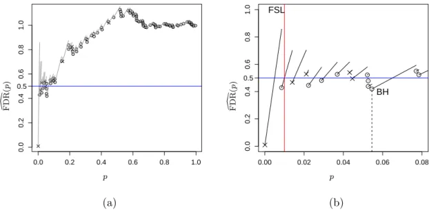
List of Figures
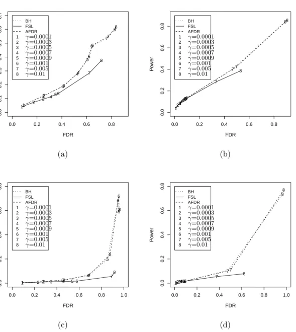
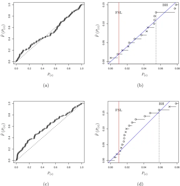
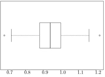
2.1 A simulated example of Storey’sFDR as a function of the significance leveld p. 44 2.2 A simulated example of Storey’sFDR as a function of the significance leveld p. 46 2.3 Relationship between power and false discovery rate for three methods. . . 58 2.4 Empirical distribution plots of p-values calculated from two datasets. . . 60 2.5 Boxplot of untruncated ˆπ0for the cases in which BH rejects more hypotheses
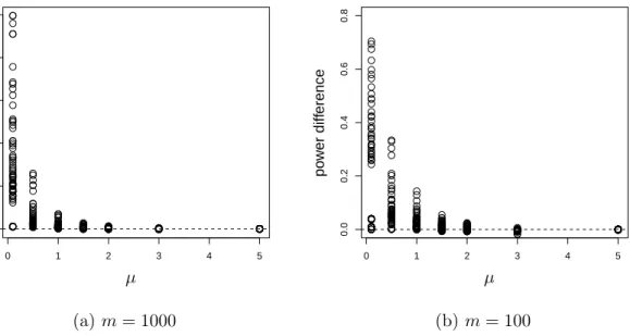
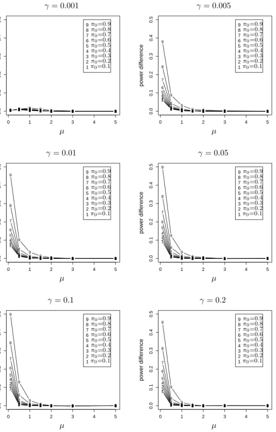
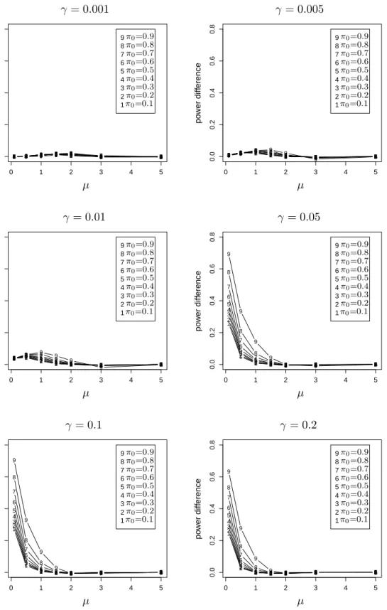
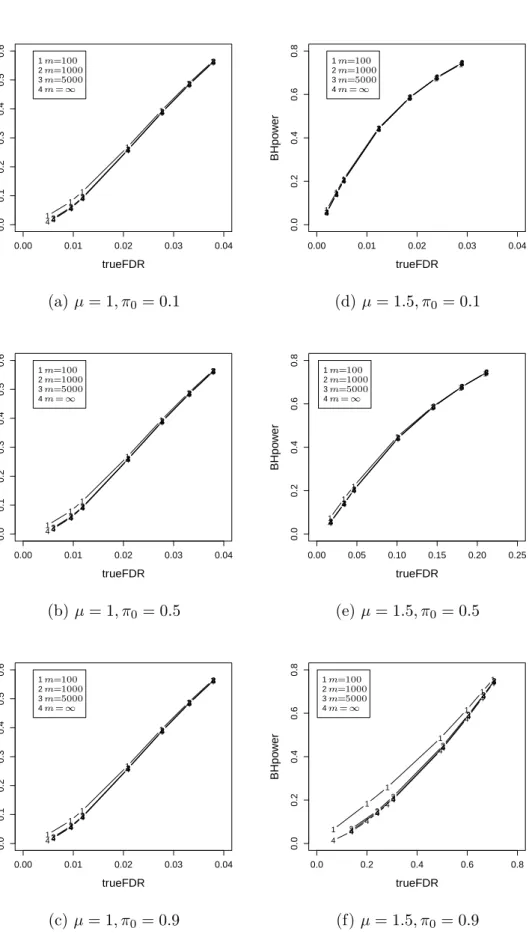
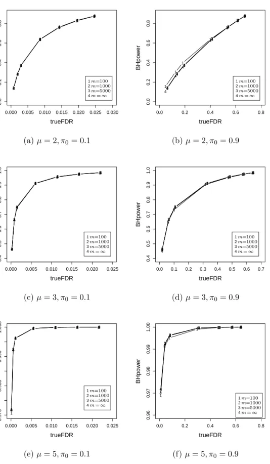
than FSL. . . 61 2.6 The power advantage of BH over FSL when the true FDR is fixed at the
same level. . . 63 2.7 The difference between the powers of the two methods versusµform= 1000. 64 2.8 The difference between the powers of the two methods versus µform= 100. 65 2.9 Relationship between power and true FDR of BH for different m. . . 67 2.10 Relationship between power and true FDR of BH for differentm. . . 68 2.11 Relationship between power and true FDR of BH for differentm. . . 69 3.1 The scatter plot and residual plot of a dataset with 100 points, of which 10
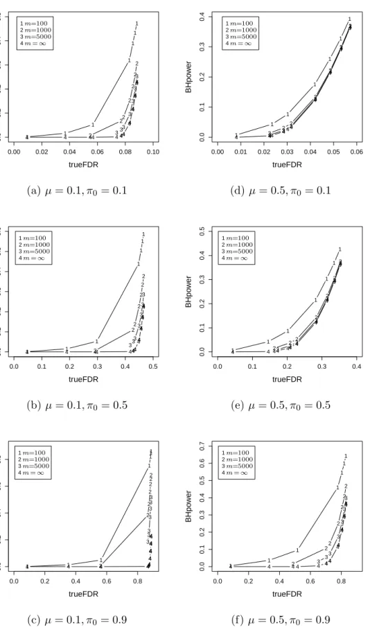
outliers have mean shifts simulated from N(0,1). . . 106 3.2 P(Hi = 1 |r∗i2) as a function ofri∗2 forV = 36 and six Beta priors onπ0. . 108
3.3 P(Hi = 1 |r∗i2) as a function ofri∗2 forV = 16 and six Beta priors onπ0. . 109
3.4 P(Hi = 1 |r∗i2) as a function ofri∗2 forV = 9 and six Beta priors onπ0. . . 110
3.5 P(Hi = 1 |r∗i2) as a function ofri∗2 forV = 4 and six Beta priors onπ0. . . 111
3.6 ROC curve for the dataset shown in Figure 3.1 with V = 36 and six Beta priors on π0. . . 117
3.7 ROC curve for the dataset shown in Figure 3.1 with V = 16 and six Beta priors on π0. . . 118
3.8 ROC curve for the dataset shown in Figure 3.1 with V = 9 and six Beta priors on π0. . . 119
3.9 ROC curve for the dataset shown in Figure 3.1 with V = 4 and six Beta priors on π0. . . 120
3.10 The scatter plot and residual plot of a dataset with 100 points, of which 10 outliers have mean shifts simulated from N(0,9). . . 121 3.11 P(Hi = 1 |r∗i2) as a function ofri∗2 forV = 36 and six Beta priors onπ0. . 123
3.12 P(Hi = 1 |r∗i2) as a function ofri∗2 forV = 16 and six Beta priors onπ0. . 124
3.13 P(Hi = 1 |r∗i2) as a function ofri∗2 forV = 9 and six Beta priors onπ0. . . 125
3.14 P(Hi = 1 |r∗i2) as a function ofri∗2 forV = 4 and six Beta priors onπ0. . . 126
3.15 ROC curve for the dataset shown in Figure 3.10 withV = 36 and six Beta priors on π0. . . 127
3.16 ROC curve for the dataset shown in Figure 3.10 withV = 16 and six Beta priors on π0. . . 128
3.17 ROC curve for the dataset shown in Figure 3.10 with V = 9 and six Beta
priors on π0. . . 129
3.18 ROC curve for the dataset shown in Figure 3.10 with V = 4 and six Beta priors on π0. . . 130
3.19 True positive rate averaged over 1000 datasets versus false positive rate averaged over 1000 datasets for V = 36 and six Beta priors onπ0. . . 132
3.20 True positive rate averaged over 1000 datasets versus false positive rate averaged over 1000 datasets for V = 16 and six Beta priors onπ0. . . 133
3.21 True positive rate averaged over 1000 datasets versus false positive rate averaged over 1000 datasets for V = 9 and six Beta priors onπ0. . . 134
3.22 True positive rate averaged over 1000 datasets versus false positive rate averaged over 1000 datasets for V = 4 and six Beta priors onπ0. . . 135
3.23 True positive rate averaged over 1000 datasets versus false positive rate averaged over 1000 datasets for V = 36 and six Beta priors onπ0. . . 137
3.24 True positive rate averaged over 1000 datasets versus false positive rate averaged over 1000 datasets for V = 16 and six Beta priors onπ0. . . 138
3.25 True positive rate averaged over 1000 datasets versus false positive rate averaged over 1000 datasets for V = 9 and six Beta priors onπ0. . . 139
3.26 True positive rate averaged over 1000 datasets versus false positive rate averaged over 1000 datasets for V = 4 and six Beta priors onπ0. . . 140
3.27 Residual vs. fitted value plots for the factorial design in Table 3.17. . . 147
3.28 Residual vs. fitted value plots and normal QQ plots of the residuals for Factorial Design 1 and Factorial Design 2. . . 149
4.1 The scatter plot of the viral pentapeptide overlap including duplicates in the human proteome versus the unique pentapeptide in the viral proteome for the full dataset. . . 158
4.2 P(Hi = 1 |r∗i2) as a function ofri∗2 forV = 36 and six Beta priors onπ0. . 160
4.3 P(Hi = 1|ri∗2) as a function ofr∗i2 forV = 16 and six different Beta priors on π0. . . 161
4.4 P(Hi = 1 |r∗i2) as a function ofri∗2 forV = 9 and six Beta priors onπ0. . . 162
4.5 P(Hi = 1 |r∗i2) as a function ofri∗2 forV = 4 and six Beta priors onπ0. . . 163
4.6 The magnified lower ends of plots (a) - (f) of Figure 4.2. . . 165
4.7 The magnified lower ends of plots (a) - (f) of Figure 4.3. . . 166
4.8 The magnified lower ends of plots (a) - (f) of Figure 4.4. . . 167
4.9 The magnified lower ends of plots (a) - (f) of Figure 4.5. . . 168
4.10 The scatter plot of the viral pentapeptide overlap including duplicates in the human proteome versus the unique pentapeptides in the viral proteome for the reduced dataset. . . 170
4.11 P(Hi = 1| ri∗2) as a function of r∗i2 forV = 36 and six Beta priors on π0 for the reduced dataset. . . 172
4.12 P(Hi = 1| ri∗2) as a function of r∗i2 forV = 16 and six Beta priors on π0 for the reduced dataset. . . 173
4.13 P(Hi = 1|r∗i2) as a function ofr∗i2 forV = 9 and six Beta priors on π0 for the reduced dataset. . . 174
4.14 P(Hi = 1|r∗i2) as a function ofr∗i2 forV = 4 and six Beta priors on π0 for the reduced dataset. . . 175
List of Abbreviations
AFDR Adaptive FDR controlling procedure
AUC Area under ROC Curve
BH Benjamini and Hochberg procedure
EL extremely large viruses
FDP False discovery proportion
FDR False discovery rate
FEL four extremely large (viruses)
FNP False non-discovery proportion
FNR False non-discovery rate
FPR False positive rate
FSL Fixed significance level procedure
FWER Family-wise error rate
k-FWER k-Family-wise error rate
KI Kanduc et al. identified (viruses)
MCMC Markov chain Monte Carlo
MMLE Marginal maximum likelihood estimate
MPT Most powerful test
MVN multivariate normal (distribution)
PCER Per comparison error rate
PFER Per family error rate
pFDR Positive false discovery rate
pFNR Positive false non-discovery rate
PFP Proportion of false discoveries (positives)
ROC Receiver operating characteristic
TPR True positive rate
List of Symbols
∼ a random variable follows a certain distribution
φ the density of the standard normal distribution
Φ the CDF of the standard normal distribution
m the total number of tests
n the number of iterations in a simulation study or the number of
random samples generated by using a Monte Carlo method
m0 the number of true null hypotheses
m1 the number of false null hypotheses
π0 the proportion of true null hypotheses
π1 the proportion of false null hypotheses
b
π0 an estimator ofπ0
hi0 the null hypothesis forith test
hi1 the alternative hypothesis for ith test
Hi the index of the alternative forith test
H the vector of indices Hi
{0,1}m them-dimensional vector with elements equal to 0 or 1
θi the distribution parameter (or parameters) of ith test statistic
Θ the parameter space of θi
Θi0 the parameter space of θi when hi0 is true
Θi1 the parameter space of θi when hi0 is false
di an indicator of rejectinghi0
Pi thep-value of ith test
P(i) the orderedp-value ofith test
h(i) the null hypothesis corresponding toP(i)
β the vector of unknown parameters in linear regression
ˆ
β the vector of least square estimators of β
ε the random errors ofith observation in linear regression
ε the vector of random errors
ri the residual forith observation in linear regression
R(βˆ) the sum of residual squares
G the hat matrix
gi theith diagonal element ofG
gij theijth diagonal element ofG
s2 the least square estimator of the variance of the random errors
ri′ the standardized residual for ith observation in linear regression
H(i) the vector of indices of outliers with ith observation deleted
ˆ
β(i) the vector of least square estimates of β with ith observation
deleted
r(i) the vector of residuals with ith observation deleted
G(i) the hat matrix with ith observation deleted
g(i)j thejth diagonal element ofG(i) g(i)jk thejkth diagonal element of G(i)
s2(i) the least square estimator of the variance of the random errors withith observation deleted
ri∗ the deletion residual forith observation
P(Hi= 1|r∗i2) the marginal posterior probability that ith observation is an out-lier given its deletion residual
χ2′
ν(η) the noncentralχ2 random variable with degrees of freedomν and the noncentrality parameterη
t′ν(ξ) the singly noncentral t random variable with degrees of freedom
ν and noncentrality parameterξ
t′′ν(ξ, η) the doubly noncentralt random variable with degrees of freedom
ν and noncentrality parametersξ and η
F′
ν1,ν2(ζ) the singly noncentralF random variable with degrees of freedom ν1,ν2 and noncentrality parameter ζ
Fν′′1,ν2(ζ, η) the doubly noncentralF random variable with degrees of freedom
Chapter 1
Introduction
1.1
Motivation
Multiple hypothesis testing, the testing of more than one hypothesis simultaneously, has a broad range of applications such as factorial design [31, 51, 63, 87], regression diagnostics [1, 33], analyzing DNA microarray data [27, 28, 29, 30, 53, 57, 90, 92, 93, 97, 98], and classifying regions in image data [42]. Multiple hypothesis testing is a subfield of multiple inference
(or simultaneous inference,multiple comparison), which includes both multiple estimation and multiple testing. Since the late 1940’s, many statisticians have been interested in this field. For example, Shaffer [87] lists more than one hundred journal articles and books about simultaneous inference published before 1995.
Most recently renewed interest in multiple hypothesis testing stems from biological examples [27, 28, 29, 30, 53, 57, 90, 92, 93, 97, 98]. Modern biological technologies are growing quickly with the help of computers and result in many large, complex data sets. For instance, DNA microarrays, a novel biological technology, can be used to measure the expression levels for thousands to tens-of-thousands of genes simultaneously [29, 30, 90, 92, 93, 98]. A common goal of microarray experiments is to identify the genes that show changes in expression level across two or more different biological conditions, for example, the same cell type in a healthy and diseased state. Thus we can assign each gene a null hypothesis that there is no differential gene expression, versus an alternative hypothesis that there is a change in gene expression level. For each gene, its expression level data can be reduced to a test statistic for that gene. But with thousands of genes, we need to test thousands of hypotheses simultaneously. Although the number of genes is very large, the number of available arrays is small due to the cost of microarray experiments. A medium-size microarray study may obtain a hundred arrays with thousands of genes per sample, while a large clinical study, which is more traditional than the microarray
study, can collect 100 data items per unit for thousands of units [99]. Hence traditional multiple testing methods may not be appropriate for analyzing microarray data. Moreover, the high-dimensional multivariate distributions of associated test statistics involve many unknown parameters as well as complex and unknown dependence structures among the statistics. This motivates the rapid development of multiple hypothesis testing techniques. For many microarrays, the proportion of differentially expressed genes is expected to be small, yet identification of them is important [29, 30, 92, 93, 97, 98]. Therefore, in order to identify as many differentially expressed genes as possible, misidentification of a few identically expressed genes is tolerable [92, 93, 98].
Multiple hypothesis testing can also be applied to regression diagnostics. Regression is a statistical tool to analyze data generated in many fields of study. There exist many books introducing regression models and applications, for example, [26, 72, 73, 74]. The standard results of regression analysis are only valid for “clean” data, which satisfy certain assumptions. However, real data are usually contaminated and contain observations which violate the model assumptions. Such observations are calledoutliers in regression analysis. They may or may not be observable. Other authors define outliers as observations which are numerically distant from the rest of the data [7]. Such observations are referred to as apparent outliers in this thesis. In order to distinguish the outliers from the other observations, I call an observation atypical if it is an outlier and typical if not in this thesis. Sometimes, atypical observations are more interesting than typical ones. One motivating example is a dataset obtained from Kusalik [58] and this dataset was published in Kanduc et al. [56]. This dataset contains 30 viral proteomes, which are shown to present a high number of pentapeptide overlaps to the human proteome, and my goal is to identify viruses that share significantly higher or lower level of pentapeptide overlaps with human proteome than the predicted level of overlaps from the linear regression model. The proteome is the full complement of proteins produced by a particular genome. Such viruses are examples of outliers and are more interesting than the other viruses in genomic studies. A powerful method for identifying a single outlier is introduced in Cook and Weisberg [25] and Atkinson [1]. However, when there is more than one outlier, they may hide the effect of each other and lead to a “masking” problem. The problem of identifying multiple outliers has been studied in the past. Hadi and Simonoff [44] gave a review of early works of multi-step methods. Recent works on multiple diagnostics are by Atkinson [2],
Hadi [44], Hadi and Simonoff [45], and so on. In fact, the multiple deletion diagnostics problem in regression analysis can be viewed as a problem of multiple hypothesis testing. Each observation can be assigned a null hypothesis that this observation does follow the assumed distribution, and an alternative hypothesis that it is an outlier which follows a distribution different from the null distribution. By assuming appropriate distributions for typical and atypical observations, I construct a Bayesian multiple hypothesis testing method for regression diagnostics.
To solve the multiple testing problem, I need to state it mathematically. Hypothesis testing is naturally a frequentist concept. However, Bayesian methods can also be ap-plied to solve the problem of hypothesis testing, especially when it is considered from a decision-theoretic viewpoint. In Section 1.2, I describe the problem of single hypothesis testing from both frequentist and Bayesian points of view. The statement of the multiple hypothesis testing problem and definitions of various error measures are given in Section 1.3.1. Multiple hypothesis testing methods based on sequential p-values are introduced in Section 1.3.3. In Section 1.3.4, some commonly used mixture models are introduced. In Section 1.4, I introduce the regression diagnostics problem and state it as a multiple hypothesis testing problem. A review of regression diagnostics methods is also given in this section. Finally, the scope of the thesis is presented in Section 1.5.
1.2
Single Hypothesis Testing Problem
For the problem of single hypothesis testing, only one test is considered, of which there is only one null hypothesis versus one alternative hypothesis, respectively denoted by h0
and h1. One wishes to decide whetherh0 orh1 is true. The choice lies between only two
decisions: accepting or rejectingh0. A decision procedure for such a problem is called atest
of the hypothesis h0 (Lehmann [59]). The decision is based on a sequence of observations
of a random variableX which has probability distribution Pθ. We assumePθ belongs to a distribution class P ={Pθ, θ∈Θ}, where Θ is the parameter space ofθ. The non-empty subsets of Θ under h0 and h1 are denoted respectively by Θ0 and Θ1, where Θ0∪Θ1= Θ,
Θ0∩Θ1 =∅. Then Pθ either belongs to the class of nulls or the class of alternatives. If Θ0 = {θ0}, P is called simple, otherwise it is said to be composite. Thus the statistical
hypothesis testing problem can be written as
h0:θ∈Θ0 vs. h1 :θ∈Θ1. (1.1)
In this thesis, we are usually interested in the case thath0 is not true. For example, we
are interested in the genes with different expression levels between control and treatment. Therefore, sometimes “rejectingh0” is also called “discoveringh1”. LetH be an indicator
of the alternative hypothesis, that is H = 0 when the null hypothesis is true and H = 1 when it is false. H is considered as an unknown parameter in frequentist methods, but a random variable in Bayesian methods. Typically it is assumed that the distribution of X
is known under both null and alternative hypotheses.
To attain a decision, atest statistic Y is defined, which is a function of observations of
X, from which a realization of Y, denoted by y, is obtained. Let the distribution function of Y be Fθ(y) with associated probability density functionfθ(y).
For the special hypothesis testing problem, in which both null and alternative hypothe-ses are simple, that is,
h0 :θ∈Θ0={θ0} vs. h1 :θ∈Θ1={θ1}, (1.2)
it is assumed that
Y |H= 0 ∼ F0 and Y |H = 1∼F1, (1.3)
where the distribution functionsF0 and F1 respectively possess densitiesf0 and f1.
1.2.1 Frequentist Hypothesis Testing
In a traditional frequentist hypothesis testing procedure, we specify a rejection region Γ (or critical region). Rejecting or accepting the null hypothesis depends on whether the observed valueyfalls into the critical region or not. Since the decision from the hypothesis test is uncertain, one may attain the correct one, or may commit one of two errors: Type I error, that is, rejecting the null hypothesis when it is true, or Type II error, that is, accepting the null hypothesis when it is false. Type I error is also called false rejection,
false discoveryorfalse positive, and type II error is also calledfalse non-rejection, or false non-discovery, or false negative. It is desirable to minimize the probabilities of the two types of errors at the same time. Unfortunately, the two probabilities cannot be controlled
simultaneously for a giveny. As the type I error rate Prθ(Y ∈Γ),θ∈Θ0 decreases, type II
error rate Prθ(Y /∈Γ), θ∈Θ1 increases, and then power decreases, wherepower is defined
to be the probability of correctly rejecting the false null, Prθ(Y ∈Γ), θ∈ Θ1, which also
equals 1−type II error rate. (For convenience, in this thesis I use Prθ(Y ∈Γ |H= 0) and Prθ(Y /∈Γ |H = 1) to denote respectively type I error rate and type II error rate, though
H is fixed, i.e. Pr(H = 0) is an element of{0,1}, for frequentists). A traditional way to control these errors is to assign an upper bound, called the significance level, to the type I error rate and to attempt to minimize the type II error rate, or equivalently to maximize power. Such an upper bound is calledthe level of significance of a test procedure, which is a number α between 0 and 1, and the actual probability of a type I error is called the
size of the test procedure. Constraining the type I error rate below a given significance level is called “controlling” the type I error rate. Therefore, after observing a y, one could determine whether the hypothesis is accepted or rejected at a given significance level α. The rejection regions corresponding to the level α are denoted by Γα satisfying Prθ(Y ∈Γα |H= 0)≤α. A test is said to beconservative if it attains a type I error rate that is strictly smaller than α (often considerably), and it results in a loss of power.
Suppose that Θ1 ={θ1}. A level α test of h0 :θ ∈ Θ0 versus h1 :θ = θ1 is called a
most powerful test (MPT) at level α if it has the greatest power among all level α tests. The Neyman-Pearson fundamental lemma, which can be found in [59], provides the most powerful test for the simple null hypothesis versus simple alternative hypothesis testing problem.
In the composite alternative hypothesis case, a procedure which maximizes the power for all θ∈Θ1 while controlling the type I error rate at level α is called a uniformly most
powerful test (UMPT).However, UMP tests do not always exist except for a real-parameter family of densities possessing a monotone likelihood ratio [59]. Generally, UMPT’s do not usually exist for multidimensional parameters.
In statistical hypothesis testing, a p-valueis the probability of obtaining a value of the test statisticY at least as extreme as its actual observationygiven that the null hypothesis is true. The p-value is a measure of how strongly the data contradict the null hypothesis. Therefore, a p-value smaller than or equal to a given significance level indicates rejection of the null hypothesis. A more precise definition ofp-value is given below. This definition is modified from Lehmann [59].
Definition 1.2.1 Consider a family of tests of h0 :θ∈Θ0, with level α rejection regions
Γα such that (a) Prθ(Y ∈ Γα|H= 0) ≤ α for any α ∈ (0,1) and for any θ ∈ Θ0, and
(b) Γα ⊆Γα′ whenever α≤α′. The smallest significance level at which the null
hypothe-sis is rejected for the givenyis called thep-value of a realizationy of the statisticY, that is
p-value(y)≡inf{α:y∈Γα} (1.4) When Y is continuous, the equality holds in the assumption (a) of definition 1.2.1, and thus we have:
Definition 1.2.2 For a continuous statistic, the p-value of an observationy is
p-value(y) = min
{α:y∈Γα}
Prθ(Y ∈Γα |H= 0), (1.5)
i.e. given the set of nested rejection regions, the p-value is the minimum type I error that can occur when rejecting the null hypothesis with y.
Since ap-value is a function of the statisticY, it is a statistic as well. Let P denotep -value(Y) andpdenote an observation ofP. The Lemma given below provides the following important property of the null distribution of ap-value. I also give a proof of this Lemma which is a modification of the proof of Lemma 1.1 in [60] because this lemma and its proof are important for the rest of this chapter.
Lemma 1.2.1 For ap-value as defined in 1.2.1, we have for anyθ∈Θ0
(1).
Prθ(P ≤u |H= 0)≤u, (1.6)
(2).
Prθ(P ≤u|H= 0)≥Prθ(Y ∈Γu|H = 0) (1.7)
Therefore, if the equality holds for all θ ∈ Θ0 in the assumption (a) of definition 1.2.1,
thenP is uniformly distributed on (0,1)when H= 0.
Proof. [Modified from the proof of Lemma 1.1 in [60].] (1).
(0,1) such that Prθ(Y = y ∈ Γα|H= 0) ≤ α, and Γα ⊆ Γp+ε. Thus the event {P ≤u} implies {Y ∈Γu+ε}, and therefore
Prθ(P ≤u|H = 0)≤Prθ(Y ∈Γu+ε|H= 0)≤u+ε. (1.8) The second inequality is obtained by the assumption (a) of definition 1.2.1. Then letting
ε→0, we have 1.6. (2).
Note that{Y ∈Γu|H= 0} ⊆ {P ≤u|H= 0}, and hence 1.7 follows.
Hence, when the simple null hypothesis is true, the p-value of a continuous statistic is uniformly distributed on (0,1). The rejection region based on the p-value is simply
{p |p≤α}for a given significance levelα.
A “good” frequentist method for single hypothesis testing obtains a conclusion satisfy-ing the given significance level with high power.
Example 1.2.1 LetX1, X2,· · · , Xmbe an i.i.d. sample from a normal populationN(µ, σ)
with known variance σ2. Suppose one is interested in testing the population mean for
h0 :µ= 0 vs. h1 :µ=µ1 >0 at the significance level α.
The test statistic is Y = σ/X√
m, which has the standard normal distribution given that
h0 is true. The levelαrejection region isΓ ={y|y >Φ−1(1−α)}, whereΦis the standard
normal distribution function. Then if an observationy∈Γ, the null hypothesis is rejected. The power of this test isΦ(Φ−1(1−α) +µ
1). SincePrθ0{Y = Φ−1(1−α)}= 0, then by the
Neyman-Pearson fundamental lemma this test is a UMPT for testing h0 :µ = 0 against h1 :µ=µ1>0 at levelα.
Thep-value of the observationy is calculated as1−Φ(y). A calculatedp-value smaller than or equal to the targetα results in the rejection of the null hypothesis. The p-value has distributionU(0,1)under the null hypothesis and distribution functionΦ(Φ−1(1−p) +µ1)
under the alternative hypothesis, h1 :µ=µ1.
When connected to decision theory, the problem of hypothesis testing is to find an opti-mal procedure that minimizes some risk function. Suppose that we want to test hypotheses (1.2) that satisfy the assumption (1.3). There are only two possible decisions, rejecting or accepting the null hypothesis, indicated by d= 1 and d= 0, respectively. We first assign a decision rule δ :Y 7−→ {0,1}, to each possible value of Y. Let d=δ(y), and d∈ {0,1}.
In order to choose a δ, we must compare the consequences of using different rules. A loss function, L(θ, d), is employed to indicate the consequence of taking decision d when the conditional distribution of Y given θ = θi is Fi(y). Then the long-term average loss is the expectation R(θ, δ) ≡ Eθ[L(θ, δ(Y))], which is called the risk function. A decision rule δ is inadmissible if there is another decision rule δ1 such that R(θ, δ1) ≤R(θ, δ) for
all θ with strict inequality for some θ. If there is no such δ1, then we say δ is admissible
(Lehmann [59]). Here Eθ[·] means E[·|θ]. For simplicity, let E0[·] =Eθ0[·] when Θ0={θ0}
and E1[·] =Eθ1[·] when Θ1 ={θ1}.
1.2.2 Bayesian Hypothesis Testing
Unlike frequentists, Bayesians postulate prior probabilities,π0andπ1 = 1−π0, respectively,
to the event that a null hypothesis is true and to one that it is false. Thus for simple h0
vs. simple h1 case, the marginal density of Y is
f(y) =π0f0(y) +π1f1(y). (1.9)
The Bayes risk is then defined to be
r(δ) =π0E0[L(θ0, δ(Y))] +π1E1[L(θ1, δ(Y))]. (1.10)
Thus Bayesians are interested in finding an optimal procedure that minimizes the Bayes risk, and the optimal procedure is called the Bayes rule of the given decision problem. A simple example is given below. In this example, the Bayes rule is derived for testing
h0 : θ = θ0 versus h1 : θ = θ1 a simple alternative hypothesis by using a simple loss
function, 0-1 loss.
Example 1.2.2 Consider a simple loss function, 0-1 loss,
L(θ, d) = 1 0 1 0 θ=θ0, d= 1 θ=θ0, d= 0 θ=θ1, d= 0 θ=θ1, d= 1 (1.11)
which makes the Bayes risk equal to an overall probability of an error,
resulting from the use of a decision rule. It can be shown that the Bayes rule minimizing the above probability is
δ(y) = ( 0 1 f1(y)< ππ01f0(y) f1(y)> ππ01f0(y) . (1.13)
By Bayes’ rule, the posterior probability of H, i.e. the conditional probability of H given
Y =y, is
Pr (H=i|Y =y) = πifi(y)
π0f0(y) +π1f1(y)
= πifi(y)
f(y) , i= 0,1 (1.14)
and therefore Bayesians would like to accept the null hypothesis if Pr (H = 0|Y = y) >
Pr (H= 1|Y =y) (Lehmann [59]).
Consider next the composite alternative hypotheses situation, h0 : θ = θ0 versus h : θ ∈ Θ1 = Θ− {θ0}, where θ is a parameter (possibly a vector) of interest that belongs
to the parameter space Θ. Suppose the conditional density of Y under the alternative is
f(y|θ), θ ∈ Θ1 and the parameter θ under the alternative has a prior distribution π(θ).
In this case, the marginal density ofY under the alternative isf1(y) =
R
Θ1f(y|θ)π(θ)dθ.
If h0 is also composite, then we can assume the parameter θhas a prior distribution π(θ)
for all θ ∈ Θ. One can choose the proper model or proper prior distribution of θ to find the Bayes rule of the testing problem. The model selection usually depends on one’s experience and is one of the most important steps in Bayesian testing procedures. The prior distribution of θcan be determined subjectively. One may attempt to use Bayesian methods even when the prior information about the parameter θ is unavailable. A prior that contains no (or minimal) information aboutθ is called anoninformative prior [12].
In Bayesian analysis, Bayes factors are widely used. For the Bayesian model (1.9) given above, theBayes factoris defined to be
B = R Θ1f(y|θ)π(θ)dθ R Θ0f(y|θ)π(θ)dθ = π0f0(y) π1f1(y) . (1.15)
Therefore the marginal posterior probability that the null hypothesis is false can be ex-pressed in term of the Bayes factor Pr (H= 1|Y =y) = 1/(1 +B).
Frequentist single hypothesis testing can also be considered as a special case of the statistical decision problem. The decision rule is obtained by minimizing the risk function
R(θ, δ) instead of the Bayes risk. Corresponding to the two types of errors, we can consider two types of loss functions,
L1(θ, d) = ( 1 0 θ∈Θ0, d= 1 θ∈Θ1, d= 1, orθ∈Θ, d= 0 (1.16)
and L2(θ, d) = ( 1 0 θ∈Θ1, d= 0 θ∈Θ0, d= 0, or θ∈Θ, d= 1 . (1.17)
Then minimizingEθ[L2(θ, δ(Y))] subject to the restrictionEθ[L1(θ, δ(Y))]≤α is
equiva-lent to maximizing the power while controlling the typeIerror at the levelα(Lehmann [59]).
1.3
Multiple Hypothesis Testing Problem
1.3.1 Problem Statement and Definitions of Compound Error Measures
Multiple testing, in which the number of hypotheses plays an important role, is much more complex than single hypothesis testing. In this case each test has a type I error and a type II error, and it becomes another problem to measure the overall error rate when we have a large number of tests simultaneously. First, an appropriate compound error measure according to the false rejections for multiple testing should be defined. Then, average power, which is the proportion of the false hypotheses that are correctly rejected (Benjamini and Hochberg [9]), is commonly employed as a criterion to compare the performance of two multiple testing procedures.
Consider the problem of testing m null hypotheses h1,0, h2,0,· · · , hm,0 versus m
al-ternative hypotheses h1,1, h2,1,· · ·, hm,1 simultaneously, of which m0 is the number of
true nulls. For frequentists, m0 is assumed to be fixed but unknown. Suppose that
Y = (Y1, Y2,· · ·, Ym) is the vector of test statistics for m tests, which have joint
dis-tribution indexed by the set of parameters θ = (θ1, θ2,· · ·, θm), where the θi’s can be vectors. Let Θi0 and Θi1 be the non-empty subsets of the parameter spaces Θi forθi under theith null and alternative hypotheses. Let Θm= Θ
1×Θ2× · · · ×Θm be the sample space of θ, and the subset Θm0 = Θ10×Θ20× · · · ×Θm0 be the sample space when all nulls are
true. Let I ={1,2,· · ·, m} be the set of indices of all nulls and I0 ={i1, i2,· · · , im0}
de-note that of true nulls, andI1=I − I0. Thus{hi,0 :i∈ I0}and {hi,1 :i∈ I1}are the sets
of true and false nulls. Let Hi = 0 when the ith null hypothesis is true andHi = 1 when it is false. Let H denote the vector (H1, H2,· · · , Hm)T, and therefore H ∈ {0,1}m. Hi is fixed for frequentists but random for Bayesians. Also let di be an indicator of rejecting
hi,0. Table 1.1 categorizes the m tests into all possible outcomes.
# of Accepted nulls # of Rejected nulls Total # of True Nulls A= Pm i=1 (1−Hi)(1−di) V = m P i=1 (1−Hi)di m0 = m P i=1 (1−Hi) # of False Nulls T = Pm i=1 Hi(1−di) S= m P i=1 Hidi m1 = m P i=1 Hi Total W = Pm i=1 (1−di) R= m P i=1 di m=m0+m1
Table 1.1: All possible outcomes of m hypothesis tests.
and the total number of accepted hypotheses, V and T are respectively the number of false discoveries and the number of false non-discoveries, and A and S are the number of correctly accepted true null hypotheses and the number of correctly rejected false null hypotheses. R is an observed random variable, whereas A, V, S and T are unobserved random variables.
In multiple hypothesis testing, a well-defined compound error rate plays the role of the single hypothesis type I error rate. In terms of the random variables in Table 1.1, we can give the following definitions of error measures according to the number of false rejections
V. Use E[·] to denote expectation taken on the distribution ofY. (a). Per family error rate:
PFER≡E[V] (1.18) (Shaffer [87]). Note that E[V] = Eθ[Pmi=1(1−Hi)di] =Pmi=1Eθ[(1−Hi)di] =Pmi=1Prθ({di= 1} ∪ {Hi= 0}) =Pi∈I0Prθi(Yi ∈Γ m|H i= 0) (1.19)
where Γm is the joint critical region. (b). Per comparison error rate:
PCER≡E V m = E [V] m (1.20)
(Shaffer [87]). Miller [63] calls this error rate the expected family error rate when
(c). Family-wise error rate:
FWER≡Prθ(V ≥1) (1.21)
(Shaffer [87]). Miller [63] calls this error rate theprobability of a nonzero family error rate when m = m0. Assuming m = m0, FWER is also called the experimentwise
error rate when it is used in factorial design [31, 51]. It can be shown that FWER≤PCER [43].
(d). k-Family-wise error rate:
k-FWER = Prθ(V ≥k) (1.22)
for fixed k >1 (Lehmann and Romano [60]).
(e). False discovery rate (orexpected false discovery rate):
FDR≡E V R∨1 = Eθ V R|R >0 Prθ(R >0), (1.23)
where R∨1 = max(R,1) (Storey [90]). FDR is loosely defined by Benjamini and Hochberg [9] to be EVR and equal to zero when there is no rejection. In fact, we are not interested in the case that there is no rejection and thus the definition above is more precise.
(f). False discovery proportion(orrealized false discovery rate):
FDP≡ V
R (1.24)
(Lehmann and Romano [60]). (g). Positive false discovery rate:
pFDR≡E V R|R >0 (1.25) (Storey [90]).
(h). Proportion of false discoveries (positives):
PFP≡E[V]E[R] (1.26)
(Bayarri and Berger [8]). Benjamini and Hochberg [9] briefly discussed pFDR and PFP as well.
When the problem of multiple hypothesis testing is viewed as a decision problem, in order to derive a risk function, a well-defined compound error measure analogous to the single hypothesis type II error rate is also needed. In this case, definitions of error measure according to the random number of false non-discoveries T, are given below.
(i). False non-discovery rate(or expected false non-discovery rate):
FNR≡E T W ∨1 = Eθ T W |W >0 Prθ(W >0), (1.27)
(Storey [90], Genovese and Wasserman [38]). Genovese and Wasserman [38] referred to FNR as the “dual error rate” to FDR.
(j). False non-discovery proportion (orrealized false non-discovery rate):
FNP≡ T
W (1.28)
(Genovese and Wasserman [39]). FNP is referred to as the “dual error rate” to FDP. (k). Positive false non-discovery rate
pFNR≡E T W |W >0 (1.29) (Storey [90]). pFNR is referred to as the “dual error rate” to pFDR.
Given a compound error measure according to the number of false rejections V and a significance level α, the traditional frequentist goal is to determine a multiple hypothesis procedure (i.e. a set of test statistics and a set of rejection regions) that maximizes the average power (mS
1, using the notation of Table 1.1) subject to controlling the error rate
at α. For example, given a significance level α > 0, a procedure controlling FWER is one that yields a FWER less than or equal to α. Usually, one desires that a method controls a certain error rate for all possible combinations of true and false hypotheses (H ∈ {0,1}m). Such control is usually called strong control. Procedures that control a certain error rate only when all the null hypotheses are true are said to exhibit weak control (Hochberg and Tamhane [51]). For example, given α >0, if there is a procedure that yields Pr(V ≥1 |H = {0}m) ≤α, then we say the FWER is weakly controlled by that procedure; if another procedure guarantees max Pr(V ≥1|H ∈ {0,1}m) ≤α, then this procedure is said to strongly control the FWER. Since weak control is not applicable
for most real problems, the term “control” in this thesis will refer to strong control, unless otherwise noted.
On the other hand, from a Bayesian viewpoint, the number of null and alternative hypotheses are random and there exists prior distributions for theHi’s. In the microarray context, we usually have strong prior information about the probability that a null hy-pothesis is true. This information is that this probability is usually large [88], though the range of this probability may depend on different microarrays. A Bayesian firstly chooses an appropriate model and loss function to derive the Bayes risk and the Bayes rule for the risk function, or equivalently, finds the rejection rule in terms of the posterior probability of a null hypothesis being false given the observations.
I give a literature review of multiple hypothesis testing methods in the following sec-tions, but the methods introduced are not all related to my work in the thesis. These methods can be mainly sorted into frequentist ones and Bayesian ones. However, in the multiple testing situation there exist procedures that combine both of them. The tra-ditional multiple comparison procedures for comparing normally distributed means are reviewed in section 1.3.2. Those methods are famous and widely used in the analysis of variance. In section 1.3.3, multiple hypothesis testing procedures based on marginal
p-values are introduced. They are easily applied and are distribution-free. A compari-son of some procedures introduced in this section is given in Chapter 2. In section 1.3.4, some widely used Bayesian models and multiple hypothesis testing methods under these models are given. A Bayesian model, which is developed for regression diagnostics and is introduced in Chapter 3, is motivated by these models.
1.3.2 Multiple Comparison Methods
The traditional frequentist multiple comparison procedures are designed for comparing homogeneity of the means in the analysis of variance, and hence they are mostly based on the joint distributions of all normally distributed observations, such as Tukey’s studentized range test, Scheff´e’s F projections and Duncan’s multiple range test [51, 63, 87]. Both Tukey’s and Scheff´e’s tests are single-stage procedures whose rejection thresholds do not depend on the data and which strongly control the FWER [31, 51]. The former is more powerful than the latter for pair-wise comparison, and has “generally slightly smaller power for overall tests” than the latter [31]. Both procedures can be modified to multi-stage
procedures, in which the rejection threshold is data-dependent, to gain more power [31, 51, 87]. The best known multi-stage multiple testing procedure is the one of Duncan. Duncan’s method does not control the FWER. Einot and Gabriel [31] modified Duncan’s method to ensure the control of the FWER. They also modified an approach of Ryan [79, 80], and showed that their modified Ryan’s procedure is more powerful than the modified Duncan’s method, when both methods control the FWER at the same level. More extensive reviews of the traditional frequentist methods for comparing normally distributed means than those presented here can be found in [51, 63, 87].
1.3.3 Multiple Hypothesis Testing Methods Based on Sequentialp-values
There are other frequentist methods only based on the empirical distribution of marginal
p-values (defined in equation 1.4), and hence they are distribution free. LetP1, P2,· · · , Pm be thep-values corresponding to testing the null hypothesesh1,0, h2,0,· · · , hm,0. LetP(1) ≤ P(2)· · · ≤P(m)be the orderedp-values, and let the null hypothesis corresponding toP(i)be
denoted by h(i),0. Sequential p-value based methods reject all hypotheses whose p-values are less than a threshold t, where t could be a constant or could be a function of the
p-values.
The simplest method, referred to as uncorrected testing, rejects hi,0 if Pi ≤ α to guarantee that the per comparison error rate (PCER)≤α(Genovese and Wasserman [38]). Obviously, this method ignores the multiplicity m. By the definition of PFER in 1.18, E[V] =m0α, and hence we expect a large number of false rejections for a large number of
hypotheses.
The most commonly controlled error rate when testing multiple hypotheses is the family-wise error rate (FWER), which is the probability of committing at least one Type I error out of all the hypotheses tested (as defined in (1.21)). A multiple testing method controlling FWER, which was proposed earlier than the term “multiple comparison” was introduced, is Fisher’s inverse χ2 method [35, p. 99]. This method is based on the fact that −2 lnPi has a χ2 distribution with 2 degrees of freedom when hi,0 is true. Thus
when allp-values are independent,−2Pmi=1lnPi has aχ2 distribution with 2m degrees of freedom when all hi,0’s are true. Fisher’s inverse χ2 method can be used to test the null
hypothesisH1=H2 =· · ·=Hm, so it weakly controls the FWER. However, as mentioned in 1.3.1, weak control is not desirable for applications.
The most famous procedure controlling FWER in the strong sense is the Bonferroni procedure (Miller [63]). The Bonferroni procedure rejectshi0 ifPi ≤ mα guaranteeing that FWER≤ α. The name “Bonferroni” is used in the famous textbook of Miller (1966) (the first edition of [63]). The procedure is given the name of an Italian mathemati-cian, Carlo Emilio Bonferroni, because this method is based on hisFirst-Order Bonferroni inequality, also known as Boole’s inequality, which states that: given any set of events
A={A1, A2,· · · , Am}, Pr(S i Ai)≤P i Pr(Ai). (1.30)
Let Ai ={di = 1} denote rejection of hi,0, and letI0 ={i1, i2,· · ·, im0} denote the set of
indices of true nulls. Then
Pr(V ≥1) = Pr( S i∈I0 {di = 1}) (1.31) ≤ P i∈I0 Pr(di = 1) (1.32) = P i∈I0 Pr(Pi ≤ α m) (1.33) =m0 α m ≤α, (1.34)
since Pr(Pi ≤ mα) = mα fori∈ I0 [63, 87]. Obviously the Bonferroni procedure is usually conservative. If more information of the joint probabilities is given, there are higher order Bonferroni inequalities giving upper and lower bounds on the probability thatk, 1< k≤m, or more of the m events in A occur simultaneously (see Feller [32, p. 110]). In fact, the Bonferroni procedure also controls the per family error rate because
E[V] = Pm i=1 E[(1−Hi)di] = P i∈I0 Pr(di= 1|Hi = 0) =m0· α m ≤α. (1.35)
Holm [52] modified the Bonferroni procedure to a step-down procedure that also con-trols the FWER with increased average power. The Holm procedure, based on the or-deredp-values, starts with the most significantp-value and continues rejecting hypotheses whose p-values are less than a stage-dependent threshold. First, if P(1) ≥ mα, accept h(1),0,· · ·, h(m),0 and stop. Otherwise, rejecth(1),0 and test the remainingm−1 hypothe-ses at level mα−1. At stepi, ifP(i) ≥ m+1α−i, accept h(i),0,· · · , h(m),0 and stop. Otherwise,
rejecth(i),0 as well and test the remainingm−ihypotheses at level mα−i. In other words, rejecth(i),0 when
P(t)≤ α
for all 1≤i≤t. One advantage that should be mentioned here is that both the Bonfer-roni procedure and the Holm procedure make no assumptions concerning the dependence structure of thep-values of the individual tests.
ˇ
Sid´ak [85] improved the significance level for each test of the Bonferroni procedure to 1−(1−α)1/mwhenp-values are independent, although the degree of improvement is slight for small values of α. Similarly, the Holm procedure can also be improved by replacing
α/(m+ 1−t) in (1.36) with 1−(1−α)1/(m+1−t).
There are some stepwise multiple testing procedures that are based on the Simes equality and are proved to be more powerful than multi-step Bonferroni-type procedures. Simes [86] proved that if all null hypotheses are true and the associated test statistics are independent, then
Pr(Tmi=1{P(i)> iα / m}) = 1−α (1.37)
for any α ∈ (0,1). Hence the Simes procedure that rejects any h(i),0 when P(i) ≤
iα / m controls the PCER and only weakly controls the FWER. It has been proved that
Pr(Tmi=1{P(i)> iα / m})>1−α for many types of dependence structure of p-values [87].
Hochberg [50] gave a step-up procedure utilizing the Simes result. TheHochberg procedure
finds
t= max1≤i≤m:P(i)≤α /(m−i+ 1) , (1.38)
and rejects allh(i),0’s withi≤t. It can also be described as following: IfP(m)≤α, reject all
h(i),0’s; otherwise,P(m)cannot be rejected, and ifP(m−1)≤α /2, rejecth(1),0,· · ·, h(m−1),0,
etc. This procedure strongly controls the FWER and is more powerful than the Holm procedure. Other methods controlling FWER are presented in Hochberg and Tamhane [51], Miller [63] and Shaffer [87].
Although the multi-stage methods can improve the average power, the resulting num-ber of rejections are still quite small, especially when m is very large. Benjamini and Hochberg [9] argued that the FWER controlling methods provide a demanding control for large m. Given α >0, to ensure that P(V ≥1) ≤α, those methods must test each true null hypothesis at a very small level assuming thatm0 is large, and hence result in a small
average power. In DNA microarray experiments, we usually test thousands of genes at the same time, where the number of genes having the same expression levels in treatment as in control is often large [29, 30, 88, 90, 92, 93, 98]. In such a situation, one may prefer to pay more attention to comparing the number of false discoveries with the total number of
discoveries rather than paying attention to whether there is one or more type I errors. To address this, Benjamini and Hochberg [9] introduced the concept of the false discovery rate (FDR), the expected proportion of false rejections out of the total rejections (as defined in (1.23)). They also proposed a multi-stage procedure (here referred to as the BH) that strongly controls FDR. The procedure calculates the data-dependent threshold
t= max 1≤i≤m:P(i)≤ i mα (1.39) first and then rejects all the h(i),0’s with i ≤ t. Benjamini and Hochberg proved that if the p-values corresponding to the true null hypotheses are uniformly distributed and independent of each other and of thep-values corresponding to the alternative hypotheses, then BH guarantees that FDR ≤ π0α, where π0 = m0/m is the proportion of true null
hypotheses in the collection. They also use a simulated example to provide evidence that the average power of this method is uniformly larger than the FWER controlling procedures of Bonferroni and of Holm in the different configurations of the hypotheses they considered. This method is based on the assumption of independent p-values. However, when multiple testing is applied to DNA microarrays, the independence assumption does not usually apply. It is well known that in a microarray experiment most genes are relevant to each other, so the independence assumption is not appropriate [92]. Therefore, an extension to the dependent case is needed. Benjamini and Yekutieli [11] extended the BH procedure to the case that the test statistics have positive regression dependence on each of the test statistics corresponding to the true null hypotheses.
Finner and Roters [34] proved under the same assumptions in Benjamini and Hochberg [9] that indeed FDR =π0α. (For related results, see also Benjamini and Yekutieli [11];
Gen-ovese and Wasserman [38]; and Sarkar [81].) Therefore, the BH procedure is conservative
whenm0 < m. This suggests that the BH procedure can be more efficient by incorporating
an estimate of π0. Benjamini and Hochberg [10] proposed a data-adaptive procedure to
estimate this proportion and modify the BH procedure, but they didn’t show that this procedure provides strong control of the FDR.
Storey [89] proposed an alternative procedure incorporating an estimate of π0 to
over-come the conservativity of the BH method. He considered the FDR arising from multiple testing with a fixed significance level and proposed an estimator of the FDR which he showed to have positive bias. Choosing this significance level to control the estimated
FDR will also control the FDR. This fixed significance level method (hereafter called FSL) is based on a Bayesian model which is introduced in section 1.3.4, though it is mainly a frequentist method. Storey [89] defined the FDR as in (1.23), where R is the number of rejections andV is the number of false discoveries. Whereas the rejection threshold t cal-culated by BH is random, Storey suggested to reject hypotheseshi,0, for whichPi≤γfor a fixed pre-selected rejection thresholdγ and then estimating the FDR. Since E(V(γ)) =π0γ
and V(γ) = #{Pi ≤γ |Hi= 0}, he estimated the FDR by [ FDRλ(γ) = ˆ π0γ R(γ)∨1 (1.40) where ˆ π0(λ) = 1−R(λ) 1−λ , R(λ) = #{Pi > λ} (1.41)
for some suitably chosen λ. Since FDR = pFDR×Pr{R(γ) > 0}, Storey also gave a slightly different conservative estimate of pFDR
\
pFDRλ(γ) = πˆ0γ
{R(γ)∨1}{1−(1−γ)m}, (1.42)
where 1−(1−γ)m is a lower bound for Pr{R(γ)>0}. Both estimators are based on the empirical distribution of marginal p-values. The conservativity property of the estimators are proved under the assumption of independentp-values in [89], and Storey and Tibshirani [92] modified the estimators and proved that the conservativity is valid under several dependent cases for the modified estimators. Recently, Sarkar and Liu [84] proposed a modification of FDR, replacing the denominator in (1.40) by[ R(γ)∨ m1 + 1
/(m+ 1). This estimator has better small-sample properties. However, their estimator of FDR is close to (1.40) whenm is large.
Storey [89] also proposed a bootstrap approach to estimate the optimal λwhich mini-mizes the mean square error of the estimate. However, Black [18] argued that the bootstrap method may underestimate π0 and thus results in an underestimate of FDR. My
simula-tion results in Chapter 2 confirm his argument and also show that the bootstrap method may produce a larger bias than using a fixed λ. Storey and Tibshirani [93] used a spline method to estimateπ0. My simulation results show that this method needs less computing
time and produces a smaller bias compared to the bootstrap one. The simulation esti-mates ofπ0 by using a fixedλ= 0.9 and by using the spline method are close. The other
methods estimatingπ0 include Bickiset al.[17], Bickis [15], Efron et al. [30], Ferreira and
Storey [89] showed numerically that FSL can gain more power than BH while controlling the same FDR. In Chapter 2 it is proved that when the number of alternatives (m1) is
small compared to the total number of hypotheses, FSL can be less powerful than BH. Black [18] proposed an adaptive FDR controlling procedure (hereafter called AFDR) that adjusts BH for this conservatism using Storey’s estimator ofπ0. Given a fixedγ, the AFDR
implements BH with the target FDR set to the data-dependent value ˆ
α=FDR[λ(γ)/πb0(λ). (1.43)
His simulation results showed that the AFDR has power comparable to the fixed rejection region method of Storey [89]. It is shown in Chapter 2 that AFDR has superior power to FSL.
Storeyet al.[94] investigated picking a data dependent significance level to control the estimated FDR of Storey [89]. For a given target α, Storeyet al. [94] proposed, instead of FSL, choosing the random significance level Γ by
Γ = supn0≤p≤1 : FDR[λ(p)≤α o
, (1.44)
which they showed to be equivalent to BH with target level α in the case that ˆπ0(λ) is
fixed at 1 rather than being an estimator. It is shown in Chapter 2 that this procedure is equivalent to a procedure that is connected to AFDR. In Chapter 2, a clarification of the relationships of BH, FSL and AFDR is also given.
Because the rejection threshold of the BH method is data-dependent, it is difficult to work out an explicit expression for its power function. However, there is some work on the asymptotic behaviour of the BH method. Genovese and Wasserman [38] gave the asymp-totic rejection threshold assuming that the p-values are independent and the distribution function of p-value under alternative is strictly concave. Ferreira and Zwinderman [33] generalized the results of [38] to the case that the independence and concavity assump-tions are no longer needed. They also proved that asymptotic FDR of the BH method as
m → ∞ still equal to π0α, even under a dependent structure. However, my simulation
results in chapter 2 show that the empirical power of the BH method is quite different from the asymptotic power even formas large as 5000. Chi [22] studied the FDR, pFDR, and power of the BH procedure asymptotically under a random effect model which is in-troduced in chapter 1.3.4. Wu [100] generalized Chi’s results to a conditional dependence model.
Since the FWER is criticized to be too strict for a multiple testing problem where one is willing to tolerate a few false discoveries, Lehmann and Romano [60] suggested to control thek-FWER, the probability of committing at leastkfalse rejections out of all the hypotheses tested (as defined in (1.22)). Obviously, when k >1, the control of k-FWER is less conservative than the control of FWER. It is straightforward to extend the exist-ing methods controllexist-ing FWER to ones controllexist-ing k-FWER. Lehmann and Romano [60] modified the Bonferroni and Holm procedures to obtain both single stage and multi-stage procedures controllingk-FWER in the strong sense. These two methods do not make any assumption concerning the dependence structure of the p-values of the individual tests. Romano and Wolf [77] proposed a more powerful multi-stage procedure by taking account of the dependence structure of the p-values of the individual tests. Sarkar [83] generalized Hochberg’s step-up procedure which controls the FWER to strongly control thek-FWER. The generalized Hochberg’s procedure is more powerful than generalized the Holm proce-dure of Lehmann and Romano. It is noted that the choice ofk value should be seriously considered.
Similar to generalizing the control of FWER, Gordon et al. [43] suggest to assign an upper bound for the per family error rate (PFER), the expected number of false rejections (as defined in (1.18)). The upper bound α can be greater than one when more than one false rejection is allowed. The Bonferroni multiple testing procedure controls not only the FWER but also the PFER. Now if the significance levelαis interpreted as the upper bound for PFER, then the power of the Bonferroni procedure can be improved. Their simulation results show the Bonferroni procedure has smaller variances of both the number of true rejections and the total number of rejections than the BH. However, experience and caution is really needed for choosing the upper boundα.
1.3.4 Mixture models for multiple hypothesis testing
In this section, some simple and broadly used mixture models are given, and the multiple hypothesis testing methods based on these model are discussed.
As mentioned before, a natural Bayesian approach for multiple hypothesis testing as-sumes the common prior probability Pr(Hi= 0) =π0 and then Pr(Hi = 1) = 1−π0=π1,
i.e. Hi’s are i.i.d. random variables with distribution Bernoulli(π0). Let Y1,· · ·Ym be the i.i.d. test statistics of m tests. Suppose Yi are generated from a mixture model: the