(will be inserted by the editor)
Spatial econometrics functions in
R: Classes and
methods
Roger Bivand
Economic Geography Section, Department of Economics, Norwegian School of Economics and Business Administration,
Breiviksveien 40, N-5045 Bergen, Norway; e-mail:[email protected]
Received: 26 August 2002 / Revised version: 7 January 2003
Abstract Developing spatial econometrics functions inR can not only enable analysts to advance our own techniques using convenient interpreted language features. Placing spatial econometrics and more generally spatial statistics in the context of an extensible data analysis environment also exposes similarities and differences between traditions of analysis. These can be fruitful, as is explored here in relation to prediction and other methods usually applied to fitted models.
Key words: Spatial econometrics, spatial statistics, spatial data analysis, open source software
JEL classification: C12, C13, C80, C88
1 Introduction
Developments in theRimplementation of theSdata analysis language are provid-ing new and effective tools needed for implementprovid-ing functions for spatial analysis. The release of anR package for constructing and manipulating spatial weights, and for testing for global and local dependence during 2001 has been followed by work on functions for spatial econometrics (package spdep1). The paper gives an introduction to classes inR, to the use of object attributes, and to class-based method dispatch. In particular, attention will be paid to the question of how pre-diction should be understood in relation to the most commonly employed spatial
I would like to thank anonymous referees, and participants of the European Regional Science Association Congress in Dortmund, August 2002, for their helpful comments. This work was funded in part by EU Contract Number Q5RS-2000-30183.
1
source package: spdep_0.1-6.tar.gz or later, Windows binary package:
econometrics simultaneous autoregressive models. Prediction is of importance be-cause fitted models may reasonably be expected to be used to provide predictions of the response variable using new data — both attribute and position — that may not have been available when the model was fitted.
These class-based features are important because they encapsulate informa-tion about the data in a generic way, also when the data is for example a model formula. This permits the flexible handling of subsetting, missing data, dummy variables, and other issues, based on existing classes that are extended to han-dle spatial econometrics functions. For the user, it is convenient if generic access functions can be applied to spatial analysis classes, such as making a summary or plotting a spatial neighbours structure. The same applies to the use of equivalent model formulae, describing the model to be estimated, for a range of estimating functions. In this setting, a spatial linear model should build on the classes of the arguments of the underlying linear model. There should be no difference in the syntax of shared arguments between the aspatial linear model, spatial economet-rics models, or geographically weighted regression models, although of course function-specific arguments should be introduced.
It is also of interest to compare spatial econometric formulations with other related model structures, such as those for mixed effects models, and to explore other alternative approaches. These may include extensions to repeated measure-ments, to spatial time series, and to generalised linear models, although here the spatial case is often currently unresolved in terms of choice of methods. However, the underlying classes are important in that their implementation may make the flexible extension of spatial analysis tools more or less difficult, and consequently that they should admit the quick prototyping of experimental new modelling tech-niques rather than hinder it.
1.1 TheRproject
A review both ofRas it then was, and of spatial statistics inR, was presented in Bivand and Gebhardt (2000, pp. 307-309). Since then, there have been many ad-vances both inRitself as an implementation of theSlanguage, and in the availabil-ity of spatial statistics and spatial econometrics functions in contributed packages toR2. These have been presented in brief in Bivand (2001a, b), and the treatment of spatial weights matrices has been discussed in greater length in Bivand and Portnov (forthcoming), and Bivand (2002).
Summarising,Ris a Free Software/Open Source implementation of theS lan-guage, as described in Becker et al. (1988), Chambers and Hastie (1992), and more recently in Chambers (1998). There are differences between implementations ofS: S-PLUS— which is a well-supported commercial product with many enhance-ments — manages both memory and data object storage in different ways from R, although earlier restrictions on memory use inRhave now been removed. The chief syntactic differences are described in Ihaka and Gentleman (1996). Perhaps
2
BothRitself and contributed packages may be downloaded from http://cran.r-project.org.
the most comprehensive introduction to the use of current versions ofS-PLUSand Ris Venables and Ripley (2002); a simpler alternative forRis Dalgaard (2002).
Ris available as source, and as binaries for Unix/Linux, Windows, and Macin-tosh platforms. Contributed code is distributed from mirrored archives following control for adherence to accepted standards for coding, documentation and licens-ing. The contributed packages are distributed as source, and for some platforms — including Windows — as binaries, which can in addition be updated on-line using theupdate.packages()function withinR. As usual in Free Software projects, there is no guarantee that the code does what it is intended to do, but since it is open to inspection and modification, the user is able to make desired changes and fixes, and if so moved, to contribute them back to the community, preferably through the package maintainer.
The current version of the spdep package is a collection of functions to create spatial weights matrix objects from polygon contiguities, from point patterns by distance and tessellations, for summarising these objects, and for permitting their use in spatial data analysis; a collection of tests for spatial autocorrelation, includ-ing global Moran’s I, Geary’s C, Hubert/Mantel general cross product statistic, and local Moran’s I and Getis/Ord G, saddlepoint approximations for global and local Moran’s I; and functions for estimating spatial simultaneous autoregressive (SAR) models. It contains contributions including code and/or assistance in creating code and access to legacy data sets from quite a number of spatial data analysts; full details are in the licence file installed with the package.
2 Spatial models and spatial statistics
While models may be intended to give us insight into general relationships guid-ing a data generation process, it does often seem to be the case that spatial sta-tistical analysis, including spatial econometrics, finds this intention challenging. It is quite obvious that inference to general relationships from cross-section spa-tial data using aspaspa-tial techniques does raise the question of whether the positions of the observations in relation to each other should not have been included in the model specification. We now have quite a range of tests for examining these kinds of potential mis-specifications. We can also offer tools for exploring and fitting local and global spatial models, so that perhaps better supported inferences may be drawn for the data set in question, under certain assumptions.
These assumptions are not in general easy or convenient to handle, and con-stitute a major part of the motivation for further work on inference for spatial data generation processes. As Ripley (1988, p. 2) suggests and Anselin (1988, p.9) confirms, they remove hope that spatial data are a simple extension of time series to a further dimension (or dimensions). The assumptions of concern here include (Ripley, 1988) those affecting the edges of our chosen or imposed study region, how to perform asymptotic calculations and how this doubt impacts the use of likelihood inference, how to handle inter-observational dependencies at multiple scales (both short-range and long-range), stationarity, and discretisation and sup-port. Ripley (1988, p. 8) concludes: "(T)he above catalogue of problems may give
rather a bleak impression, but this would be incorrect. It is intended rather to show why spatial problems are different and challenging".
Although many of these challenges are intractable in the point-process part of spatial statistics, more has been done to address them here. In particular, it has been recognised for some time that if we have a simple null hypothesis to simulate the spatial process model, we can generate exchangeable samples permitting us to test how well the model fits the data. As Ripley (1992) notes, an early example of this approach for the non-point-process case is the use of Monte Carlo simulation by Cliff and Ord (1973, p. 50–2). Substantial advances have also been taking place in geostatistics (Cressie, 1993, Diggle et al. 1998). In addition, the implications of large volumes of data from remote sensing and geographical information systems, including data with differing support, have been recognised in a recent review by Gotway and Young (2002).
One of the characteristics of treatments of the statistical modelling of spatial data — especially lattice data — is that changes in techniques occur slowly, despite radical changes in data acquisition and computing speed. Haining’s discussion of the research agenda twenty years ago (1981, pp. 88–89), focusing on spatial ho-mogeneity and stationarity, is taken up again by him ten years later (1990, pp. 40– 50), and remains relevant. Apart from the actual difficulty of the problems, it may be argued that exploring feasible solutions has been hindered by poor access to toolboxes combining both the specificity needed for handling spatial dependence between observations and general numerical and statistical functions. The coming first of SpaceStat (Anselin, 1995), then James LeSage’s Econometrics Toolbox for MATLAB3, have created important opportunities, which the Rspdep pack-age attempts to follow up and build upon. In addition, code by Griffith (1989) for MINITAB, and by Griffith and Layne (1999) for SAS and SPSS has been made available. Finally, the spatial statistics module forS-PLUS provides additional and supplementary analytical techniques in a somewhat different form (Kaluzny et al., 1996).
To concentrate attention on the problem at hand, it may help to express the relationship between data and model in a number of parallel ways:
!" #$
where our general grasp of the spatial data generation process on the data is incor-porated in the first term on the right hand side, while the second term comprises the difference between this understanding and the observed data for our possibly unique region of study (Haining, 1990, p. 29, and p. 51, cf. Hartwig and Dearing, 1979, p. 10, Cox and Jones, 1981, p. 140, Banos, 2001).
The
term may be made up of say fixed and random effects, of global and local smooths, of aspatial and spatial component models, of trend surface and variogram model components, or of locally or geographically weighted parts. The distribution of the
term is assumed to be known, and should be made up of
independently and identically distributed elements, such that as much as possible of the predictable regularity is taken up in the model.
In general, the
term should give a parsimonious description of the pro-cess or propro-cesses driving the data, and techniques used to choose between alter-native models should take this requirement into account. It is also not necessarily the case that the model should be fitted using all of the data to hand; indeed many model forms may be compared by partitioning the available data into training and testing subsets. This position in fact reaches back to fundamental questions regard-ing the application of statistical estimation methods to spatial data, especially when the goals of such application may include inference, generalisation to a wider do-main than the data used for calibration (Olsson, 1970, Gould, 1970). In particular, Olsson’s comment that: “If the ultimate purpose is prediction, then it also follows that specification of the functional relationships is more urgent than specification of the geometric properties of a spatial phenomenon” (1968, p. 131) continues to point up the question of what is being inferred to in spatial statistical analyses, also known as the geographical inference problem.
3 Classes and methods in modelling usingR
Three main programming paradigms underlyS: object-oriented programming, func-tional languages, and interfaces. Object-oriented programming is here perhaps closer to a Lisp-based understanding than C++, and is used in a pragmatic way (Chambers and Hastie, 1992, pp. 455-480). Classes and methods were introduced toSat the time of this 1992 “White” book, and were not part of the 1988 “Blue” book (Becker et al. 1988) defining the fundamentals of the language. This step was, for practical reasons, incremental, and was intended to assist in the further development of modelling functions. For this reason, language objects may, but do not have to, have a class attribute — all objects may have attributes with name strings, and class is simply one such string with specific consequences for the way that functions in the system handle objects.
This established form of class and method use in Sand henceR is the one which will be covered here. It should however be noted that a new class/method formalism has been introduced toSin the 1998 “Green” book (Chambers, 1998), and is being introduced toR, as well as underlyingS-PLUS6.x. Programming us-ing both styles of classes and methods is described in detail in Venables and Ripley (2000, pp. 75–121). From the point of view of the user, however, the differences are either few or beneficial, and now require that each object shall have a class, and that each object of a given class shall have the same structure, requirements which were not present before.
The class/method formalisms inShave been adopted in the spirit of object-oriented programming, that evaluation should be data-driven. Functions for generic tasks, such asprint(),plot(),summary(), orlogLik(), are constructed as stubs that pass their own arguments through to theUseMethod()function.
function (x, ...) UseMethod("print")
WithinUseMethod(), the first argument object is examined to see if it has an attribute named"class". If it does, and a function named, say,print."class" exists, the arguments are passed to this function. If it has no class attribute, or if no generic function qualified with the class name is found, the object is passed to, say, print.default, For example, if an object with class attributelogLikis to be printed,UseMethod()will look forprint.logLik(). As can be seen, this function expects thelogLikobject to be a scalar value, with an attribute named "df", the value of which is also printed.
> print.logLik
function (x, digits = getOption("digits"), ...) {
cat("‘log Lik.’ ", format(c(x), digits = digits), " (df=", format(attr(x, "df")), ")\n", sep = "")
invisible(x) }
This brief example shows both the convenience of the class/method mecha-nism, and the reason for moving to the new style, since in the old style there are no barriers to prevent the class attribute of an object being changed or removed, nor are there any structures to ensure that class objects have the same properties. It could be argued that software code, and by extension the formalisms employed in writing software, such as class/method formalisms in object oriented program-ming described briefly above, are not of importance for advancing spatial data analysis. A response to this position is that, for computable applications, abstrac-tions and conjectures are enriched by being implemented in structured code, es-pecially where the code is available, documented, and open to peer review, as in Rand other community supported software projects and repositories. Further, for-malisms such as class/method mechanisms also provide useful standards through which the assumptions and customs underlying computing practises may be ex-posed and compared.
At present the key classes in spdep are written in the old style, and are"nb", "listw","sarlm", and the generic class"htest"for hypothesis tests. The first is for lists of neighbours, the second for sparse neighbour weights lists, and the third for the object returned from the fitting of SAR (simultaneous autoregressive) linear models of three types: lag, mixed, and error (corresponding to LeSage’s sar(), sar() including spatially lagged independent variables, and sem() functions; there is no equivalent to his sac() function). The"htest"class is used to re-port the results of hypothesis tests, not least becauseprint.htest()already existed, and conveniently standardised the displaying of test results.
The"sarlm"class is still under development, not least because writing meth-ods leads to changes in components that need to be in the object itself, or can con-veniently be computed at a later stage by functions such assummary.sarlm(), AIC.sarlm(),residuals.sarlm(), and so on.
As yet spdep has noanova.sarlm()function for comparing the likeli-hoods of fitted objects (like sayanova.lmein thenlmepackage) coded us-ing the class/method framework, but the presentLR.sarlm()function will be rewritten using these formalisms in a forthcoming release. The function that has prompted the most thought is howeverpredict.sarlm()— essentially all the fitted model classes inS(andRand its contributed packages) have methods for prediction, including prediction from new data. It is to this problem we will turn to show that class/method formalisms are more than a programming conve-nience, but also establish baselines for what analysts should expect from model fitting software.
4 Issues in prediction in spatial econometrics
Prediction may be subdivided into several similar kinds of tasks: calculating the fitted values when the values of the response variable observation are known and are those used in fitting the model, the same scenario, but when the predictions are not for observations used to fit the model, and finally predictions for obser-vations for which the value of the response variable is unknown. In the first two cases, we can measure the difference between the predicted and observed values of the response variable, with the root mean square error of prediction equalling the maximum likelihood estimate of the residual standard error in the first case.
In the aspatial linear model, predictions are a function of the fitted coefficients and their standard errors and confidence intervals may be obtained using the fitted residual standard error. Extensions to the linear model can be furnished with pre-diction mechanisms in generally similar ways, although expressing standard errors and confidence intervals may become more difficult.
Work on filling in missing values (Bennett et al. 1984, Haining et al. 1989, Griffith et al. 1989) has not been followed up in the spatial econometrics literature, and was focused on the case when the position of an observation was known, but where one or more attribute value was missing (see also Martin, 1990). This differs from prediction using new data where there is no contiguity between the positions of the data used to fit the model and the new data, where both the positions of the observations are new, and only explanatory variable values are available for making the prediction. Where contiguity between the data sets postions is present, predicting missing values can be accommodated in the present approach, although the main thrust of this literature has been to explore the consequences for parame-ter estimation of the absence of some data values.
4.1 Trend, signal and noise
Prediction for spatial data may be seen as the core of geostatistics; most applica-tions of kriging aim to interpolate from known data points to other points within or adjacent to the study area, or to other support. Interpolation of this kind also underlies the use of modern statistical techniques, such as local regression or gen-eralised additive models among many others. As pointed out above, it is usual for
prediction functions to accompany each new variety of fitted model object inS, not least because the comparison of prediction errors for in-sample and out-of-sample data give insight into how well models perform. Some model fitting techniques can be found to perform very well in relation to in-sample data, but do very poorly on out-of-sample data, that is, they are "over-fitted". While they may exhaust the training data, they will be very restricted to that particular region of data-space, and may perform worse than other, less "over-fitted" models, on unseen test data.
The three terms used in the title of this section are taken from Haining (1990, p. 258), and theS-PLUSspatial statistics module (Kaluzny et al., 1996, pp. 154– 156), in which his comment is followed up. In his case, the underlying linear model was a trend surface model, so that it was logical to partition the data into "trend" and "noise": where "! and # $ &%(')
. If we generalise this model to the error autoregressive form, we get:
* ,+ with + -! and +.+ $ 0/ . If we write / 0%1'232 $ , and 254(6 87):9<;>=? , we can rewrite the relationship:
7@)A9B;C=? D7)A9E;>=?F , ;C=G7 9BH? I J
To predict , we could pre-multiply by7)A9E;C=?4(6 : K
7)A9E;>=? 4(6
which can yield the trend component, but for which the signal and noise com-ponents are combined. Cliff and Ord (1981, p. 152, cf. pp. 146–147) give
+
%L7)M9N;C=?#4(6
as the simultaneous autoregressive generator from
independent identically distributed random deviates, yielding
+PO CQP7@!SRF/T? . If normality is assumed for , then +
is multivariate normal. Here, predictions from error autore-gressions are restricted to the trend component.
Kaluzny et al. (1996, pp. 158–160) use Haining’s results (1990, p. 116) to sug-gest that a simulation of the unobservable autocorrelated error term may be used to attempt to predict the signal, but this necessarily depends on the assumption of normality. In the SAR case, they suggest computing/ U% '
7)A9E;>=? $ 7@)V9 ;C=? 4(6 , next computing2
as the lower triangular matrix of the Cholesky decom-position of/
, and finally simulating
+ by + *2 , where is a random deviate as above.
A further alternative based on work by Martin (1984, see also modifications by Haining, Griffith and Bennett, 1989, Griffith, Bennett and Haining, 1989, see also Martin 1990) is to base the approximation of the unobservable autocorrelated signal on the projection of the residuals of the fitted process through a covariance matrix expressing the spatial dependence of the positions used to fit the model and the positions of the new data (using the spatial parameter from the fitted model). If the data used for fitting the model and the new data are not contiguous in position, this term is zero.
This alternative is analogous to the case of for time series with autocorrelated errors, since the estimate of the autoregressive coefficient is needed to make an estimate of the conditional expectation of the forecast error (Stewart and Wal-lis, 1981, pp. 239-241, Johnson and DiNardo, 1997, pp. 192–193). Johnson and DiNardo term this the feasible forecast, and note that there is no closed form ex-pression for the forecast variance in this case. Suppose we have
$ , where *; 416 ,
. The same model can be written: 9E; 4(6 $ 9E; $ 416 , Assuming; known,
can be estimated, and substituting and rearranging, we can make a forecast of
6 by: 6 $ 6 @ ;.7 9 $ .? I J
for which the forecast variance is also available; the terms "trend" and "signal" here describe the non-autoregressive and the autoregressive components of the forecast. When we only have an estimate of;
, the feasible forecast becomes:
6 $ 6 ;S7 9 $ .?
that is the sum of products of the new
6 values and the
fitted using ob-servations
RR , plus
;
times the residual at time
, representing the temporal dependency of the series, the conditional expectation of the forecast error for the one-step-ahead forecast.
Since and
are contiguous, it is possible to use the residual value from the fitted model in prediction in the time series case. In the simultaneous autore-gressive spatial error model, when the new data positions coincide with or are contiguous to the positions of data used for fitting, it may be possible to calculate a signal component on the basis of the residuals of the fitted model and a rect-angular matrix expressing the correlation structure of the original and new data positions — this approach has however not been attempted here. Consequently, for the simultaneous autoregressive error model, the prediction currently imple-mented inpredict.sarlm()for the newdata case is the trend, and the signal is set to zero.
Haining’s approach may be extended to the spatial lag model, in which depen-dence is not present in the error term, but rather in the dependent variable. Here we have:
= I J Rewriting, we have: 7)A9 =? K P Once again, to predict , we could pre-multiply by7)A9
=? 4(6 : 87)A9 =? 4(6 7)A9 =? 4(6
The second term on the right hand side is equivalent to that in the error autore-gressive case, and combines signal and noise components, while the first term combines trend and signal components.
As a first approximation, thepredict.sarlm()function assumes that the trend can be expressed by
, and part of the signal by
=G7) 9
=?416 . The rationale is that if:
7@)A9 =? K 87)A9 =? 4(6
then the signal may be approximated by:
= =G7)A9 =? 4(6
While this yields an estimate of part of the signal component, it is not complete, for new data missing the part combined with the noise component. This is clearly less than adequate, and more work is required here, as with the completely missing signal component for the error model.
Finally, it has been assumed that the weights matrix used for fitting the model is furnished with attributes detailing its construction: whether it is row standardised, and which type of underlying binary or general neighbourhood representation has been used (contiguity, distance, triangulation, -nearest neighbours, etc.). Conse-quently, in predicting from new data, it is expected that the new attribute data will be accompanied by a suitable spatial weights list. This is not used in the error model predictions, but is used for the lag model, in the approximation to the part of the signal component described above.
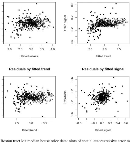
Even if prediction for new data is as yet less well grounded, the partition of spatial model fitted values into trend and signal allows us to use alternative diag-nostic plots. Examples of such plots for the data set discussed in section 4.2 below are shown in Fig. 1. Tracts lying in towns in Boston city are distinguished in the plot, since their patterns seem to indicate different behaviour both in relation to the aspatial trend, and the spatial autoregressive error signal. It may be remarked that the fit of the spatial error model (AIC = -508.85) is better than that of the spatial lag model (AIC = -498.02), than the aspatial linear model (AIC = -283.96), but worse than the mixed spatial lag model (AIC = -545.23). The full results may be obtained by executingexample(boston)after loading spdep intoR, in which the sphere of influence row standardised weighting scheme is also presented.
2.0 2.5 3.0 3.5 4.0
−0.6
−0.2
0.2
0.6
Residuals by fitted values
Fitted values Residuals 2.5 3.0 3.5 −0.6 −0.2 0.2 0.6
Fitted signal by fitted trend
Fitted trend Fitted signal 2.5 3.0 3.5 −0.6 −0.2 0.2 0.6
Residuals by fitted trend
Fitted trend Residuals −0.6 −0.2 0.0 0.2 0.4 0.6 −0.6 −0.2 0.2 0.6
Residuals by fitted signal
Fitted signal
Residuals
Fig. 1 Boston tract log median house price data: plots of spatial autoregressive error model
fit components and residuals for all 506 tracts; tracts in towns in Boston plotted with .
4.2 Boston housing values case
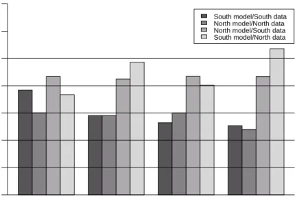
Using the data set described by Gilley and Pace (1996), a revision of the Harrison and Rubinfeld Boston hedonic house price data, relating median house values to a range of environmental and social variables over 506 tracts, we will try two prediction settings. In the first, the data are divided into northern and southern parts at UTM zone 19 northing 4,675,000m (dividing the tracts into two almost equal groups, with the dividing line running through the Boston city tracts). The data frame is subsetted by a logical variable expressing whether the centre point of the tract is north or south of the dividing line. The spatial weights used are constructed using the sphere of influence approach based on a triangulation of the UTM zone 19 projected tract centres, subsetted using the same north/south logical variable. An ordinary least squares model was fitted to each of the parts of the city, and predictions were made with the data used for fitting the models, and then using the model fitted on the southern data with the northern data, and vice-versa. The
Linear Spatial lag Spatial error Spatial mixed South model/South data North model/North data North model/South data South model/North data
Root mean square errors by model and prediction data
Models
Root mean square error
0.00 0.05 0.10 0.15 0.20 0.25 0.30 0.35
Fig. 2 Comparison of model prediction root mean square errors for four models divided
north/south, Boston house price data.
same procedure was repeated for the spatial lag model, the spatial error model, and the spatial mixed model (the spatial lag model augmented with the spatial lags of the explanatory variables).
Although it can be seen from Fig. 2 that the spatial models are better fitted to the data, especially in the south, the cross-predictions are no better than, and often worse than those for the aspatial linear model (lm). The linear model gives the best prediction of the southern median house prices using the fitted coefficient values from the northern data. At least part of the reason for this is that the fits of the models, both aspatial and spatial coefficient values, differed between the two parts of the metropolitan area, suggesting that spatial regimes and/or non-stationarity are present.
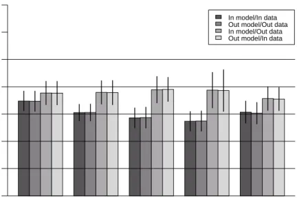
In the second approach, 100 samples of 250 in-sample tracts were chosen, leav-ing 256 tracts out-of-sample. The samples were replicated in order to get a feelleav-ing for the variations in predictions which could result. Here, the spatial weights ma-trices were prepared for each data set as row standardised schemes for the six nearest neighbours of each tract centre (UTM zone 19). In addition, use was made of thegam()function in package mgcv to fit a generalised additive model. In this specification, the model fitted was:
* 7
R"#?
Linear Spatial lag Spatial error Spatial mixed Generalized Additive In model/In data Out model/Out data In model/Out data Out model/In data
Models
Root mean square error
0.00 0.05 0.10 0.15 0.20 0.25 0.30 0.35
RMSE for 100 samples: Mean and 2 standard deviations
Fig. 3 Comparison of model prediction root mean square errors means and standard
devia-tions for 100 random samples of 250 in-sample tracts and 256 out-of-sample tracts, for five models, Boston house price data.
where 7
R #?
is a smoothing function using a penalized thin plate regression spline basis in 12 dimensions to incorporate spatial dependence. Alternative mod-ern statistical fitting techniques could have been used, and here the joint smoothing of longitude and latitude was chosen after inspecting the results of smoothing each of them and their interaction separately. This approach was suggested by the use of geographical coordinates by Wood (2001).
Fig. 3 reinforces the results of testing model predictions after dividing Boston into two parts. The linear model (lm) has the least satisfactory fit within the sam-ple from which the model was fitted, but performs as well or better than all the spatial econometrics models when predicting for other data than those used to fit the model. The mixed spatial lag model does best in predicting on the training set — the data it was fitted with, but worst on the test — excluded — data. This may be taken as an indication of over-fitting, capturing too much of the specificity of the spatial dependencies of the training data set. The performance of the gener-alised additive model is better than that of the linear model both on the training and the test data sets, despite the "black-box" nature of the specification of the spatial dependence in this case as penalized thin plate regression spline.
5 Concluding remarks
Among the opportunities and challenges posed by trying to implement spatial econometric techniques inRin the spdep package have been issues raised by the object-oriented data-driven approach implicit in classes and methods. So far, old style classes and methods have been used for spatial neighbour objects, spatial weights objects, and for spatial simultaneous autoregressive model objects. Many of the methods usually accompanying fitted model objects are simple to write, but predict.sarlm()revealed areas of spatial econometrics which perhaps have received little attention hitherto. The current implementation does however need to be augmented to handle situations in which the dependencies between the lo-cations of observations from which the model to be used for prediction was fitted, and the locations of new data observations, can be represented as a correlation structure of some kind, thus better capturing the signal component.
It does seem that Haining’s partitioning of the fitted values of spatial models is of interest in itself, as indicated by the diagnostic plots in Fig. 1. It may well be that such diagnostic plots, perhaps dynamically linked to maps, will help us in establishing which further misspecification problems are present in our spatial models, shifting focus from criticising the misspecification of aspatial models to trying to construct spatial models with better properties. Haining’s proposals for more general regression diagnostics for models in which spatial dependence is present do not seem to have as yet met with the acceptance they deserve (1990, 1994). Prediction for new data and new spatial weights matrices is a challenge for legacy spatial econometric models, raising the question of what spatial predic-tions should look like. Can for example spatial econometrics models be recast as mixed effects models, since as Pinheiro and Bates (2000) show, spatial correlation structures can “plugged” into such models?
A further consequence of examining fitted model classes and methods, in par-ticular with regard to prediction, is to question whether we need to fit models on very large data sets. Can we not rather fit and refine them on smaller data sets and predict or interpolate to larger data sets? Housing values are not infrequently the subject of analysis, and would perhaps be an attractive target for prediction. An advantage of fitting on moderate sized data sets, maybe training sets from larger data collections, is that the use of sparse matrix techniques in some circumstances would become unnecessary. Standard errors of prediction remain open.
It also seems that a relaxation of single data set fitting of spatial econometrics models may also help to lower barriers between geostatistics and legacy spatial econometrics models when using distance criteria for representing dependence. It appears that some movement is already taking place in this regard, given the use of spatial covariance in Ord and Getis (2001) in the development of the
7:? local spatial autocorrelation statistic allowing for global dependence. In addition, the Getis filtering approach (Getis, 1995, Getis and Griffith, 2002) is distance based, and seems to admit prediction to new data locations using the distance criteria and filtering functions recorded in the fitted model. The Griffith eigenfunction decom-position approach discussed in Getis and Griffith (2002), and described in detail in Griffith (2000a, 2000b), does not, however, seem to open for prediction to new
lo-cations not contiguous with the lolo-cations on which the estimated model was fitted, because of its clear focus on the eigenvectors of the spatial weights matrix of the training data set. In addition, the selection of the eigenvectors to use for filtering may not transfer between geographical settings.
Finally, focusing on prediction using spatial econometric models does concen-trate attention on assumptions about spatial homogeneity, including stationarity, support, multi-scale issues, and edge effects. Approaching modern statistical tech-niques as it were from the other side, we find work on geographically weighted regression (Brunsdon et al. 1996) and geographically weighted summary statis-tics (Brunsdon et al. 2002), in which many of these assumptions are addressed directly. In this context, it would be worthwhile to be able to test a geographically weighted regression fit against say a spatial error model fit, for instance by imple-menting a model comparison function likeanova(gwr.fit, sarlm.fit). But it is the flexibility of a language environment such asR, and the fruitfulness of class and method formalisms, that give rise to such projects for future research and implementation.
References
Anselin L (1988) Spatial econometrics: Methods and models. Kluwer, Dordrecht Anselin L (1995) SpaceStat version 1.80 user’s guide. Morgantown, WV:
Re-gional Research Institute, West Virginia University
Banos A (2001) A propos de l’analyse spatiale exploratoire des données. Cyber-geo4197
Becker RA, Chambers JM, Wilks AR (1988) The New S Language. Chapman & Hall, London
Bennett RJ, Haining RP, Griffith DA (1984) The problem of missing data on spatial surfaces. Annals of the Association of American Geographers 74: 138– 156
Bivand RS (2001a)Rand geographical information systems, especially GRASS. Proceedings of the 2nd International Workshop on Distributed Statistical Com-puting, Technische Universität Wien, Vienna, Austria
Bivand RS (2001b) More on Spatial Data Analysis. R News 1 (3): 13–17 Bivand RS (2002) Implementing spatial data analysis software tools in R.
Un-published paper for CSISS specialist meeting on spatial data analysis software tools, Santa Barbara CA, 10–11 May 2002
Bivand RS, Gebhardt A (2000) Implementing functions for spatial statistical analysis using theRlanguage. Journal of Geographical Systems 2: 307–317 Bivand RS, Portnov BA (forthcoming) Exploring spatial data analysis techniques
usingR: the case of observations with no neighbours. In: Anselin L, Florax R, Rey S (eds) Advances in spatial econometrics, Springer, Berlin, Heidelberg and New York
Brunsdon C, Fotheringham AS, Charlton M (1996) Geographically weighted re-gression: a method for exploring spatial nonstationarity. Geographical Analy-sis 28: 281–289
Brunsdon C, Fotheringham AS, Charlton M (2002) Geographically weighted summary statistics — a framework for localised exploratory data analysis. Computers, Environment and Urban Systems 26: 501–524
Chambers JM (1998) Programming with data. Springer, Berlin, Heidelberg and New York
Chambers JM, Hastie TJ (1992) Statistical models inS. Chapman & Hall, Lon-don
Cliff, AD, Ord JK (1973) Spatial autocorrelation. Pion, London
Cox NJ, Jones K (1981) Exploratory data analysis. In: Wrigley N, Bennett RJ (eds) Quantitative geography: A British view. London, Routledge & Kegan Paul, pp. 135–143
Cressie NAC (1993) Statistics for spatial data. Wiley, New York.
Dalgaard P (2002) Introductory statistics withR. Springer, Berlin, Heidelberg and New York.
Diggle PJ, Tawn JA, Moyeed RA (1998) Model-based geostatistics. Applied Statis-tics 47: 299–350
Getis A (1995) Spatial filtering in a regression framework: Examples using data on urban crime, regional inequality, and government expenditure. In: Anselin L, Florax RJGM (eds) New directions in spatial econometrics. Springer, Berlin, Heidelberg and New York.
Getis A, Griffith DA (2002) Comparative spatial filtering in regression analysis. Geographical Analysis 34: 130–140
Gilley OW, Pace RK (1996) On the Harrison and Rubinfeld data. Journal of Environmental Economics and Management 31: 403–405
Gotway CA, Young LJ (2002) Combining incompatible spatial data. Journal of the American Statistical Association 97: 632–648
Griffith DA (1989) Spatial regression analysis on the PC: Spatial statistics us-ing MINITAB. Discussion Paper, Institute of Mathematical Geography, Ann Arbor, Michigan
Griffith DA (2000a) A linear regression solution to the spatial autocorrelation problem. Journal of Geographical Systems 2: 141–156
Griffith DA (2000b) Eigenfunction properties and approximations of selected in-cidence matrices employed in spatial analyses. Linear Algebra and Its Appli-cations 321: 95–112
Griffith DA, Bennett RJ, Haining RP (1989) Statistical analysis of spatial data in the presence of missing observations — a methodological guide and an appli-cation to urban census data. Environment and Planning A 21: 1511–1523 Griffith DA, Layne LJ (1999) A casebook for spatial statistical Ddata analysis:
A compilation of analyses of different thematic data sets. Oxford University Press, New York.
Gould P (1970) Is Statistix Inferens the geographical name for a wild goose? Economic Geography 46: 439–448
Haining RP (1981) Spatial and temporal analysis: Spatial modelling. In: Wrigley N, Bennett RJ (eds) Quantitative geography: A British view, London, Rout-ledge & Kegan Paul, pp. 86–91
Haining RP (1990) Spatial data analysis in the social and environmental sci-ences. Cambridge University Press, Cambridge
Haining RP (1990) The use of added variable plots in regression modeling with spatial data. Professional Geographer 42: 336–344
Haining RP (1994) Diagnostics for regression modeling in spatial econometrics. Journal of Regional Science 34: 325–341
Haining RP, Griffith DA, Bennett RJ (1989) Maximum-likelihood estimation with missing spatial data and with an application to remotely sensed data. Communications in Statistics — Theory and Methods 18: 1875–1894
Hartwig F, Dearing BE (1979) Exploratory data analysis. Beverly Hills, Sage Ihaka R, Gentleman R (1996) R: A Language for Data Analysis and Graphics.
Journal of Computational and Graphical Statistics 5: 299–314
Johnson J, NiDardo J (1997) Econometric methods. Mc Graw Hill, New York Kaluzny SP, Vega SC, Cardoso TP, Shelly AA (1996) S+SPATIALSTATS users
manual version 1.0. MathSoft Inc., Seattle
Martin RJ (1984) Exact maximum likelihood for incomplete data from a cor-related Gaussian process. Communications in Statistics: Theory and Methods 13: 1275–1288
Martin RJ (1990) The role of spatial statistical processes in geographical mod-elling. In: Griffith DA (ed) Spatial statistics: Past, present, and future, Ann Arbor, Michigan, Institute of Mathematical Geography, pp. 109–127
Olsson, G (1968) Complementary models: A study of colonization maps. Ge-ografiska Annaler B 50: 115–132
Olsson, G (1970) Explanation, prediction, and meaning variance: An assessment of distance interaction models. Economic Geography 46: 223–233
Ord JK, Getis A (2001) Testing for local spatial autocorrelation in the presence of global autocorrelation. Journal of Regional Science 41: 411–432
Pinheiro JC, Bates DM (2000) Mixed-effects models inSandS-PLUS. Springer, Berlin, Heidelberg and New York
Ripley BD (1988) Statistical inference for spatial processes. Cambridge Univer-sity Press, Cambridge
Ripley BD (1992) Applications of Monte-Carlo methods in spatial and image analysis. In: Jöckel KJ, Rothe G, Sendler W (eds) Bootstrapping and related techniques, Springer, Berlin, 47–53
Stewart MB, Wallis KF (1981) Introductory econometrics. Blackwell, Oxford Venables WN, Ripley BD (2000)S programming. Springer, Berlin, Heidelberg
and New York
Venables WN, Ripley BD (2002) Modern applied statistics withS-PLUS. Springer, Berlin, Heidelberg and New York (fourth edition)
Wood SN (2001) mgcv: GAMs and Generalized Ridge Regression forR. R News 1 (2): 20–25