ScholarlyCommons
Statistics Papers
Wharton Faculty Research
2008
Efficient Bandit Algorithms for Online Multiclass
Prediction
Sham M. Kakade
University of Pennsylvania
Shai Shalev-Shwartz
Toyota Technological Institute
Ambuj Tewari
Toyota Technological Institute
Follow this and additional works at:
http://repository.upenn.edu/statistics_papers
Part of the
Statistics and Probability Commons
This paper is posted at ScholarlyCommons.http://repository.upenn.edu/statistics_papers/119 For more information, please [email protected].
Recommended Citation
Kakade, S. M., Shalev-Shwartz, S., & Tewari, A. (2008). Efficient Bandit Algorithms for Online Multiclass Prediction.Proceedings of the 25th International Conference on Machine Learning,440-447. Retrieved fromhttp://repository.upenn.edu/statistics_papers/119
Efficient Bandit Algorithms for Online Multiclass Prediction
Abstract
This paper introduces the Banditron, a variant of the Perceptron [Rosenblatt, 1958], for the multiclass bandit
setting. The multiclass bandit setting models a wide range of practical supervised learning applications where
the learner only receives partial feedback (referred to as "bandit" feedback, in the spirit of multi-armed bandit
models) with respect to the true label (e.g. in many web applications users often only provide positive "click"
feedback which does not necessarily fully disclose a true label). The Banditron has the ability to learn in a
multiclass classification setting with the "bandit" feedback which only reveals whether or not the prediction
made by the algorithm was correct or not (but does not necessarily reveal the true label). We provide
(relative) mistake bounds which show how the Banditron enjoys favorable performance, and our experiments
demonstrate the practicality of the algorithm. Furthermore, this paper pays close attention to the important
special case when the data is linearly separable --- a problem which has been exhaustively studied in the full
information setting yet is novel in the bandit setting.
Keywords
Online learning, Bandit algorithms, Perceptron
DisciplinesStatistics and Probability
Sham M. Kakade [email protected]
Shai Shalev-Shwartz [email protected]
Ambuj Tewari [email protected]
Toyota Technological Institute, 1427 East 60th Street, Chicago, Illinois 60637, USA
Keywords: Online learning, Bandit algorithms, Perceptron
Abstract
This paper introduces the Banditron, a vari-ant of the Perceptron [Rosenblatt, 1958], for the multiclass bandit setting. The multiclass bandit setting models a wide range of prac-tical supervised learning applications where the learner only receives partial feedback (re-ferred to as “bandit” feedback, in the spirit of multi-armed bandit models) with respect to the true label (e.g. in many web applications users often only provide positive “click” feed-back which does not necessarily fully disclose a true label). The Banditron has the abil-ity to learn in a multiclass classification set-ting with the “bandit” feedback which only reveals whether or not the prediction made by the algorithm was correct or not (but does not necessarily reveal the true label). We pro-vide (relative) mistake bounds which show how the Banditron enjoys favorable perfor-mance, and our experiments demonstrate the practicality of the algorithm. Furthermore, this paper pays close attention to the impor-tant special case when the data is linearly separable — a problem which has been ex-haustively studied in the full information set-ting yet is novel in the bandit setset-ting.
1. Introduction
In the conventional supervised learning paradigm, the learner has access to a data set in which the true labels of the inputs are provided. While attendant learning algorithms in this paradigm are enjoying wide ranging
Appearing inProceedings of the 25thInternational
Confer-ence on Machine Learning, Helsinki, Finland, 2008.
Copy-right 2008 by the author(s)/owner(s).
success, their effective application to a number of do-mains, including many web based applications, hinges on being able to learn in settings where the true la-bels are not fully disclosed, but rather the learning algorithm only receives some partial feedback. Impor-tant domains include both the (financially imporImpor-tant) sponsored advertising on webpages and recommender systems. The typical setting is: first, a user queries the system; then using the query and other poten-tially rich knowledge the system has about the user (e.g. past purchases, their browsing history, etc.) the system makes a suggestion (e.g. it presents the user with a few ads they might click on or songs they might buy); finally, the user either positively or negatively re-sponds to the suggestion. Crucially, the system does not learn what would have happened had other sug-gestions been presented.
We view such problems as naturally being online, “bandit” versions of multiclass prediction problems, and, in this paper, we formalize such a model. In essence, this multiclass bandit problem is as follows: at each round, the learner receives an inputx(say the users query, profile, and other high dimensional infor-mation); the learner predicts some class label ˆy (the suggestion); then the learner receives the limited feed-back of only whether the chosen label was correct or not. In the conventional, “full information” supervised learning model, a true labely(possibly more than one or none at all) is revealed to the learner at each round — clearly unrealistic in the aforementioned applica-tions. In both cases, the learner desires to make as few mistakes as possible. The bandit version of this prob-lem is clearly more challenging, since, in addition to the issues ones faces for supervised learning (e.g. learn-ing a mapplearn-ing from a high dimensional input space to the label space), one also faces balancing exploration and exploitation.
spaces, namely linear predictors, in the bandit setting. Somewhat surprisingly, while there has been a stag-gering number of results on (margin based) linear pre-dictors and much recent work on bandit models, the intersection of these two settings is novel and opens a number of interesting (both theoretical and practical) questions, which we consider. In particular, we pay close attention to the important case where the data are linearly separable, where, in the full information setting, the (efficient) Perceptron algorithm makes a number of mistakes that is asymptotically bounded (so the actual error rate will rapidly converge to 0). There are a number of related results in the bandit literature. The Exp4 algorithm (for the “experts” set-ting) of Auer et al. [1998] and the contextual bandit setting of Langford and Zhang [2007] are both bandit settings where the learner has side information (e.g. the input “x”) when making a decision — in fact, our setting can be thought of as a special case of the con-textual bandit setting1. However, these settings
con-sider abstract hypothesis spaces and do not explicitly consider efficient algorithms. Technically related are the bandit algorithms for online convex optimization of Flaxman et al. [2005], Kleinberg [2004], which at-tempt to estimate a gradient (for optimization) with only partial feedback. However, these algorithms do not apply due to the subtleties of using the non-convex classification loss, which we discuss at the end of Sec-tion 2.
This paper provides an efficient bandit algorithm, the Banditron, for multiclass prediction using linear hypothesis spaces, which enjoys a favorable mistake bound. We provide empirical results showing our al-gorithm is quite practical. For the case where the data is linearly separable, our mistake bound isO(√T) inT
rounds. We also provide results toward characterizing the optimal achievable mistake bound for the linearly separable case (ignoring efficiency issues here) and in-troduce some important open questions regarding this issue. In the Extensions section, we also discuss up-date rules which generalize the Winnow algorithm (for L1 margins) and margin-mistake based algorithms to the bandit setting. We also discuss how our algorithm can be extended to ranking and settings where more than one prediction ˆy can be presented to the user (e.g. an advertising setting where multiple ads may be presented).
1
The contextual bandit setting can be thought of as a general cost sensitive classification problem with bandit feedback. While their setting is an i.i.d. one, we make no statistical assumptions.
2. Problem Setting
We now formally define the problem of online multi-class prediction in the bandit setting. Online learning is performed in a sequence of consecutive rounds. On roundt, the learner is given an instance vectorxt∈Rd
and is required to predict a label out of a set ofk pre-defined labels which we denote by [k] = {1, . . . , k}. We denote the predicted label by ˆyt. In the full in-formation case, after predicting the label, the learner receives the correct label associated with xt, which we denote by yt ∈ [k]. We consider a bandit set-ting, in which the feedback received by the learner is
1[ˆyt6=yt], where 1[π] is 1 if predicate π holds and 0 otherwise. That is, the learner knows if it predicted an incorrect label, but it does not know the identity of the correct label. The learner’s ultimate goal is to mini-mize the number of prediction mistakes,M, it makes along its run, where:
M = T X t=1
1[ˆyt6=yt] .
To make M small, the learner may update its pre-diction mechanism after each round so as to be more accurate in later rounds.
The prediction of the algorithm at round t is deter-mined by a hypothesis, ht : Rd → [k], where ht is taken from a class of hypotheses H. In this paper we focus on the class of margin based linear hypotheses. Formally, eachh∈ His parameterized by a matrix of weightsW ∈Rk×d and is defined to be:
h(x) = argmax j∈[k]
(Wx)j , (1)
where (Wx)jis thejth element of the vector obtained by multiplying the matrixW with the vectorx. Since each hypothesis is parameterized by a weight matrix, we refer to a matrix W also as a hypothesis — by that we mean that the prediction is defined as given in Eq. (1). To evaluate the performance of a weight matrix W on an example (x, y) we check whether
W makes a prediction mistake, namely determine if arg maxj(Wx)j6=y.
The class of margin based linear hypotheses for mul-ticlass learning has been extensively studied in the full information case [Duda and Hart, 1973, Vapnik, 1998, Weston and Watkins, 1999, Elisseeff and We-ston, 2001, Crammer and Singer, 2003]. Our start-ing point is a simple adaptation of the Perceptron algorithm [Rosenblatt, 1958] for multiclass prediction in the full information case (this adaptation is called Kesler’s construction in [Duda and Hart, 1973, Cram-mer and Singer, 2003]). Despite its age and simplicity,
the Perceptron has proven to be quite effective in prac-tical problems, even when compared to state-of-the-art large margin algorithms [Freund and Schapire, 1999]. We denote byWtthe weight matrix used by the Per-ceptron at roundt. The Perceptron starts with the all zero matrixW1=0and updates it as follows
Wt+1 = Wt+Ut , (2) whereUt∈
Rk×d is the matrix defined by
Ur,jt = xt,j(1[yt=r]−1[ˆyt=r]). (3) In other words, if there is no prediction mistake (i.e.
yt = ˆyt), then there is no update (i.e. Wt+1 =Wt), and if there is a prediction mistake, then xt is added to the ytth row of the weight matrix and subtracted from the ˆytth row of the matrix.
A relative mistake bound can be proven for the mul-ticlass Perceptron algorithm. The difficulty with pro-viding mistake bounds for any (efficient) algorithm in this setting stems from the fact that the classification loss is non-convex. Hence, performance bounds are commonly evaluated using the multiclasshinge-loss— what might be thought of as a convex relaxation of the classification loss. In particular, the hinge-loss of W
on (x, y) is defined as follows:
`(W; (x, y)) = max
r∈[k]\{y}[1−(Wx)y+ (Wx)r]+ ,
(4) where [a]+ = max{a,0} is the hinge function. The hinge-loss will be zero only if (Wx)y−(Wx)r≥1 for all r6=y. The difference (Wx)y−(Wx)r is a gener-alization of the notion of margin from binary classifi-cation. Let ˆy = argmaxr(Wx)r be the prediction of
W. Note that if ˆy 6= y then `(W; (x, y))≥1. Thus, the hinge-loss is a convex upper bound on the zero-one loss function,`(w; (x, y))≥1[ˆy6=y].
The Perceptron mistake bound holds for any sequence of examples and compares the number of mistakes made by the Perceptron with the cumulative hinge-loss of any fixed weight matrixW?, even one defined with prior knowledge of the sequence. Formally, let (x1, y1), . . . ,(xT, yT) be a sequence of examples and assume for simplicity that kxtk ≤1 for allt. LetW? be any fixed weight matrix. We denote by
L= T X t=1
`(W?; (xt, yt)) , (5)
the cumulative hinge-loss ofW? over the sequence of examples and by D= 2kW?k2F = 2 k X r=1 d X j=1 (Wi,j? ) 2 , (6)
Algorithm 1The Banditron
Parameters: γ∈(0,0.5) InitializeW1=0∈
Rk×d
fort= 1,2, . . . , T do
Receivext∈Rd
Set ˆyt= arg maxr∈[k](Wtxt)r
∀r∈[k] defineP(r) = (1−γ)1[r= ˆyt] +γk Randomly sample ˜yt according toP Predict ˜ytand receive feedback1[˜yt=yt] Define ˜Ut∈ Rk×d such that: ˜ Ut r,j=xt,j 1[y t=˜yt]1[˜yt=r] P(r) −1[ˆyt=r] Update: Wt+1=Wt+ ˜Ut end for
thecomplexity ofW?. Herek · k2
F denotes the Frobe-nius norm. Then the number of prediction mistakes of the multiclass Perceptron is at most,
M ≤ L+D+√L D . (7) A proof of the above mistake bound can be found for example in Fink et al. [2006]. The mistake bound in Eq. (7) consists of three terms: the loss of W?, the complexity ofW?, and a sub-linear term which is often negligible. In particular, when the data is separable (i.e. L= 0), the number of mistakes is bounded byD.
Unfortunately, the Perceptron’s update cannot be im-plemented in the bandit setting as we do not know the identity of yt. One direction is to work directly with the hinge-loss (which is convex) and try to use the ban-dit algorithms for online convex optimization of Flax-man et al. [2005], Kleinberg [2004]. In this work, they attempt to find an unbiased estimate of the gradient using only bandit feedback (i.e. using only the loss re-ceived as feedback). However, since the only feedback the learner receives is 1[ˆyt6=yt], one does not neces-sarily even know the hinge-loss for the chosen decision, ˆ
yt, due to dependence of the hinge loss on the true la-bel yt. Hence, the results of Flaxman et al. [2005], Kleinberg [2004] are not directly applicable.
3. The Banditron
We now present the Banditron in Algorithm 1, which is an adaptation of the multiclass Perceptron for the bandit case.
Similar to the Perceptron, at each round we let ˆyt be the best label according to the current weight matrix
Wt, i.e. ˆy
t= argmaxr(Wtxt)r. Most of the time the Banditron exploits the quality of the current weight matrix by predicting the label ˆyt. Unlike the Percep-tron, if ˆyt6=yt, then we can not make an update since we are blind to the identity ofyt. Roughly speaking,
it is difficult to learn when we exploit usingWt. For this reason, on some of the rounds we let the algo-rithm explore (with probability 1−γ) and uniformly predict a random label from [k]. We denote by ˜ytthe predicted label. On rounds in which we explore, (so ˜
yt6= ˆyt), if we additionally receive a positive feedback, i.e. ˜yt=yt, then we indirectly obtain the full informa-tion regarding the identity ofyt, and we can therefore update our weight matrix using this positive instance. The parameterγcontrols the exploration-exploitation tradeoff.
The above intuitive argument is formalized by defining the update matrix ˜Utto be a function of the random-ized prediction ˜yt. We emphasize that ˜Utaccesses the correct label yt only through the indicator 1[yt= ˜yt] and is thus adequate for the Bandit setting. As we show later in Lemma 4, the expected value of the Banditron’s update matrix ˜Ut is exactly the Percep-tron’s update matrix Ut. While there a number of other variants which also perform unbiased updates, we have found this one provides the most favorable performance (empirically speaking).
The following theorem provides a bound on the ex-pected number of mistakes the Banditron makes.
Theorem 1. (Mistake Bound). Assume that for the
sequence of examples, (x1, y1), . . . ,(xT, yT), we have,
for all t,xt∈Rd,kxtk ≤1, and yt∈[k]. LetW? be
any matrix, letLbe the cumulative hinge-loss ofW?as
defined in Eq. (5), and let D be the complexity ofW?
(i.e. D= 2||W?||2
F). Then the number of mistakes M
made by the Banditron satisfies
E[M] ≤ L+γ T+ 3 max n k D γ , p D γ To+qk D L γ .
where expectation is taken with respect to the random-ness of the algorithm.
Before turning to the proof of Thm. 1 let us first opti-mize the exploration-exploitation parameter γ in dif-ferent scenarios. First, assume that the data is sepa-rable, that isL= 0. In this case, we can obtain a mis-take bound of O(√T). In fact the following corollary shows that an O(√T) bound is achievable whenever the cumulative hinge-loss ofW? is small enough.
Corollary 2(Low noise). Assume that the conditions
stated in Thm. 1 hold and that there exists W? with
fixed complexity D and loss L ≤ O(√D k T). Then, by setting γ =pk D/T we obtain the bound E[M] ≤
O(√k D T).
Next, let us consider the case where we have a constant (average) noise level of ρ, i.e. there exists ρ ∈ (0,1) such thatL≤ρT. In this case,
Corollary 3(High noise). Assume that the conditions
stated in Thm. 1 hold and that there exists W? with
fixed complexityD and lossL≤ρ T for a constantρ∈
(0,1). Then, by settingγ=ρ(k D/T)1/3we obtain the
boundE[M]≤ρT(1+)where=O((k D)1/3T−1/3).
We note that the bound in the above corollary can be also written in an additive form as: E[M]−L ≤
O(T2/3). However, since we are not giving proper
re-gret bounds as we compare mistakes to hinge-loss we prefer to directly boundE[M].
Analysis: To prove Thm. 1 we first show that the
random matrix ˜Utis an unbiased estimator of the up-date matrix Ut used by the Perceptron. Formally, letEt[ ˜Ut] be the expected value of ˜Ut conditioned on ˜
y1, . . . ,y˜t−1. Then:
Lemma 4. Let U˜t be as defined in Algorithm 1 and
letUt be as defined in Eq. (3). Then,Et[ ˜Ut] =Ut.
Proof. For eachr∈[k] andj ∈[d] we have
Et[ ˜Ur,jt ] = k X i=1 P(i)xt,j 1[i=y t]1[i=r] P(r) −1[ˆyt=r] = xt,j(1[yt=r]−1[ˆyt=r]) = Ur,jt , which completes the proof.
Next, we bound the expected squared norm of ˜Ut.
Lemma 5. LetU˜tbe as defined in Algorithm 1. Then,
Et[kU˜tkF2 ]≤2kxtk2 k γ 1[yt6= ˆyt] +γ1[yt= ˆyt] .
Proof. We first observe that
kU˜tk2 F = kxtk2 1 P(yt)2 + 1 if ˜yt=yt6= ˆyt kxtk2 1 P(yt)−1 2 if ˜yt=yt= ˆyt kxtk2 if ˜yt6=yt Therefore, ifyt6= ˆytthen Et[kU˜tk2F] kxtk2 = P(yt) 1 P(yt)2 + 1 + (1−P(yt)) = 1 +P(1y t) = 1 + k γ ≤ 2k γ , and ifyt= ˆytthen Et[kU˜tk2F] kxtk2 = P(yt) 1 P(yt)−1 2 + (1−P(yt)) = P(1y t)−1≤ 1 1−γ −1≤ γ 1−γ ≤2γ . Combining the two cases concludes our proof.
Equipped with the above two lemmas, we are ready to prove Thm. 1.
Proof of Thm. 1. Throughout the proof we use the notation hW?, Wti := Pk r=1 Pd j=1W ? r,jWr,jt . We prove the theorem by bounding E[hW?, WT+1i] from
above and from below starting with a lower bound. We can first use the fact that W1 = 0 to rewrite
E[hW?, WT+1i] as PTt=1∆twhere
∆t:=E[hW?, Wt+1i]−E[hW?, Wti] .
Expanding the definition ofWt+1 and using Lemma 4
we obtain that for all t, ∆t = E[hW?,U˜ti] = E[hW?, Uti].Next, we note that the definition of the
hinge-loss given in Eq. (4) implies that the following holds regardless of the value of ˆyt
`(W?,(xt, yt)) ≥ 1[ˆyt6=yt]− hW?, Uti . Therefore ∆t ≥ E[1[ˆyt6=yt] ]−`(W?,(xt, yt)) . Sum-ming over twe obtain the lower bound
E[hW?, WT+1i] =
T X t=1
∆t ≥ E[ ˆM]−L , (8)
where Mˆ := PTt=1 1[ˆyt6=yt] and L is as de-fined in Eq. (5). Next, we show an upper bound on E[hW?, WT+1i]. Using Cauchy-Schwartz
inequal-ity we have hW?, WT+1i ≤ kW?k
FkWT+1kF . To ease our notation, we use the shorthand k · k for de-noting the Frobenius norm. Using the definition ofD
given in Eq. (6), the concavity of the sqrt function, and Jensen’s inequality we obtain that
E[hW?, WT+1i]≤
q
DE[kWT+1k2]
2 . (9)
We therefore need to upper bound the expected value of kWT+1k2. Expanding the definition of WT+1 we
get that E[kWT+1k2] = E[kWTk2+hWT,U˜Ti+kU˜Tk2] = T X t=1 E[hWt,U˜ti] +E[kU˜tk2] .
Using Lemma 4 we obtain that E[hWt,U˜ti] =
E[hWt, Uti] ≤ 0, where the second inequality follows
from the definition ofUtand ˆy
t. Combining this with Lemma 5 and with the assumption kxtk ≤1 for all t we obtain that E[kWT+1k2] ≤ T X t=1 E 2k γ 1[yt6= ˆyt] + 2γ1[yt= ˆyt] ≤ 2k γ E[ ˆM] + 2γ T .
Plugging the above into Eq. (9) and using the inequal-ity √a+b≤√a+√bwe get the upper bound
E[hW?, WT+1i]≤ r D kE[ ˆM] γ + p D γ T .
Comparing the above upper bound with the lower bound given in Eq. (8) and rearranging terms yield
E[ ˆM]− r D kE[ ˆM] γ − L+pD γ T≤0.
Standard algebraic manipulations give the bound
E[ ˆM] ≤ L+ q D k L γ + 3 max n D k γ , p D γ To .
Finally, our proof is concluded by noting that in ex-pectation we are exploring no more than γT of the rounds and thusE[M]≤E[ ˆM] +γT.
4. Mistake Bounds Under Separability
In this section we present results towards characteriz-ing the optimal achievable rate for the case where the data is separable. Here, in the full-information set-ting, the mistake bound of the Perceptron algorithm is finite and bounded byD. We now present an (inef-ficient) algorithm showing that the achievable mistake bound in the bandit setting is also finite — thus the Banditron’s mistake bound of O(√T) leaves signifi-cant room for improvement (though the algorithm is quite simple and has reasonable performance, which we demonstrate in the next section).
First, as a technical tool, we make the interesting ob-servation that the halving algorithm (generalized to the multiclass setting) is also applicable to the bandit setting. The algorithm is as follows: LetH0be the
cur-rent set of “active” experts, which is initialized to the full set, i.e. H=H0att= 1. At each roundt, we
pre-dict using the majority prepre-dictionr(i.e. the prediction
r ∈[k] which the most hypotheses in H0 predict). If
we are correct, we make no update. If we are incorrect, we remove from the active set,H0, thoseh∈ H0which
predicted the incorrect labelr. Crucially, this (gener-alized) halving algorithm is implementable with only the bandit feedback that we receive. This algorithm enjoys the following mistake bound.
Lemma 6. (Halving Algorithm). The halving
algo-rithm (in the bandit setting) makes at most kln|H|
mistakes on any sequence in which there exists some hypothesis in Hwhich makes no mistakes.
Proof. Whenever the algorithm makes a mistake, the size of active set is reduced by at least a 1−1/k
fraction, since majority prediction uses a fraction of hypothesis (from the active set) that is at least 1/k. Since the algorithm never removes a perfect hypothesis from the active set, the maximal number of mistakes,
M, that can occur until H0 consists of only perfect
hypotheses satisfies (1−1/k)M|H| ≥1. Using the in-equality (1−1/k)≤e−1/k and solving forM leads to the claim.
Using this, the following theorem shows that the achievable bound for the number of mistakes is asymp-totically finite. Unfortunately, the result has a dimen-sionality dependence on d. The algorithm essentially uses the margin condition to construct an appropri-ately sized cover forH, the set of all linear hypotheses, and runs the halving algorithm on this cover.
Theorem 7. There exists a deterministic algorithm
(in the bandit setting), taking D as input, which makes at most O(k2dln(Dd)) mistakes on any
se-quence (where kxtk ≤1) that is linearly separable at
margin 1 by someW?, with 2||W?||2
F ≤D.
Proof. (sketch) Since the margin is 1, it is straightfor-ward to show that ifW is a perturbation ofW?which satisfies ||W?−W||
∞ ≤O(√1d), then the data is still
linearly separable under W. By noting that each co-ordinate in W? is (rather crudely) bounded by √D, there exists a discretized grid of Hof sizeO(√Dd)kd which contains a linear separator. The algorithm sim-ply runs the halving algorithm on this cover.
This result is in stark contrast to the Perceptron mis-take bound which has no dependence on the dimen-siond. We now provide a mistake bound with no de-pendence on the dimension. Unfortunately, it is not asymptotically finite, as it is has a rather mild de-pendence on the time — it is O(DlnT) (ignoring k
and higher order terms), while the Perceptron mistake bound isO(D).
Theorem 8. There exists a randomized algorithm (in
the bandit setting), taking as inputs D, T andδ >0, such that with probability greater than 1−δ the algo-rithm makes at most O(k2DlnT+k
δ (lnD+ ln ln T+k
δ ))
mistakes on any T length sequence (where kxtk ≤ 1)
that is linearly separable at margin1by someW?, with 2||W?||2
F ≤D.
The algorithm first constructs a random projection op-erator which projects anyxinto a space of dimension
d0 = O(DlnT+k
δ ), and then it runs the previous al-gorithm in this lower dimensional space. The proof essentially consists of using the results in Arriaga and Vempala [2006] to argue that the (multiclass) margin is preserved under this random projection.
Proof. (sketch) It is simpler to rescale W? such that
||W?||
F = 1 and the margin is 1/
√
D. Consider the
T+kpointsx1toxT and the (row) vectorsW1?, . . . Wk?, whose norms are all bounded by 1. LetP be a matrix of dimension d0 ×d, where each entry of P is inde-pendently sampled fromU(−1,1). Define the projec-tion operator Π(v) = √1
d0P v. Corollary 2 of Arriaga and Vempala [2006] (essentially a result from the JL lemma) shows that ifd0=O(DlnT+δk) then this pro-jection additively preserves the inner products of these points up to 1
3√D, i.e. |Π(W ?
r)·Π(xt)−Wr?·xt| ≤ 3√1D. It follows that, after the projection, the data is lin-early separable with margin at least 1
3√D. Letting Π(W?) denote the matrix where each row of W? has been projected, then, also by the JL lemma, the norm
||Π(W?)||
F will (rather crudely) be bounded by 2 (re-call||W?||
F = 1). Hence, the projected data is linearly separable at margin 1/(3√D) by a weight matrix that has norm O(1), which is identical to being separable at margin 1 with weight vector of complexity O(D). The algorithm is to first create a random projection matrix (which can be constructed without knowledge of the sequence) and then we can run the previous algorithm on the lower dimensional space d0. Since
we have shown that the margin is preserved (up to a constant) in the lower dimensional space, the result follows from the previous Theorem 7, with d0 as the dimensionality.
We discuss open questions in the Extensions section.
5. Experiments
In this section, we report some experimental results for the Banditron algorithm on synthetic and real world data sets. For each data set, we ran Banditron for a wide range of values of the exploration parameter
γ. For each value of γ, we report the average error rate, where the averaging is over 10 independent runs of Banditron.
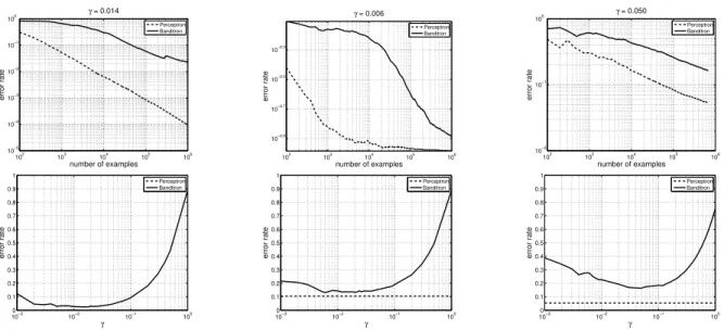
The results are shown on Fig. 1. Each column corre-sponds to one data set. The top figures plot the error rates of Banditron (for the best value of γ) and Per-ceptron as a function of the number of examples seen. We show these on a log-log scale to get a better visual indication of the asymptotics of these algorithms. The bottom figures plot the final error rates on the com-plete data set as a function ofγ. As expected, setting
γ too low or too high leads to higher error rates.
The first data set, denoted by SynSep, is a 9-class, 400-dimensional synthetic data set of size 106. The
102 103 104 105 106 10−5 10−4 10−3 10−2 10−1 100 γ = 0.014 number of examples error rate Perceptron Banditron 102 103 104 105 106 10−0.9 10−0.7 10−0.5 10−0.3 γ = 0.006 number of examples error rate Perceptron Banditron 102 103 104 105 106 10−2 10−1 100 γ = 0.050 number of examples error rate Perceptron Banditron 100−3 10−2 10−1 100 0.1 0.2 0.3 0.4 0.5 0.6 0.7 0.8 0.9 1 γ error rate Perceptron Banditron 100−3 10−2 10−1 100 0.1 0.2 0.3 0.4 0.5 0.6 0.7 0.8 0.9 1 γ error rate Perceptron Banditron 100−3 10−2 10−1 100 0.1 0.2 0.3 0.4 0.5 0.6 0.7 0.8 0.9 1 γ error rate Perceptron Banditron
Figure 1.Error rates of Perceptron (dashed) and Banditron (solid) on the SynSep (left), SynNonSep (middle), and
Reuters4(right) data sets. The 9-class synthetic data sets are generated as follows. We fix 9 bit-vectorsv1, . . . , v9 ∈
{0,1}400 each of which has 20 to 40 bits turned on in its first 120 coordinates. The supports of some of these vectors
overlap. The vectorsvicorrespond to 9 topics where topicihas “keywords” that correspond to the bits turned on invi. To generate an example, we randomly choose aviand randomly turn off 5 bits in its support. Further, we randomly turn on 20 additional bits in the last 280 coordinates. The last 280 coordinates thus correspond to common words that can appear in a document from any topic.
document. The coordinates represent different words in a small vocabulary of size 400. See the caption of Figure 1 for details. We ensure, by construction, that SynSepis linearly separable. The left plots in Figure 1 show the results for this data set. Since this is a sep-arable data set, Perceptron makes a bounded number of mistakes and its error rate plot falls at a rate of 1/T
yielding a slope of −1 on a log-log plot. Corollary 2 predicts that error rate for Banditron should decay faster than 1/√T and we indeed see a slope of approx-imately −0.55 on the log-log plot. The second data set, denoted by SynNonSep, is constructed in the same way asSynSepexcept that we introduce 5% la-bel noise. This makes the data set non-separable. The middle plots in Fig. 1 show the results for SynNon-Sep. The Perceptron error rate decays till it drops to 10% and then becomes constant. Banditron does not decay appreciably till 104 examples after which it falls
rapidly to its final value of 10−0.89= 13%.
We construct our third data set Reuters4from the Reuters RCV1 collection. Documents in the Reuters data set can have more than one label. We restrict ourselves to those documents that have exactly one label from the following set of labels: {ccat, ecat,
gcat, mcat}. This gives us a 4-class data set of size 673,768 which includes about 84% of the documents in the original Reuters data set. We do this because the model considered in this paper assumes that
ev-ery instance has a single true label. See the Extensions section for a discussion about dealing with multiple la-bels. We represent each document using bag-of-words, which leads to 346,810 dimensions. The right plots in Fig. 1 show the results for Reuters4. The final er-ror rates for Perceptron and Banditron (γ= 0.05) are 5.3% and 16.3% respectively. However, it is clear from the top plot that as the number of examples grows, the error rate of Banditron is dropping at a rate com-parable to that of Perceptron.
6. Extensions and Open Problems
We now discuss a few extensions of the Banditron algo-rithm and some open problems. These extensions may possibly improve the performance of the algorithm and also broaden the set of applications that can be tack-led by our approach. Due space constraints, we confine ourselves to a rather high level overview.
Label Ranking: So far we assumed that each
in-stance vector is associated with asingle correct label and we must correctly predict this particular label. In many applications this binary dichotomy is inadequate as each label is associated with a degree of relevance, which reflects to what extent it is relevant to the in-stance vector in hand. Furthermore, it is sometime natural to predict a subset of the labels rather than a single label. For example, consider again the
prob-lem of sponsored advertising on webpages described in the Introduction. Here, the system presents the user with a few ads. If the user positively responds to one of the suggestions (say by a “click”), this implies that the user prefers this suggestion over the other sugges-tions, but it does not necessarily mean that the other suggestions are completely wrong.
We now briefly discuss a possible extension of the Ban-ditron algorithm for this case (using techniques from Crammer et al. [2006]). On each round, we first find thertop ranked labels (where ranking is according to
hwr,xti). With probability 1−γwe exploit and pre-dict these labels. With probability γ we explore and randomly change one of the top ranked labels with another label which is ranked lower by our model. If we are exploring and the user chooses the replaced la-bel, then we obtain a feedback that can be used for improving our model. The Banditron analysis can be generalized to this case, leading to bounds on the num-ber of rounds in which the user negatively responds to our advertisement system.
Multiplicative Updates and Margin-Based
Up-dates: While deriving the Banditron algorithm, our
starting point was the Perceptron, which is an ex-tremely simple online learning algorithm for the full information case. Over the years, many improvements of the Perceptron were suggested (see for example Shalev-Shwartz and Singer [2007] and the references therein). It is therefore interesting to study which al-gorithms can be adapted to the Bandit setting. We conjecture that it is relatively straightforward to adapt the multiplicative update scheme [Littlestone, 1988, Kivinen and Warmuth, 1997] to the bandit setting while achieving mistake bounds similar to the mistake bounds we derived for the Banditron. It is also possi-ble to adapt margin-based updates (i.e. updating also when there is no prediction mistake but only a mar-gin violation) to the bandit setting. Here, however, it seems that the resulting mistake bounds for the low noise case are inferior to the bound we obtained for the Banditron.
Achievable Rates and Open Problems: The
im-mediate question is how to improve our rate ofO(T2/3)
to O(√T) in the general setting with an efficient al-gorithm. We conjecture this is at least possible by some (possibly inefficient) algorithm. Important open questions in the separable case are: What is the opti-mal mistake bound? In particular, does there exist a finite mistake bound which has no dimensionality de-pendence? Furthermore, are there efficient algorithms which achieve the mistake bound of O(DlnT), pro-vided in Theorem 8 (or better)? Practically speaking,
this last question is of the most importance, as then we would have an algorithm that actually achieves a very small mistake bound in certain cases.
References
R.I. Arriaga and S. Vempala. An algorithmic theory of learning: Robust concepts and random projection.
Mach. Learn., 63(2), 2006.
P. Auer, N. Cesa-Bianchi, Y. Freund, and R. E. Schapire. Gambling in a rigged casino: the adversarial multi-armed bandit problem. InProceedings of the 36th
An-nual FOCS, 1998.
K. Crammer and Y. Singer. Ultraconservative online al-gorithms for multiclass problems. Journal of Machine
Learning Research, 3:951–991, 2003.
K. Crammer, O. Dekel, J. Keshet, S. Shalev-Shwartz, and Y. Singer. Online passive aggressive algorithms.Journal
of Machine Learning Research, 7:551–585, Mar 2006.
R. O. Duda and P. E. Hart. Pattern Classification and
Scene Analysis. Wiley, 1973.
A. Elisseeff and J. Weston. A kernel method for multi-labeled classification. InAdvances in Neural Information
Processing Systems 14, 2001.
M. Fink, S. Shalev-Shwartz, Y. Singer, and S. Ullman. On-line multiclass learning by interclass hypothesis sharing.
InProceedings of the 23rd International Conference on
Machine Learning, 2006.
A. Flaxman, A. Kalai, and H. B. McMahan. Online con-vex optimization in the bandit setting: gradient descent without a gradient. InProceedings of the Sixteenth
An-nual ACM-SIAM Symposium on Discrete Algorithms,
pages 385–394, 2005.
Y. Freund and R. E. Schapire. Large margin classification using the perceptron algorithm. Machine Learning, 37 (3):277–296, 1999.
J. Kivinen and M. Warmuth. Exponentiated gradient ver-sus gradient descent for linear predictors. Information
and Computation, 132(1):1–64, January 1997.
R.D. Kleinberg. Nearly tight bounds for the continuum-armed bandit problem. NIPS, 2004.
J. Langford and T. Zhang. The epoch-greedy algorithm for contextual multi-armed bandits. NIPS, 2007.
N. Littlestone. Learning quickly when irrelevant attributes abound: A new linear-threshold algorithm. Machine
Learning, 2:285–318, 1988.
F. Rosenblatt. The perceptron: A probabilistic model for information storage and organization in the brain.
Psy-chological Review, 65:386–407, 1958. (Reprinted in
Neu-rocomputing(MIT Press, 1988).).
S. Shalev-Shwartz and Y. Singer. A primal-dual perspec-tive of online learning algorithms. Machine Learning
Journal, 2007.
V. N. Vapnik. Statistical Learning Theory. Wiley, 1998. J. Weston and C. Watkins. Support vector machines for
multi-class pattern recognition. In Proceedings of the Seventh European Symposium on Artificial Neural