Transductive transfer learning for computer vision.

for

Computer Vision

Dr. Nazli Farajidavar

July 2015

for

Computer Vision

Nazli Farajidavar

Submitted for the Degree of

Doctor of Philosophy

from the

University of Surrey

Centre for Vision, Speech and Signal Processing

Faculty of Engineering and Physical Sciences

University of Surrey

Guildford, Surrey GU2 7XH, U.K.

July 2015

© Nazli Farajidavar 2015

Artificial intelligent and machine learning technologies have already achieved significant

suc-cess in classification, regression and clustering. However, many machine learning methods

work well only under a common assumption that training and test data are drawn from the

same feature space and the same distribution. A real-world applications is in sports footage,

where an intelligent system has been designed and trained to detect score-changing events in

a Tennis single match and we are interested to transfer this learning to either Tennis doubles

game or even a more challenging domain such as Badminton. In such distribution changes,

most statistical models need to be rebuilt, using newly collected training data. In many real

world applications, it is expensive or even impossible to collect the required training data and

rebuild the models. One of the ultimate goals of the open ended learning systems is to take

ad-vantage of previous experience/ knowledge in dealing with similar future problems. Two levels

of learning can be identified in such scenarios. One draws on the data by capturing the pattern

and regularities which enables reliable predictions on new samples. The other starts from an

acquired source of knowledge and focuses on how to generalise it to a new target concept; this

is also known as

transfer learning

which is going to be the main focus of this thesis. This

work is devoted to a second level of learning by focusing on how to transfer information from

previous learnings, exploiting it on a new learning problem with not supervisory information

available for new target data. We propose several solutions to such tasks by leveraging over

prior models or features.

In the first part of the thesis we show how to estimate reliable transformations from the source

domain to the target domain with the aim of reducing the dissimilarities between the source

class-conditional distribution and a new unlabelled target distribution. We then later present a

fully automated transfer learning framework which approaches the problem by combining four

types of adaptation: a projection to lower dimensional space that is shared between the two

domains, a set of local transformations to further increase the domain similarity, a classifier

parameter adaptation method which modifies the learner for the new domain and a set of

class-We conduct experiments on a wide range of image and video classification tasks. class-We test our

proposed methods and show that, in all cases, leveraging knowledge from a related domain can

improve performance when there are no labels available for direct training on the new target

data.

Key words:

Machine Learning, Classification, Transfer Learning, Domain Adaptation.

Email:

[email protected]

WWW: http://www.surrey.ac.uk/cvssp

Foremost, I would like to express my sincere gratitude to my advisors Dr. Teofilo deCampos

and Prof. Josef Kittler for the continuous support of my Ph.D study and research, for their

patience, motivation, enthusiasm, and immense knowledge. Their guidance helped me in all

the time of research and writing of this thesis. I could not have imagined having better advisors

and mentors for my Ph.D study.

Besides my advisor, I would like to thank the rest of my thesis committee: Dr. Timothy

Hospedales, Dr. Janko Calic, Dr. Walterio Mayol-Cuevas and Dr. Terry Windeatt for their

encouragement, insightful comments, and helpful questions.

My sincere thanks also goes to Dr. John Collomosse for offering me a research opportunity in

his group and guiding my work on his project.

I thank my fellow labmates in the Center for Vision, Speach and Signal Processing Group: Dr.

Chi Ho Chan, Dr. Paul Koppen, Dr. Cemre Zor and Dr. Pouria Mortazavian for stimulating

discussions and for all the fun we have had in the last four years.

Last but not the least, I would like to thank my family: my partner Dr. Luca Remaggi, my

parents Vida Khalilian and Dr. Mansour Farajidavar and my beloved brother Dr. Armin

Fara-jidavar for supporting me spiritually throughout my life.

1 Introduction

1

1.1 Problem: Transfer Learning for Computer Vision . . . .

3

1.2 Contributions . . . .

6

1.3 Outline . . . .

8

1.4 List of Publications . . . .

8

2 Background

11

2.1 Notation . . . 13

2.2 Feature Extraction Methods for Image and Video in Computer Vision . . . 14

2.2.1 Histograms of Oriented Gradients in 3D Space-time Blocks (HOG3D) . 15

2.2.2 Bag of Visual Words . . . 17

2.2.3 Deep Convolutional Activation Feature (DeCAF) . . . 17

2.3 Feature Selection . . . 20

2.3.1 Principal Component Analysis . . . 21

2.3.2 Linear Discriminant Analysis . . . 22

2.4 Classification . . . 24

2.4.1 Nearest Neighbor . . . 24

2.4.2 Logistic Regression . . . 25

2.4.3 Support Vector Machines (SVM) . . . 26

2.4.4 Gaussian Classifier . . . 29

2.4.5 Kernel Discriminant Analysis . . . 30

2.5 Transfer Learning . . . 31

2.5.1 Inductive Transfer Learning . . . 33

2.5.2 Transductive Transfer Learning . . . 37

2.5.3 Unsupervised Transfer Learning . . . 43

2.6 Summary . . . 43

3 Databases

45

3.1 ACASVA: Player Actions Database . . . 46

3.1.1 ACASVA System . . . 46

3.1.2 Player Action Dataset and Ground-truth Annotation . . . 52

3.1.3 Tennis and Badminton Ground Truth Annotation System . . . 56

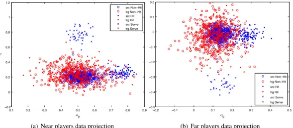
3.1.4 Feature Space Visualisations . . . 57

3.2 Chars74K Digit Dataset . . . 61

3.3 MNIST-USPS Database . . . 62

3.4 Caltech+Office Database . . . 64

3.5 COIL20 Dataset . . . 65

4 Posterior Adaptation via Feature Space Transformation

71

4.1 Introduction . . . 72

4.2 Related Work . . . 73

4.3 Feature Space Class-conditional Transformations . . . 75

4.3.1 Arnold

et al. ’s Method and Proposed Modifications (Reweight) . . . . 76

4.3.2 Translating and Scaling Features (TST) . . . 79

4.4 Experiments and Results . . . 81

4.4.1 Synthetic 3-Class Dataset Experiment . . . 81

4.4.2 Transfer from Tennis Single to Double Matches . . . 81

4.4.3 Badminton Dataset Experiment . . . 85

4.4.4 Transductive Transfer with Additional Target Adaptation Set . . . 86

4.5 Summary . . . 90

5 Transductive Transfer Machine

95

5.1 Related work . . . 97

5.2 Marginal and conditional distribution adaptation . . . 97

5.2.1 Shared space detection with MMD . . . 100

5.2.2 Sample-based adaptation with TransGrad . . . 102

5.2.3 Conditional distribution adaptation with TST . . . 104

5.2.4 Iterative refinement of the conditional distribution . . . 106

5.2.5 Stopping criterion . . . 106

5.2.7 The TTM algorithm and its computational complexity . . . 109

5.3 Experimental Evaluation . . . 110

5.3.1 Experiments and Results . . . 111

5.4 Summary . . . 120

6 Conclusions and Future work

123

6.1 Conclusion . . . 124

6.2 Future Work . . . 126

A Transductive Random Forest

129

A.1 Related Work . . . 130

A.2 Decision Trees . . . 131

A.2.1 Tree training (off-line) . . . 132

A.2.2 Tree testing (runtime) . . . 135

A.3 Random Forest . . . 135

A.3.1 The training objective function of Random Forest . . . 136

A.3.2 The randomness model . . . 136

A.3.3 The ensemble model: RF . . . 137

A.4 Semi-supervised Random Forest . . . 137

A.4.1 The Training objective function for Semi-supervised Random Forest . . 138

A.4.2 Label propagation for SSRF . . . 139

A.4.3 The ensemble model: SSRF . . . 140

A.5.1 The training objective function . . . 140

A.5.2 The randomness model . . . 142

A.6 Adaptive Transductive Random Forest . . . 143

A.7 Experiments and Results . . . 143

A.7.1 Two-Moons Synthetic Dataset Experiments . . . 144

A.7.2 Experiments on the Chars74K Dataset . . . 153

A.8 Summary . . . 162

B Additional Results

165

B.1 Iterative Algorithms for TST Domain Adaptation . . . 165

1.1 Traditional Machine Learning vs. Transfer Learning . . . .

4

1.2 TTL Applications . . . .

7

2.1 HOG3D Diagram . . . 16

2.2 SURF BoW Diagram . . . 18

2.3 CNN structure . . . 19

2.4 PCA . . . 22

2.5 Transfer Learning Diagram . . . 33

3.1 A detailed diagram of the tennis video analysis system . . . 48

3.2 A simplified diagram of the tennis video analysis system (taken from [85]). . . 49

3.3 An illustrative example of the composition of a tennis video. The length of

each shot is proportional to the width of the corresponding block in the figure

(taken from [85]). . . 49

3.4 Shot types: (a) crowd (b) close-up (c) play (d) commercial. . . 50

3.5 The GUI of the tennis video annotation system [85]. . . 51

3.6 Tennis Data: Player-Actions Samples . . . 53

3.7 Badminton Data: Player-Actions Samples . . . 54

3.8 Tennis and Badminton Annotation Tool . . . 56

3.9 Tennis Data HoG3D Correlation Matrix . . . 58

3.10 Tennis Data Projection in LDA Space . . . 59

3.11 Tennis Data: Source and Target Kernels . . . 60

3.12 Chars74k Database . . . 62

3.13 USPS Database . . . 63

3.14 MNIST . . . 64

3.15 Caltech+Office Database . . . 66

3.16 COIL20 Dataset-1 . . . 67

3.17 COIL20 Dataset2 . . . 68

4.1 Linear source clusters scaling: the binary classification task where the squares

and crosses are representing the samples of each class; the source clusters in

the left panel are scaled to better demonstrate the target distribution of the right

panel. . . 79

4.2 Linear source clusters translation and scaling: he binary classification task

where the squares and crosses are representing the samples of each class; the

source clusters in the left panel are scaled and translated to better demonstrate

the target distribution of the right panel. . . 80

4.4 Distance Metric Evaluations for KDA Kernels . . . 82

4.6 Tennis Data: Badminton vs Different Tennis Singles Datasets . . . 85

4.7 Serve detection failure in transfer from Badminton to Tennis, due to their

dif-ferent visual appearance. . . 88

4.3 Synthetic Data: Graphical Results . . . 92

4.5 Tennis Data: Numerical Results vs Transfer Rate Variations . . . 93

4.8 Tennis Data: Single vs Double New Results . . . 93

5.1 Public Data: 2D Projected Graphs of TTM Performance . . . 98

5.2 TTM Diagram . . . 110

5.3 Bar chart demonstrating the same results of Table5.4. . . 114

5.4 Bar chart demonstrating the same results of Table5.6 . . . 118

5.5

D

clusters

vs. averaged accuracy enhancement over the PCA baseline graph for

Table5.3 transfer tasks. . . 119

5.6

D

global

vs. averaged accuracy enhancement over the PCA baseline graph for

Table5.3 transfer tasks. . . 120

5.7 The effect of different

00

values and number of GMM clusters in the

Trans-Grad step of our framework on the final performance of the pipeline for three

cross- domain experiments. Constant lines show the baseline accuracy for each

experiment. . . 121

6.1 Future Work Diagram1 . . . 128

A.1 Decision Tree Flowchart . . . 132

A.2 Tree Testing (runtime Phase) . . . 133

A.3 Twisted Moons: Graphical Results with DT, RF and SSRF . . . 145

A.4 Translated and Scaled Moons: Data Representations . . . 148

A.5 Translated and Scaled Data: Transfer Parameter Estimation Graphs . . . 149

A.7 Char74 Data: Noise Insertion Images . . . 154

A.8 Char74: Transductive-SSRF Results . . . 155

A.9 Char74: Transductive-SSRF Results (Futher Experiments) . . . 156

A.10 Char74: Fine Evaluations of the Transductive-Tree Failure Case (Graphical

Representation) . . . 158

A.11 Char74: Transformation Estimation with Transductive-SSRF (Failure

Case-Study) . . . 159

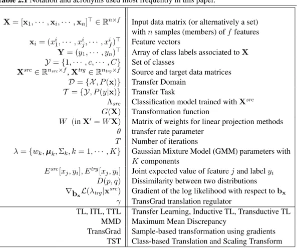
2.1 Notation and acronyms used most frequently in this paper. . . 15

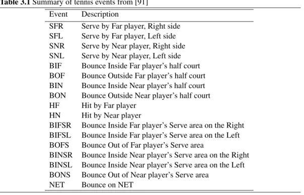
3.1 Summary of tennis events from [91] . . . 52

3.2 Tennis Data: Clusters Data-Distributions . . . 53

3.3 Comparison between Tennis and Badminton. Note that, in the table, match

intensity refers to the actual time the ball/shuttle was in flight, divided by the

length of the match. . . 55

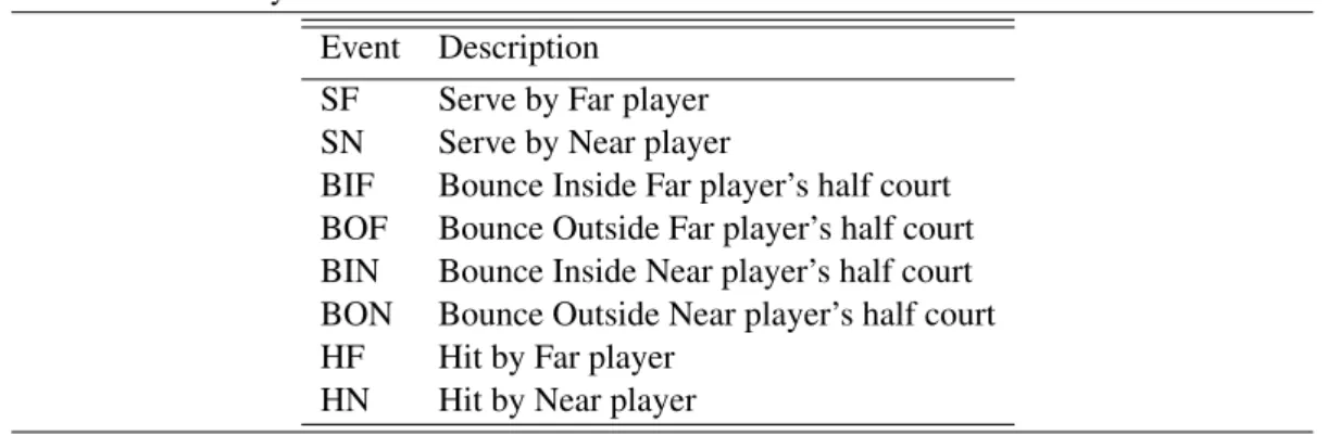
3.4 Summary of Badminton events . . . 57

3.5 USPS data distribution [31]. . . 63

4.1 Tennis Data: semi-Supervised Domain Adaptation Exp.1 . . . 87

4.2 Tennis Data: semi-Supervised Domain Adaptation Exp.2 . . . 89

5.1 Classifier selection and model adaptation . . . 108

5.2 Classifiers evaluations on individual domains: 5-fold cross validation accuracy

of a nearest neighbour classifier. All the datasets are

l2-normalized. . . 111

5.3 Cross-domain dissimilarities between domains (src

!

trg

), with datasets

ab-breviated as M: MNIST, U: USPS, C: Caltech, A: Amazon, W: Webcam, and

D: DSLR. . . 112

5.4 Recognition accuracies with datasets abbreviated as M: MNIST, U: USPS, C:

Caltech, A: Amazon, W: Webcam, and D: DSLR. Comparisons start the

base-line accuracy with NN and PCA followed by the results of the discussed TTL

algorithms. The last two columns show the effect of the classifier selection and

model adaptation techniques (5.2.6) on JDA and TTM algorithms. . . 113

5.5 Recognition accuracies with NN classifiers on target domains using differnet

shared subspace projection methods. . . 116

5.6 Results on Caltech+office dataset using DeCAF features. . . 117

A.1 Twisted Moons: Numerical Results . . . 146

A.2 Moons: DT, RF and SSRF Numerical Performance Comparisons . . . 153

A.3 Char74: DT vs Transductive-SSRF Numerical Results . . . 160

A.4 Char74: Effect of PCA Dimensionality Reduction before Applying the TL

Al-gorithm . . . 161

A.5 Char74: ERF, TRf and ATRF Performance Evaluations . . . 161

A.6 Public Data: JDA, Transductive-SSRF and NN-TST Performance Evaluations . 162

A.7 Public Data: Transductive-RF vs Transdutive-SSRF and NN . . . 162

Introduction

As human beings, our learning capacity develops progressively in time as we grow. At the age

of six, we recognise around 104 object categories and we keep learning more throughout our

life [13]. Moreover we tend to semantically organise all our knowledge into meaningful

tax-onomies: concepts and categories are grouped on the basis of the common properties acquired

through our five senses [3, 32, 55]. This intrinsically means that any new concept is not learned

in isolation, but considering connections to what is already known, which makes analogical

reasoning (the skill of building analogies) one of the cores of human intelligence [71]. This

results in practical advantages: it might be easier to learn French if one already knows Italian

and English and it might be easier to learn playing badminton if one already knows tennis.

In the context of computer vision, an image in the most basic representation is defined through a

matrix of its pixels intensity values and the semantic organisation of an image database is know

as classification where an ideal image classifier should be able to exploit complex high

dimen-sional feature representations even when only a few labelled training samples are available. In

most classification scenarios, it is expensive to acquire vast amounts of labelled training

sam-ples in order to provide classifiers with a good coverage of the feature space. One possible way

of dealing with this problem is to synthesise images of training objects using computer graphics

techniques (e.g. [147]), but their appearance may not be realistic and it is not possible to model

all possible backgrounds. Practitioners often resort to crowd sourcing [19], but the annotations

obtained are either costly or unreliable. Ideally, an image classifier should be initially capable

of detecting similarities between data distributions and subsequently facilitates the exploitation

of the required knowledge from all the previously trained reliable models, just as human can

exploit previous experience when learning some similar concepts.

For example, when a child learns to recognise a new letter of the alphabet he will use

exam-ples provided by people with different hand-writing styles, using pens of different colors and

thicknesses. Without any prior knowledge a child would need to consider a large set of

fea-tures as potentially relevant for learning the new concept, so we would expect the child to need

a large number of examples. But if the child has previously learnt to recognise other letters,

he can probably discern the relevant attributes (e.g. number of lines, line curvatures) from the

irrelevant ones (e.g. the colour of the lines) and learn the new concept with fewer examples.

This observation suggests that a sample efficient image classification algorithm might need to

exploit knowledge gained from related tasks.

In the absence of such prior knowledge, a typical image classification task would require the

exploration of a large and complex feature space. In such high dimensional feature spaces

some features will be discriminative while most probably a large number of them are irrelevant.

Additionally, out of this set of discriminative features some might help in detecting the relations

in between similar tasks and hence be beneficial for a new related concept classification. While

we do not know a-priori what features are irrelevant, related tasks might share these features

and we can use training data from these tasks to discover them.

An initial step to this task and feature relevancy discovery is to first be able to tell which tasks

can be classified as similar. While many recent works [53, 52, 138] studied this as zero-shot

learning, in this thesis we assumed that our system is already aware of the task similarities

between the two training (source) data an a given new unlabelled test (target) data.

The goal of this thesis is to develop efficient transfer learning algorithms for image

classifica-tion that can exploit rich feature representaclassifica-tions.

1.1 Problem: Transfer Learning for Computer Vision

Recently, there has been a significant growth in multimedia data production. This data exists

in various different forms such as broadcast content (including television, DVDs, BluRays and

Internet) and personal content (e.g. uploads from hand-held devices); it can also be recorded

interviews or meetings, or footage from surveillance cameras. Most of this data is intended

for general viewing and hence basic labelling (Date, Time and Title etc.) is attached to it

which is often inaccurate. However in many cases it would be useful to add additional labels

to retrieve information in a more flexible and systematic fashion (e.g. a Tennis sports video can

potentially be labelled with match-events description). Such meta-data will assist in finding

material within the multimedia footage via browsing, querying or searching.

For easy retrieval of information from a very large quantity of archived images of videos, it

would be very useful to have them annotated

automatically i.e. to create a system that could

understand the visual content (manual annotation being too unwieldy). The annotation task can

become even more challenging when the new test data does not follow the same distribution

as of the initial training data. Unlike traditional machine learning methods, transfer learning

methods do not assume that training and test data are drawn from the same distribution [123],

hence fitting well to this annotation problem.

Traditionally, machine learning algorithms were training models separately even for similar

training domains. Transfer Learning algorithms try to alleviate the training by benefiting from

the relations between similar domains. Figure 1.1 illustrates the difference between the

learn-ing process of traditional machine learnlearn-ing and transfer learnlearn-ing. As we can see, traditional

machine learning techniques try to learn each task from scratch, while transfer learning

tech-niques try to transfer the knowledge from some previous task(s) to a target task when the latter

has fewer high-quality or labelled training data [123].

⇥⇤⌅⇧⌃⇧⌥ ⇤ ⌦↵ ⌦ ✏⌦

⇥⇤⌅⇧⌃⇧⌥ ⇤ ⌦↵ ⌦ ✏⌦

⇥⇤⌅⇧⌃⇧⌥ ⌅⌦↵⇥

⌦

⇥⇤⌅⇧⌃⇧⌥ ⌅⌦↵⇥

⌦

⌅⇤✏⌃⇣⌃⌦⇧⇤⌘ ✓

⌅⇤✏⌃⇣⌃⌦⇧⇤⌘ ✓

⇥⇤⌅⇧⌃⇧⌥ ⌅⌦↵⇥

⌦

⇥⇤⌅⇧⌃⇧⌥ ⌅⌦↵⇥

⌦

⌅⇤⇧ ⇥⌅ ⇥⇤⌅⇧⌃⇧⌥

⌅⇤⇧ ⇥⌅ ⇥⇤⌅⇧⌃⇧⌥

⇣⌅⇤⌃⇧⌃⇧⌥ ⌃⇣⇥◆

⇣⌅⇤⌃⇧⌃⇧⌥ ⌃⇣⇥◆

⇣⇤⇥ ⇧ ⌘⌦✓◆ ⌃⇣

⇣⇤⇥ ⇧ ⌘⌦✓◆ ⌃⇣

⇣⌅⇤⌃⇧⌃⇧⌥ ⌃⇣⇥◆

⇣⌅⇤⌃⇧⌃⇧⌥ ⌃⇣⇥◆

⇣⇤⇥ ⇧ ⌘⌦✓◆ ⌃⇣

⇣⇤⇥ ⇧ ⌘⌦✓◆ ⌃⇣

⇥⇤⌅⇧⌃⌥ ⌃

⇥⇤⌅⇧⌃⌥ ⌃

The field of transfer learning includes a range of problems in which there is a change of domain

or task between source and target sets. Transfer learning techniques are becoming more popular

in Computer Vision, particularly after Torralba and Efros [151] discovered significant biases in

object classification datasets.

Based on Pan and Yang’s survey [123], Transfer Learning (TL) can be categorised into three

types of approaches; Inductive Transfer Learning (ITL) where some labelled data in the

tar-get domain are required to induce an objective predictive model for use in the tartar-get domain,

Transductive Transfer Learning (TTL) where no labelled data in the target domain are available

at the training time, and finally Unsupervised Transfer Learning (UTL) where no labelled data

is available in source or target domains. While much of the work focuses on

inductive

transfer

learning problems, which assume that labelled samples are available both in the training/source

and test/target domains, in this thesis we focus on the case in which only unlabelled samples are

available in the test/target domain. This is a

transductive

transfer learning (TTL) problem, i.e.,

the joint probability distribution of samples and classes in the source domain,

P

(X

src

,

Y

src

), is

assumed to be different, but related to that of a target domain joint distribution,

P

(X

trg

,

Y

trg

),

but labels

Y

trg

are not available in the target set. We follow a similar notation to that of [123]

(see Table 2.1).

Transductive transfer learning methods can potentially improve a very wide range of

classifica-tion tasks, as it is often the case that a domain change happens between training and applicaclassifica-tion

of algorithms, and it is also very common that unlabelled samples are available in the target

domain.

The main focus of this thesis is then in looking for a common latent representation and data

transformation techniques which reduce the dissimilarities of the data configuration in the

source (training) and the target (test) domains after transformation.

Recent advances in computer vision and machine learning as well as the exponential growth

in the processing capacity and memory of computer technology have created the conditions

where it becomes timely to investigate the possibility of designing such systems.

One of the applications is in sports footage which provides a useful test-ground given its fixed,

rule-governed content. To date, there have been several annotation systems developed for

different sports such as football [164], Formula 1 [128], snooker [40] and Tennis [39]. As

part of the work on video data, we focus specifically on court-based games, such as Tennis and

Badminton. We build upon the outcome of a previous project ACASVA (Adaptive Cognition

for Automated Sports Video Annotation) to perform automatic adaptation of the trained system

so that it can be applied to a different game. For instance if the main system has been trained to

interpret a Tennis single match, we aim to transfer this learning to either Tennis doubles game

or even a different domain such as Badminton.

Another example is in image classification where the training set may come from high quality

images (e.g. from DSLR cameras) and the target test set may come from mobile devices.

Fig-ure 1.2 demonstrates instances from three different classes obtained from these two relevant

domains. As one can note the image quality, illumination level and background varies from

one domain to other. TTL methods can potentially generalise classification methods for a wide

range of domains and make them scalable for big data problems.

In this thesis, we employ transformative approaches for solving the transductive transfer

learn-ing problem in which feature transformations are used to adapt the source domain feature

dis-tributions to the target domain. In essence, linear and non-linear joint adaptation of marginal

and conditional distributions of the source and target data are introduced.

1.2 Contributions

The main contribution of this thesis can be listed as follows:

•

Unsupervised adaptation of the conditional distributions:

We propose unsupervised

class-specific transformations for domain adaptation. The technique is based on

estimat-ing linear transformations to adapt the source domain features in order to maximise the

similarity between posterior probability distribution functions (PDF) for each class in

Figure 1.2: Sample images with varying image acquisition quality. Right: sample images

captured by a Webcam camera, Left: images obtained from Amazon webpage .

the source domain and the expected posterior PDF for each class in the target domain

(Chapter 4).

•

Joint adaptation of the marginal and conditional distributions:

We propose Transductive Transfer Machine (TTM) algorithms which combine methods

that adapt the marginal and the conditional distribution of the samples, so that source and

target datasets become more similar, facilitating classification (Chapter 5).

•

Two unsupervised dissimilarity measures for automating the parameter setting of

the proposed data processing pipeline for a new transfer task:

Two dissimilarity measures are devised which enable the proposed pipeline to

automat-ically readjust its parameters for a new transductive transfer task where the source and

target distributions are from different environments (Chapter 5).

•

A classifier selection and model parameter adaptation algorithm:

We proposed Adaptive Transductive Transfer Machine (ATTM) which uses the afore

mentioned dissimilarity measures to select the right classifier and to optimise its

param-eters for a new target domain. We show that our method obtains state-of-the-art results

in cross-domain vision datasets using na¨ıve features, with a significant gain in

computa-tional efficiency in comparison to related methods (Chapter 5).

•

Assessment of semi-supervised random forest for transductive transfer learning:

We have also constructed a transductive transfer version of random forest and study its

performance on unsupervised/ semi-supervised domain adaptation problems (Appendix

A).

1.3 Outline

The structure of the thesis is as follows: Chapter 2 provides the necessary background on

fea-ture extraction methods and classification algorithms. Chapter 3 describes the databases with

their common protocols used in our experiments. In Chapter 4 two transfer learning

meth-ods are proposed and some modifications to the existing methmeth-ods are suggested (published in

[47, 49]). A novel transductive transfer learning pipeline is introduced in Chapter 5, published

in [48, 46]. Finally, in Chapter 6 we draw conclusions and discuss future lines of research. In

addition, in Appendix A we study the semi-supervised random forest and propose a

transduc-tive transfer random forest approach.

1.4 List of Publications

Parts of this thesis appeared in conference proceedings. The list of publications is as follows:

• N. FarajiDavar and T. deCampos and J. Kittler and F.Yang Transductive Transfer

Learn-ing for Action Recognition in Tennis Games (Poster) In 3rd International Workshop on

Video Event Categorization, Tagging and Retrieval for Real-World Applications

(VEC-TaR), in conjunction with 13th International Conference on Computer Vision(ICCV),

Barcelona, Spain 2011 [47]

• N. FarajiDavar and T. deCampos and D. Windridge and J. Kittler and W. Christmas

Do-main Adaptation in the Context of Sport Video Action Recognition (Poster) In DoDo-main

Adaptation Workshop, in conjunction with NIPS, Sierra Nevada, Spain 2011 [49]

• N. Farajidavar, T. de Campos, D. Windridge, J. Kittler, W. Christmas. Domain

Adapta-tion in the Context of Sport Video AcAdapta-tion RecogniAdapta-tion (Poster), 4th UK Computer Vision

Student Workshop (BMVW), in conjunction with the British Machine Vision Conference

(BMVC), Guildford, September 2012 [50]

• N. Farajidavar, T. de Campos, J. Kittler. Transductive Transfer Machine, In Proceedings

of Asian Conference on Computer Vision (ACCV), Singapore, 01 November 2014 [48]

• N. Farajidavar, T. de Campos, J. Kittler. Adaptive Transfer Machine, In Proceedings of

Background

In this chapter, we review the theoretical concepts, technical ideas and background knowledge

on feature extraction, classification and transfer learning. We also give a brief review of some

of the apparatus used in the rest of this thesis.

The goal of classification is to take an input vector

x

2

X

and to assign to it a discrete class

label

y

2

Y

, where the number of classes is

C

=

|Y|

. In the most common scenario, the

classes are taken to be exclusive, so that each input is assigned to one and only one class. The

input space

X

is thereby divided into decision regions whose boundaries are called decision

boundaries or decision surfaces.

The first step is to describe the data in an appropriate manner. In the case of video, a space-time

descriptor is used for that, generating a vectorial representation

x. This may be followed by a

feature extraction and feature selection method to reduce the dimensionality and improve the

discrimination power.

Data sets and parameters can easily get outdated or the training data may not always facilitate

a direct generalisation to the test data. Also, one may need to use knowledge from one domain

for application in another domain (e.g. detection of Spam learnt in English applied to French

emails). Such issues are addressed by transfer learning techniques which are motivated by the

fact that people can intelligently apply knowledge learned previously to solve new problems

faster or with better solutions in different (but related) domains.

The focus of this work is on transfer learning, which is reviewed in Chapter 4 . But before

that, in order to provide background for our experiments, we briefly review the methods used

for feature extraction and classification in Sections 2.2 and 2.4, respectively. In Section 2.5

we define the Transfer Learning in mathematical terms and briefly review the litreture of its

taxnomy and variations.

2.1 Notation

This section is a reference for the remaining of this thesis, where we introduce some

nota-tion and defininota-tions. In image and acnota-tion classificanota-tion, as in most classificanota-tion problems,

systems are trained with samples from one set up and often expected to be applied to

an-other set up. Given a sample

x

and a class label

y, the standard statistical classification

task is to assign a probability,

p(y

|

x), to the event of

x

belonging to class

y. In the binary

classification case the labels are

y

2

{

0,

1

}

. Typically, each example

x

i

is represented as

a vector of features

(x

1

i

,

· · ·

, x

f

i

,

· · ·

, x

F

i

)

where

F

is the number of features or

dimen-sions of the feature space (e.g.

X

=

R

F

). The data consists of two disjoint subsets; the

training set

(Xtrain, Ytrain) =

{

(x1, y1),

· · ·

,

(xntrain

, yntrain

)

}

, (e.g. sample feature vectors

obtained from a set of people in a set of environments, illumination conditions, camera

config-urations/types and with certain types of background) available to the model for its training and

the test set

Xtest

=

{

x1, ...,

xntest}

, upon which we want to use our trained classifier to make

predictions. A pattern recognition system is expected to perform well if the test samples

X

test

are obtained in the same conditions as

X

train

,

e.g. if they are new videos of the same people

performing the same actions in the same environments as before.

However, in most application scenarios there is a change of scene, video/image quality,

per-forming actors

etc., so although the domain representation and the label set are the same,

i.e.

X

train

=

X

test

and

Y

train

=

Y

test

, the data distributions are different,

i.e.

p(X

train

)

6

=

p(X

test

).

The two most important definitions in the transfer learning paradigm are those of

Domain

and

Task. A domain is composed of two components: a feature space

X

and a marginal probability

distribution

P

(x), where

x

=

{

x

1

,

· · ·

, x

F

}

2

X. Given a specific domain,

D

=

{X

, P

(x)

}

,

a task

T

consists of two components: a label space

Y

and an objective predictive function

P

(y

|

x). Generally in transfer learning the knowledge obtained from one or more source

do-mains can be used for classification in a new target domain. In the simplest mode we assume

that there exist two domains and two tasks, consisting of source domain,

D

src

and target

do-main,

D

trg

and similarly source and target tasks,

T

src

and

T

trg

respectively. In such

circum-stances transfer learning is proposed as a solution.

For ease of notation,

x

i

j

is the feature

j

of sample

x

i

and

E

src

[x

j

, y]

is used to represent

E

X

src

[x

j

, y]

which is the expected value of the feature

x

j

with label equal to

y,

8

x

2

X

src

and

n

src

train

is the number of labelled training data in the source domain.

The usual traditional machine learning approach is to assume

D

train

⇡

D

test

, and treat this as a

classical generalisation problem in machine learning by means of classifier regularisation [14].

In our problem

D

train

6

=

D

test

. It characterises a special case of

transductive transfer

learn-ing

which has not been covered by Pan and Yang [123] transfer learning survey where both

domain and task are differing from source to target and we do not have access to any labels in

the new target domain: we then aim to improve the learning of the target predictive function

P

(Y

trg

|

X

trg

)

in

D

trg

using the knowledge in

D

src

and

T

src

, where

D

src

6

=

D

trg

.

The solution to such a task will be either transforming the domains in a way that both domains

become more similar or introducing some adaptive classifier which can be generative enough

to fit well the new target domain. For that, we evaluate two methods that transform the features

of

X

src

so that they become more similar to

X

trg

and the classifier is re-trained using the

transformed samples.

The most frequently used notation of this work is summarised in Table 2.1.

2.2 Feature Extraction Methods for Image and Video in Computer

Vision

As in any machine learning architecture, the first step in learning is to efficiently represent

interesting parts of an image (or video) as a compact feature vector which ins known as

feature

extraction

[155]. The goal is to come up with a vectorial representation that is discriminative

enough for a later classification purpose.

Table 2.1

Notation and acronyms used most frequently in this paper.

X

= [x1,

· · ·

,

xi,

· · ·

,

xn]

>

2

R

n

⇥

f

Input data matrix (or alternatively a set)

with

n

samples (members) of

f

features

x

i

= (x

i

1

,

· · ·

, x

j

i

,

· · ·

, x

i

f

)

>

Feature vectors

Y

= (y

1

,

· · ·

, y

n

)

>

Array of class labels associated to

X

Y

=

{

1,

· · ·

, c,

· · ·

, C

}

Set of classes

X

src

2

R

nsrc

⇥

f

,

X

trg

2

R

ntrg

⇥

f

Source and target data matrices

D

=

{X

, P

(x)

}

Transfer Domain

T

=

{Y

, P

(y

|

x)

}

Transfer Task

⇤

src

Classification model trained with

X

src

G(X)

Transformation function

W

(in

X

0

=

W

X)

Matrix of weights for linear projection methods

✓

transfer rate parameter

T

Number of iterations

=

{

w

k

,

µ

k

,

⌃

k

, k

= 1,

· · ·

, K

}

Gaussian Mixture Model (GMM) parameters with

K

components

E

src

[x

j

, y

i

], E

trg

[x

j

, y

i

]

Joint expected value of feature

j

and label

y

i

D(p, q)

Dissimilarity between two distributions

r

bx

L

(

trg

|

x

src

)

Gradient of the log likelihood with respect to

b

x

TransGrad translation regulator

TL, ITL, TTL

Transfer Learning, Inductive TL, Transductive TL

MMD

Maximum Mean Discrepancy

TransGrad

Sample-based transformation using gradients

TST

Class-based Translation and Scaling Transform

In this section we will provide a brief background on the feature extraction methods which has

been utilised in this thesis. In summary, for Player Action (video) datasets we used HoG3D

which is a three dimensional generalisation of SIFT or local histograms of oriented gradients

(HOG). As for the image datasets, we utilised two types of feature extractions: Bag-of-SURF

and Convolutional Neural Network features.

2.2.1 Histograms of Oriented Gradients in 3D Space-time Blocks (HOG3D)

In order to extract a feature vector

x

to describe a video segment a range of methods are

available in literature. We used HOG3D [89] descriptors for our task because it was among the

top performing method according to Wang

et al.’s survey [153].

HOG3D is a three dimensional generalisation of SIFT [108] or local histograms of oriented

gradients (HOG) [35]. It uses polyhedral structures for the quantisation of the 3-D

spatio-temporal edge orientations to avoid the singularities in the use of polar coordinate systems (as

advocated in [145]). Another advantage of HOG3D [89] is its computational efficiency due to

the use of three-dimensional integral images.

Given a spatio-temporal block, HOG3D splits it into

M

⇥

M

⇥

N

sub-regions (M

for spatial

and

N

for temporal splits). Within each region, this method counts how many 3D gradients

are roughly aligned with each of the directions of a polyhedral structure. Figure 2.1 illustrates

the spatio-temporal divisions of the HOG3D descriptors. In [89] the authors claim that the best

performance in the validation set of the KTH [95] dataset was obtained with an icosahedron

(i.e., 20 orientations),

M

= 4

and

N

= 3, giving a total of 960 dimensions. The temporal

and spatial support of such descriptors were also optimised in [89], using the validation set of

KTH.

Figure 2.1: Kl¨aser

et al.’s HOG3D Diagram, ©authors of [89].

In this work HOG3D is used as a descriptor for STS-based action matching (STS:

Spatio-Temporal Shapes). But, in contrast to STS introduced in [65], HOG3D extracts information

from within the foreground gray-scale patches, rather than only describing the outline of binary

blobs. Since it describes 3D bounding boxes, it is also less affected by fragmentation problems

in segmentation.

In the STS-based experiments of de Campos

et al

. [37], a single HOG3D descriptor is extracted

for each detected actor at the time instance in which the action is classified. The extracted 960D

vector is then passed directly to a classifier instead of using bags-of-visual-words. For problems

in which the aim is to classify the activity in a video sequence rather than an instantaneous

action, they use HOG3D at a number of temporal windows within a video sequence. The

classification results are then combined using a voting scheme.

2.2.2 Bag of Visual Words

The bag-of-visual-words uses a simple assumption from natural language processing and

in-formation retrieval, and has been widely applied in computer vision. In general, there are three

main steps for the model: (i) initially the local SURF [11] descriptors are obtained to describe

the interest points; (ii) these descriptors are then quantised by K- means clustering to form

a codebook; (iii) images are eventually represented as the K-dimensional histograms of the

visual words [76]. The procedure includes two parts: learning and recognition.

For each image, interest points are sampled and the local descriptors are extracted. While any

existing interest point detectors and descriptors can be used for this step, a common approach

proposed in [11] is to use the SURF descriptor.

Inspired by SIFT [109], the SURF descriptors are claimed to be faster and more robust against

different image transformations. It is based on an integer approximation of the determinant of

the Hessian blob detector which can be computed extremely quickly with an integral image.

Secondly, these descriptors are quantised by K-means clustering to form a codebook. Finally,

images can be represented as the K-dimensional histograms of the visual words.

2.2.3 Deep Convolutional Activation Feature (DeCAF)

In order to better evaluate our proposed approaches, we have also utilised the state-of-the-art

CCN [41, 93, 27] features for representing our image data.

Figure 2.2: A typical processing pipeline for a bag-of-word category recognition system

re-produced from [125]. Features are first extracted at key-points and then quantised to get a

distribution (histogram) over the learned

visual words

(feature cluster centers). The feature

distribution histogram is used to learn a decision surface using a classification algorithm such

as support vector machines [150].

Natural images have the property of being stationary, meaning that the statistics of one part of

the image are the same as any other part. This suggests that the features that we learn at one

part of the image can also be applied to other parts of the image, and we can use the same type

of feature at all locations.

More precisely, having learned features over small (

i.e

.

8

⇥

8) patches sampled randomly from

larger image, we can apply this learned

8

⇥

8

feature detector anywhere in the image.

Specif-ically, we can take the learned

8

⇥

8

features and convolve them with the larger image, thus

obtaining a different feature activation value at each location in the image.

A typical Convolutional Neural Network (CNN) architecture is shown in Figure 2.3. In a

fully-connected network, the output of each hidden activation unit

h

i

is computed by multiplying the

entire input

x

by weights

W

in that layer. However, in a CNN, each hidden activation output

is computed by multiplying a small local input (i.e.

[x1, x2, x3]) against the weights

W

. The

weights

W

are then shared across the entire input space. After computing the output of the

hidden units, a max-pooling layer helps to remove variability in location, scale and orientation

of image content. Specifically, each max-pooling unit receives activations from a bank of

convolutional bands, and outputs the maximum of the activations from these bands.

Figure 2.3: Convolutional Neural network structure (©Torch7 documentation [27]): A CNN

is a trainable architecture composed of multiple convolution and pooling stages.

For example, if the input is a colour image, each feature map would be a 2D array containing a

colour channel of the input image (i.e. for a video or volumetric image, it would be a 3D array).

At the output, each feature map represents a particular feature extracted at all locations on the

input. Each layer in the network is composed of three steps: a filter bank step, a non-linearity

step, and a feature pooling step. A typical CNN is composed of one, two or more such 3-step

layers, followed by a classification module. The steps are further described for the case of

image recognition:

•

Filter bank step

: the input is a 2D array feature map denoted as

x

i

. The output is also

a 2D array feature map,y. A trainable filter (kernel)

kij

in the filter bank connects input

feature map

xi

to output feature map

yj. The module computes

yj

=

bj

+

Wkij

⇤

xi

where * is the 2D discrete convolution operator and

b

j

is a trainable bias parameter.

Each filter detects a particular feature at every location on the input. Hence spatially

translating the input of a feature detection layer will translate the output but leave it

otherwise unchanged.

•

Non-linearity step: In traditional CNN this simply consists in a pointwise hyperbolic

tangent (tanh()) sigmoid function applied to each site (x

ijk

). However, recent

imple-mentations have used more sophisticated non-linearities. A useful one for natural image

recognition is the rectified sigmoid Rabs:

|

gi.tanh()

|

where

gi

is a trainable gain

pa-rameter. The rectified sigmoid is sometimes followed by a subtractive and divisive local

normalisation, which enforces local competition between adjacent features in a feature

map, and between features at the same spatial location.

•

Feature pooling step: This step treats each feature map separately. In its simplest

in-stance, it computes the average values over a neighborhood in each feature map. Recent

work [154, 29] has shown that more selective poolings, based on the LP-norm, tend to

work best with a

2

⇥

2

subsampling or alternatively by max pooling instead of

averag-ing. The later approach forces the network to capture the most useful local features that

are produced by the convolutional layers. The neighborhoods are stepped by a stride

larger than one (but smaller than or equal the pooling neighborhood). This results in a

reduced-resolution output feature map which is robust to small variations in the location

of features in the previous layer.

The output of this 3-step image alterations is known as the feature map of the

l

th

layer in the

network. According to the granularity level of interest in terms of the substructures within an

image, the output of different stages of the network can be selected as the image descriptors.

In our experiments we confined ourself to using the output of the

6

th

network layer.

2.3 Feature Selection

Feature selection methods evaluate an optimality criterion for combinations of

f

variables and

select that combination for which this criterion is maximised. The goal is to disregard those

variables that do not contribute to class separability to speed up the final training process. In

our experiments, we have used a range of dimensionality reduction algorithms to enhance our

final training. In this section, we will briefly describe these techniques.

2.3.1 Principal Component Analysis

Principal component analysis (PCA) tries to derive new variables that is a linear combination of

the original ones and are uncorrelated. The most common definition of PCA, by Hotelling [74],

is that, for a given set of data vectors

x

i

, i

2

1

, ..., n

the

k

principal axes are those orthonormal

axes onto which the variance retained under projection is maximal. Geometrically, PCA can

be thought of as a rotation of the axes of the original coordinate system to this new set of

orthogonal axes that are ordered in terms of the amount of variation of the original data they

account for [155].

In order to capture as much of the variability as possible, let us choose the first principal

com-ponent, denoted by

U

1

[60]. Suppose that all centred observations are stacked into the columns

of an

f

⇥

n

matrix

X

>

, where each column corresponds to an f-dimensional observation and

there are

n

observations. Under this notation principal components can be described as linear

projections of

X

defined by weight vector

w

i

.

We choose

W

to maximise

W

>

⌃

W

while constraining

W

to have unit length where

⌃

is the

f

⇥

f

sample covariance matrix of

X

observations.

max

W

>

⌃

W

subject to

W

>

W

= 1

(2.1)

The solution can be expressed as the singular value decomposition (SVD) of the covariance

matrix,

⌃

:

⌃

=

U SV

>

(2.2)

where matrix

S

contains the eigenvalues of the covariance matrix of the observations on its

orthogonal and the columns of

U

in the SVD contain the eigenvectors of

⌃

. The training data

can be reconstructed as:

ˆ

X

=

U U

>

X

(2.3)

space where the data variance is maximised. A distribution of points drawn from a bivariate

Gaussian and centered on the origin of x-axis and y-axis is illustrated in Figure 2.4.

Figure 2.4: PCA projection defines a rotation such that the new axes (x’ and y’ corresponding

to

U1

and

U2

eigenvectors respectively) are aligned along the directions of maximal variance

(the principal components) with zero covariance. This is equivalent to minimizing the square

of the perpendicular distances between the points and the principal components.

Note that PCA does not take class labels into account. In the next section we will introduce the

Linear Discriminant Analysis (LDA) method which does it.

2.3.2 Linear Discriminant Analysis

Linear discriminant analysis (LDA), also known as Fisher’s linear discriminant, tries to find a

linear combination of features which separates two or more classes of objects or events.

From geometrical point of view the Fisher strategy is a projection of a high dimensional data

X

into a low dimensional space

R

C

1

. In the case of

C

-class problems the criterion is:

J

F

(

W

) =

W

>

§

B

W

W

>

S

w

W

(2.4)

where

S

B

is the between classes scatter (covariance) matrix and

S

w

is the within class

covari-ance matrix which are given by:

S

B

=

C

X

c

=1

n

i

n

(

µ

i

µ

)(

µ

i

µ

)

>

,

(2.5)

S

w

=

C

X

i

=1

n

i

n

⌃

i

(2.6)

where

c

= 1

,

· · ·

, C

and,

µ

i

and

⌃

i

are the sample means and covariance matrices of each

class and

µ

is the mean of all samples ignoring the class labels. The transformation matrix

W

can be found by solving the eigenvalues problem:

S

w

1

S

B

W

=

⇤

W

(2.7)

This

W

is a matrix of eigenvectors of

S

w

1

S

B

and

⇤

is a diagonal matrix of eigenvalues. This

means that when

W

i

is an eigenvector of

S

w

1

S

B

, the separability will be equal to the

corre-sponding eigenvalue. Since the rank of

S

B

is at most

C

1, then the eigenvectors associated

with non-zero eigenvalues identify the vector subspace containing the data.

In summery, the LDA dimensionality reduction can be achieved by:

• Compute the

f

-dimensional mean vectors for the different classes from the dataset.

• Compute the scatter matrices (between-class and within-class scatter matrix).

• Compute the eigenvectors and corresponding eigenvalues for the scatter matrices.

• Sort the eigenvectors by decreasing eigenvalues and choose k eigenvectors with the

rep-resents an eigenvector).

• Use this

f

⇥

k

eigenvector matrix to transform the samples onto the new subspace. This

can be summarised by the mathematical equation:

y

=

W

T

⇥

x

(where

x

is a

f

⇥

1

-dimensional vector representing one sample, and y is the transformed

f

0

⇥

1

-dimensional

sample in the new subspace).

2.4 Classification

The final step in supervised machine learning is training a classifier. Given a sample

x

and

a class label

y

, the standard statistical classification task is to assign a probability,

p

(

y

|

x)

or

alternatively a label,

y

ˆ

to the event of

x

where

y

denotes class membership. In the binary

classification case the labels are

Y

2

{

0

,

1

}

. Typically, each example

x

i

is represented as an

f

-dimensional vector of features. Below, we will brief the classification algorithms which we

utilised in this thesis.

2.4.1 Nearest Neighbor

Among the various methods of supervised statistical pattern recognition, the Nearest Neighbour

classifier achieves consistently high performance, without requiring any a priori assumptions

about the distributions from which the training examples are drawn. Given a training set of

both positive and negative samples, a new test sample,

x

, is classified by searching for the

nearest training point and assigning it the same label.

The k-NN classifier extends this idea by taking the

k

nearest points and assigning the label of

the majority. It is common to select

k

small and odd to break ties (typically 1, 3 or 5). Larger

k

values help to reduce the effect of outliers within the training data set, and the choice of

k

is

often performed through cross-validation.

As the size of training data set approaches infinity, the one nearest neighbour classifier

guar-antees an error rate of no worse than twice the Bayes error rate (the minimum achievable error

rate given the distribution of the data) [141].

2.4.2 Logistic Regression

Logistic regression is a probabilistic, linear classifier. It is parametrised by a weight vector

w

,

and a bias scaler

b

.

Given a data set

{

y

i

, x

i

1

, . . . , x

i

f

}

n

i

=1

of

n

statistical samples, a linear regression model assumes

that the relationship between the dependent variable

y

i

and the

f

-dimensional vector of

regres-sors

x

i

is linear. This relationship is modelled through a disturbance term or error variable

b

an

unobserved random variable that adds noise to the linear relationship between the dependent

variable and regressors. Thus the model takes the form

y

i

=

w

1

x

i

1

+

· · ·

+

w

f

x

i

f

+

b

= (xi)

>

w

+

b,

i

= 1

, . . . , n,

(2.8)

A large number of solutions have been developed for estimating the weight parameters out of

which the Ordinary Least Squares (OLS) is the simplest and thus the most common estimator. It

minimises the sum of squared residuals, and leads to a closed-form expression for the estimated

value of the unknown parameter

w

:

ˆ

w

= (X

>

X)

1

X

>

y

=

1

n

X

n

x

i

x

>

i

!

1

1

n

X

n

x

i

y

i

!

(2.9)

The estimator is unbiased and consistent if the errors have finite variance and are uncorrelated

with the regressors [98]. Alternatively maximum-likelihood estimation can be performed when

the distribution of the error terms is known to belong to a certain parametric family of

proba-bility distributions [124]. When this distribution is a normal distribution with zero mean and

variance , the resulting estimate is identical to the OLS estimate.

As for the logistic counterpart, the outputs of this linear layer are then fed to a softmax layer,

which produces a properly normalised probability distribution. Mathematically for a binary

classification task, it can be defined as:

P

(

y

i

= 1

|

x

i

,

w,

b

) =

1

1 +

e

(

x

>

i

w

+b)

(2.10)

The final prediction is typically done by choosing the label which maximises this distribution:

yi

= arg max

c

P

(

yi

=

c

|

xi,

w,

b

)

(2.11)

2.4.3 Support Vector Machines (SVM)

Support Vector Machines (SVM) algorithm invented by Vladimir N. Vapnik and Alexey Ya.

Chervonenkis are supervised learning models with associated learning algorithms that analyse

data and recognise patterns. Given a set of

n

training points of the form:

n

(

x

i

, y

i

)

|

x

i

2

R

f

, y

i

2

{

1

,

1

}

o

n

i=1

(2.12)

where the

yi

is either 1 or 1, indicating the class to which the point

xi

belongs. Each

xi

is an

f-dimensional real vector and the SVM classifier aims to find the maximum-margin hyperplane

which separates the points having

y

i

= 1

from those of class

y

i

=

1

. Any hyperplane can be

written as the set of points

x

satisfying

w

·

x

b

= 0

,

(2.13)

where ’

·

’ denotes the dot product and

w

the (not necessarily normalised) normal vector to the

hyperplane. The parameter

b

k

w

k

determines the offset of the hyperplane from the origin along

the normal vector

w.

If the training data are linearly separable, we can select two hyperplanes in a way that they

separate the data and there are no points between them, and then try to maximise their distance.

The region bounded by them is called

the margin. These hyperplanes can be described by the

equations

w

·

x

b

= 1

for

y

i

= 1

w

·

x

b

=

1

for

y

i

=

1

,

By using geometry, we find the distance between these two hyperplanes as

2

k

w

k

. In order to

maximise this distance we need to minimise

k

w

k

. As we also have to prevent data points from

falling into the margin, we add the following constraint: for each

i

either

w

·

x

i

b

1

for

y

i

= 1

w

·

x

i

b



1

for

y

i

=

1

,

This can be rewritten as:

y

i

(w

·

x

i

b

)

1

,

8

i,

1



i



n

(2.14)

We can put this together to get the optimisation problem:

min

w

,b

k

w

k

2

,

subject to

y

i

(w

·

x

i

b

)

1

.

(2.15)

This is a quadratic optimisation problem which assumes that the data is perfectly separable. To

deal with the non-separable case one can rewrite the optimisation problem as:

min

w

,b

k

w

k

2

+

C

n

X

i

=1

⇠

i

,

subject to

y

i

(w

·

x

i

b

)

1

⇠

i

.

(2.16)

where

⇠

i

0

and

C

is known as the margin parameter. The second term in eq. 2.16 can be

formulated as a training error function known as the Hinge Loss:

⇠

i

=

H

1

[

y

i

,

(w

·

x

i

b

)]

(2.17)

Quadratic Programming (QP) techniques.

While linear separation models are not always complex enough to describe the data, the

non-linear SVM maps data to a richer feature space including non-non-linear features, then constructs a

hyperplane in that space. Formally, we can pre-process the data by mapping it via a non-linear

function :

x

7!

(x)

(2.18)

and then learn the map from

(x)

to

y

subject to:

y

i

(w

·

(x

i

)

b)

1

⇠

i

,

8

i,

1



i



n

(2.19)

The dimensionality of

(x)

can be very large, making

w

hard to represent explicitly in

mem-ory, and hard for the QP to solve. The representer theorem [87] shows that for SVM as a special

case:

w

=

n

X

i

=1

↵i

(x)

(2.20)

for some variables

↵. Instead of optimising

w

directly we can thus optimise

↵. The decision

rule is now:

f

(x) =

n

X

i

=1

↵

i

T

(x

i

)

·

(x)

b

(2.21)

where

K(x

i

,

x) =

T

(x

i

)

·

(x)

is known as the

kernel function

and the whole solution is

coined as

kernel trick

.

The effectiveness of SVM depends on the selection of kernel type, the kernel parameters, and

soft margin parameter

C

. A common choice is a Gaussian kernel also known by Radial Basis

function (RBF), which has a single parameter . The Gaussian kernel for

f-dimensional feature

vector

x

can be computed by:

G

(x,

) =

1

(

p

2⇡

)

f

e

|

x

|

2

The best combination of

C

and

is often selected by a grid search using a validation set.

Typically, each combination of parameter choices is checked using cross validation, and the

parameters with best cross-validation accuracy are picked. The final model, which is used for

testing and for classifying new data, is then trained on the whole training set using the selected

parameters [75].

2.4.4 Gaussian Classifier

Suppose

f

c

(

x

)

is the class conditional density of

X

in class

c

, and let

p

(

y

=

c

)

be the prior

probability of class

c

, with

P

C

c=1

p

(

y

=

c

) = 1

. A simple application of Bayes’ theorem gives

us:

P

(

y

=

c

|

x

) =

P

C

f

c

(

x

)

p

(

y

=

c

)

c=1

f

c

(

x

)

p

(

y

=

c

)

(2.23)

where the

P

(

y

=

c

|

x

)

is the posterior probability of class

c

given

x. Notice that having

quantities

f

c

(

x

)

is almost equivalent to having the

p

(

y

=

c

|

x

)

provided by Bayes’ rule.

As-suming that the data are normally distributed, with equal covariance matrices in each class

where

⌃

c

=

⌃

and denoting class mean vectors by

µ

c, one can model each class conditional

density as a multivariate Gaussian:

f

c

(

x

) =

1

(2

⇡

)

f /2

|

⌃

1