Robotics-Based Location Sensing using Wireless Ethernet

(1)

Robotics-Based Location Sensing using Wireless Ethernet

Andrew M. Ladd

Rice University

Kostas E. Bekris

Rice University

Algis Rudys

Rice University

Guillaume Marceau

Brown University

Lydia E. Kavraki

Rice University

Dan S. Wallach

Rice University

Abstract

A key subproblem in the construction of location-aware systems is the determination of the position of a mobile device. This pa-per describes the design, implementation and analysis of a system for determining position inside a building from measured RF sig-nal strengths of packets on an IEEE 802.11b wireless Ethernet net-work. Previous approaches to location-awareness with RF signals have been severely hampered by non-linearity, noise and complex correlations due to multi-path effects, interference and absorption. The design of our system begins with the observation that deter-mining position from complex, noisy and non-linear signals is a well-studied problem in theÞeld of robotics. Using only off-the-shelf hardware, we achieve robust position estimation to within a meter in our experimental context and after adequate training of our system. We can also coarsely determine our orientation and can track our position as we move. By applying recent advances in probabilistic inference of position and sensor fusion from noisy signals, we show that the RF emissions from base stations as mea-sured by off-the-shelf wireless Ethernet cards are sufÞciently rich in information to permit a mobile device to reliably track its loca-tion.

Categories and Subject Descriptors

C.2.1 [Computer Systems Organization]: Network Architec-ture and Design—Wireless communication; G.3 [Mathematics

of Computing]: Probability and Statistics—Markov

pro-cesses,Probabilistic algorithms; I.2.9 [Computing Methodolo-gies]: Robotics—Sensors; I.5.1 [Pattern Recognition]: Models— Statistical

General Terms

Algorithms, Design, Experimentation

Work was completed while visiting Rice University.

Permission to make digital or hard copies of all or part of this work for personal or classroom use is granted without fee provided that copies are not made or distributed for proÞt or commercial advantage and that copies bear this notice and the full citation on theÞrst page. To copy otherwise, to republish, to post on servers or to redistribute to lists, requires prior speciÞc permission and/or a fee.

Keywords

802.11, wireless networks, mobile systems, localization, proba-bilistic analysis

1. Introduction

There has been great progress in wireless communications over the last decade, causing the available mobile tools and the emerging mobile applications to become more sophisticated. At the same time, wireless networking is becoming a critical component of networking infrastructure. Wireless technology enables mobility which, in turn, creates a need for location-aware applications. The recent interest in location sensing for network applications and the growing need for large-scale commercial deployment of such sys-tems has brought network researchers up against a fundamental and well-studied problem in theÞeld of robotics: determination of physical position using uncertain sensors (localization).

Many mobile devices and many buildings, both commercial and residential, are already equipped with off-the-shelf IEEE 802.11b wireless Ethernet, a popular and inexpensive technology. Fur-thermore, most wireless Ethernet devices already measure signal strength of received packets as part of their standard operation and the signal strength varies noticeably as the distance and obstacles between wireless nodes change. If a reliable localization system could be developed using only this technology, then many existing systems could be retroÞtted in software and new systems could be deployed using readily available parts.

The development of efÞcient and accurate location-support sys-tems for indoor environments, which would also have the potential of being widely available, is a challenging task. The limitations usually stem from the harsh nature of the signal and the sensors one has to work with. Indoor environments affect the propagation of wave signals in non-trivial ways, causing severe multi-path ef-fects, dead-spots, noise and interference [5]. These effects make it infeasible to construct a simple and accurate model of the sig-nal’s propagation in the space. A location support system has to overcome the high uncertainty due to the behavior of the indoor wireless channels but at the same time it should keep the cost and the complexity of large-scale deployment as small as possible.

1.1 Motivation

Location-Awareness. In the wireless world many desirable

ap-plications require context-awareness. The context of an application refers to the information that is part of the application’s operating environment. Typically this includes information such as location, activity of people, and the state of other devices [18]. Algorithms

(2)

and techniques that allow an application to be aware of the location of a device on a map of the environment are a prerequisite for many of these applications.

The growing need for location support systems underscores the importance of addressing location-awareness problem. For exam-ple, government initiatives require that cellular phone providers should develop a way to locate any phone that makes an emergency call [12]. In outdoor settings, GPS [29] has been used in many com-mercial applications, as in the case of locating automobiles. De-spite the extraordinary advances in GPS technology, though, many indoor spaces cannot reliably receive GPS signals.

An indoor system must use different sensors, such as infrared (IR), sonar, vision, or radio (RF), to infer position of a mobile de-vice. Location-aware applications based on these sensors could en-able users to discover resources in their physical proximity, such as active maps of their surroundings and adaptive interfaces to the user’s location [18]. SpeciÞc applications of such a system vary from tracking a guard’s position in a penitentiary institution [7] to hospitals where equipment and people must be efÞciently lo-cated [40]. These applications can also be useful in large ofÞce environments, where the loss of valuable equipment such as laptop computers has become a serious problem and locating resources such as printers takes time and disrupts other activities.

Wireless Security. We are also interested in the utility of a

lo-cation support system over an existing wireless network related to security applications. A principal difference between wired net-works and wireless netnet-works is that physical security is no longer sufÞcient to ensure the security of the network. In addition, in a wireless network, the location of an intruder is considerably more difÞcult to determine versus a traditional wired network where ca-bles can be traced to their source. Notably, a mobile device which is transmitting on a wireless Ethernet network is leaking its po-sition. This information can be used to locate the intruders who make no deliberate effort to decorrelate their signal from their po-sition. Although this can already be achieved using expensive di-rectional antennas, off-the-shelf hardware is less conspicuous and more readily-available.

Mobile Robotics. Many mobile robot platforms make

exten-sive use of wireless networking to communicate with off-line com-puting resources, other robots, and various user-interface devices. Since the advent of inexpensive wireless networking, many mo-bile robots have been equipped with 802.11b wireless Ethernet. In many applications, a sensor from which position can be inferred directly without the computational overhead of image processing or the material expense of laser range-Þnders is of great use. Many robotics applications would beneÞt from being able to use wireless Ethernet for both sensing and communication. For example, explo-ration, map-building and navigation with low-cost wheeled robots could be readily achieved using wireless Ethernet and sonar.

1.2 Our Approach

In this paper, we describe a system that achieves robust indoor lo-calization using only RF signal strength as measured by an IEEE 802.11b wireless Ethernet card communicating with standard base stations. Since the required equipment for a wireless Ethernet net-work is usually already present in the net-workspace, serving commu-nication purposes, this reduces the cost of providing localization services in an indoor environment. This also reduces the complex-ity for the user of a mobile device who wishes to take advantage of this localization service. To achieve our goal, we have adapted standard approaches from robotics-based localization, notably the

explicit manipulation of noise distributions and the modeling of po-sition as a probability distribution.

Our method for localizing a mobile station is divided in two phases. Initially, there is a training phase, where a sensor map of the environment is built by sampling the space and gathering data at various predeÞned checkpoints of the indoor environment. Later, the operator of a mobile computer walks in the same workspace and the system locates and tracks the operator’s position. Our system currently assumes that the environment remains consistent from training to localization. In particular, we assume that people are minimally present when we attempt to localize.

Section 2 presents the algorithms and methodology for our lo-calization system. The results of our experiments are reported in Section 3 and a discussion of our work is presented in Section 4. In Section 5, we discuss related work in theÞelds of location-aware computing and robot localization.

2. Methodology

In this Section, we discuss our methodology for determining a user’s location using wireless network signal strength. We begin by discussing the platform and environment we considered. We then discuss RF signal propagation and describe some problems with devising a signal attenuation model for wireless Ethernet. Finally, we discuss our algorithms for determining the user’s location.

2.1 Experimental Setup

Hardware. Our experiments were conducted by a human

opera-tor carrying a HP OmniBook 6000 laptop with a PCMCIA LinkSys wireless Ethernet card. This particular card uses the Intersil Prism2 chipset. We modiÞed the standard Linux kernel driver for this card to support a number of new functionalities, including the scanning and recording of hardware MAC addresses and signal strengths of packets, using promiscuous mode, and the automatic scanning of base stations.

We needed a constant source of signal from all base stations for optimum results. Unfortunately, this meant we could not simply be a passive observer. While we could simply put the network inter-face adapter into promiscuous mode and listen to all packets being transmitted by base stations, this can only guarantee a stream of packets from one base station: the one that the card is currently associated with. While base stations do send out beacon packets several times a second, we could not get access to this signal using our hardware.

Instead, we were forced to use the base station probe facility of 802.11 [23]. Client nodes can broadcast a probe request packet on a wireless network. Base stations that receive such a request re-spond with a probe response packet. The client then collects these packets and, judging by the strengths of the incoming signals, can determine the closest base station to connect to. We analyze these signal strengths to determine our location relative to the base sta-tions.

A given base station can appear anywhere between zero and four times in the packets theÞrmware returned to us. For each packet, we get an eight-bit reading representing the signal strength. This value is computed by the network card, and we have no way of determining or affecting how it is calculated. Unless the sender is very close to the receiver, signals in the top half of this range rarely occur. Certain other signal strengths simply never occur. The lowest order bit tends to be very noisy. When compared to other sensors, such as sonar, this signal is very thin: at most 5 usable bits of signal per packet.

(3)

Figure 1: Map of the region of the Duncan Hall where we conducted our tests. Base stations are indicated by circles on the map.

Note that additional base stations outside of this region (including on otherßoors) were used in our experiments.

Building Geometry. We operated on the thirdßoor of Duncan

Hall at Rice University, in the four hallways shown in Figure 1. The two longer hallways (hallways 1 and 2) measuremeters,

and the two shorter hallways (hallways 3 and 4) measure

me-ters. Hallway 1 has a base station near one end, and hallway 2 has a base station really close to the middle. Hallways 3 and 4 are no-table in that they are open above and either partially (in the case of hallway 4) or totally (in the case of hallway 3) open on the sides.

There were nine base stations distributed on thisßoor. Those within the area described by the map in Figure 1 are marked with circles. The base stations were Apple AirPort base stations and were mounted between two and three meters off the ground. We had a fairly precise map of the building that we had processed to mark off free space and obstacles. The pixel resolution was roughly six centimeters in this map.

2.2 RF Signal Propagation in Wireless Ethernet

The IEEE 802.11b High-Rate standard use radio frequencies in the 2.4 GHz band, which is attractive as it is license-free in most places around the world. The available adapters are based on spread spec-trum radio technology, where the information signal is spread over several frequencies [9], so interference on a single frequency does not block the signal.

The main problem with this sensor is that an accurate predic-tion of the signal’s strength in every posipredic-tion of the environment is a very complex and difÞcult task because the signal propagates in many unpredictable ways [31]. The received signal is further corrupted by unwanted random effects such as noise, interference from other sources and interference between channels.

As waves propagate through an environment, the environment scatters the waves in a variety of different ways. Reßection,

ab-sorption, and diffraction occur when the waves encounter opaque obstacles; refraction occurs when the waves encounter translucent obstacles. Scattered waves can either decrease or increase the sig-nal strength at the reception point. Changes in atmospheric condi-tions like air temperature can also affect the propagation of waves and the resulting signal strengths. Unfortunately, 2.4 GHz is a resonant frequency of water, so people absorb radio waves in the 2.4 GHz frequency band that we are using.

Interference occurs when another radio frequency source gener-ates a signal at the same frequency that is of comparable or higher strength than the transmitted signal, as measured by the recipient. The interfering device does not need to be a radio based transmis-sion device [9]. In the 2.4 GHz frequency band, microwave ovens, BlueTooth devices, 2.4 GHz cordless phones and welding equip-ment can be sources of interference.

Due to reßection, refraction, diffraction, and absorption of radio waves by structures and people inside a building, the transmitted signal often reaches the receiver by more than one path, resulting in a phenomenon known as multi-path fading [20]. The signal compo-nents arriving from indirect paths and the direct path, if this exists, combine and produce a distorted version of the transmitted signal. These difÞculties are particularly acute when operating indoors. Since there is rarely a line of sight between the transmitter and the receiver, the received signal is a sum of components that are often caused by some combination of the previously described phenom-ena.

The received signal varies with respect to time and especially with respect to the relative position of the receiver and the trans-mitter. However, signal proÞles corresponding to spatial coupled locations are expected to be roughly similar as the various external variables remain approximately the same over short distances [20].

(4)

0 32 64 96 128 160 192 224 0 0.05 0.1 0.15 0.2 0.25 0.3 0.35 0.4

Probability of Registering Strength

Signal Strength 0 32 64 96 128 160 192 224 0 0.05 0.1 0.15 0.2 0.25 0.3 0.35 0.4

Signal Strength

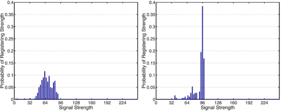
Figure 2: Samples of signal strength taken at the same positions facing opposite directions

0 32 64 96 128 160 192 224 0 0.05 0.1 0.15 0.2 0.25 0.3 0.35 0.4

Signal Strength 0 32 64 96 128 160 192 224 0 0.05 0.1 0.15 0.2 0.25 0.3 0.35 0.4

Signal Strength

Figure 3: Examples of signal strength distributions of two different base stations, measured simultaneously from one location

The local average of the signal varies slowly with the displacement. These slowßuctuations depend mostly on environmental character-istics and are known as long-term fading.

While much effort has been made to model radio signal propa-gation and attenuation in indoor environments, no single consistent model is available. During our initial experiments we took numer-ous measurements at varinumer-ous positions in our environment. Our objective was to try to see if the variables in the system could be captured with a simple theoretical model to minimize the training phase. We observed a number of interesting properties of RF sig-nals in our environment.

Orientation Matters. The authors of RADAR established a

cor-relation between orientation and measured signal strength [3, 2]. We also observed this. The laptop and the operator affect the signal in a measurable way. It is interesting to note that the presence of the operator affects signal strength and gives the omnidirectional signals some weakly directional properties. Typically the mean signal strength varies less than the statistical distribution of sig-nal strengths. In Figure 2, we give an example of two distributions sampled at the same points while facing in opposite directions.

Noise Distribution Non-Gaussian. The noise distributions at a

Þxed position were very heterogeneous as we varied the pose and base station that we sampled. In Figure 3, we show two typical examples of the signal strength at different base stations measured simultaneously at the same physical position. Several hundred sam-ples were taken in about fortyÞve seconds for these particular his-tograms. Notice that theÞrst-order properties of these distributions differ greatly from each other. In general, we have observed that distributions were asymmetric and had multiple modes. There is usually a dominant mode which often differs from the mean. We

concluded that distributions were essentially non-Gaussian. Since the noise behavior is an extremely complex physical phenomenon and explicit histograms are fairly compact, we decided that it would be better to work directly with these distributions rather than reduce the data to average values.

We found it useful to postprocess the sampled distributions by applying a small window smoothing convolution, adding a very small uniform baseline distribution and then normalizing. This is done to try to artiÞcially compensate for sampling errors and allow for a small probability of unexpected measurements in the Bayesian inference calculations that follow. These corrections pro-duced minor but noticeable improvements in the precision of the calculations.

2.3 A Bayesian Inference Algorithm

We model the world as aÞnite space ofstates

with aÞniteobservationspace

. Thesensor

modelis some learned or predicted model of the conditional prob-abilities of seeing some observationat state, in other words

. Astate vector is a probability vector (distribution)

over the various states.

Position is represented as a probability distribution over the states. The inference calculation consists of conditioning on the observations and then selecting a representative point from the re-sulting distribution.

Given a prior estimate of our state, , we can construct a new estimate of our state, ¼

, after observingby calculating the

in-dividual conditional probabilities ¼

for each using Bayes’ rule, ¼ .

(5)

This is a simple principal on which probabilistic inference schemes are built. Of course, the devil is in the details. To implement our system we made several design decisions. WeÞrst chose appro-priate state and observation spaces. This involved deciding on a sampling granularity for both spaces. We then learned the condi-tional probability distributions for plugging into the formula above.

2.3.1 Our Model

Our initial experiments and literature search indicated that a priori models of RF signal propagation would be difÞcult to set up with-out some on-site training. After verifying that simple assumptions such asÞtting analytic curves and surfaces to the means and Gaus-sians or other simple distributions to the variances provide poorÞts to sampled data, we opted for the simpler, more robust scheme of sampling the conditional probabilities directly. The reasoning for this is discussed further in Section 2.1.

We began by deÞning our state space. We chose a set of points on the map, each tuplea location and orientation on theßoor

of Duncan Hall where our experiments took place. There is no in-dication that adding an additional parameter for three-dimensional localization would be any harder, although we did no experiments to verify this. Our state spaceconsisted of a set ofpoints

.

Each observation in our observation space consisted of the mea-surements that occurred in a single scan from our base station scan-ner. Each base station scan returned a set ofbase station signal

strength measurements. Each base station could appear in the scan up to four times. We represent each observation as a vector

whereis the total number of base station signal strength

measure-ments,is the total number of unique base stations represented, is the frequency count for theth base station,represents the

base station in theth measurement and

is the signal strength of

that measurement.

In the training phase, at each point, we take an observation.

For each base station we build two histograms for that point. The

Þrst is the distribution of frequency counts over the sampled obser-vations. The second is a distribution of observed signal strengths. Based on this training, we can calculate two conditional probabili-ties.

is the probability that the frequency count for

theth base station iswhen we are at state. is

the probability that base stationhas signal strength at state

. By multiplying these conditional probabilities we obtain the

conditional probability of receiving a particular observation. For

, we compute . We note that one observation is typically enough information to decide on one’s position. However, errors in the training phase can lead to inaccuracy during localization. SigniÞcant causes of such error are subsampling and time-dependent phenomena. Subsam-pling can create a posteriori model of the noise as measured at that point. Certain measurements that occur rarely may never occur in the subsample. When the measurement occurs online, the hypoth-esis can be rejected entirely based on a conditional probability of zero for that position. We describe heuristics compensating for this difÞculty in Section 4.

After trying several possible schemes, we decided to solve a global localization problem for each observation rather than keep a

running estimate because each observation usually contains enough information to get a good guess of our position. The resulting stream of guesses can be combined in a post-processing step to create a more reÞned estimate of position. One such mechanism is described in Section 2.4.

The exact calculation proceeds as follows: before each observa-tion we choose our prior state distribuobserva-tion as the uniform distri-bution. This is a common Bayesian assumption; we assume we are lost so every position is equally likely. This provides a conserva-tive estimate of our location; any attempt to bias this initial esti-mate may inhibit accurate localization right from the start. When we make the observation, we simply use Bayes’ rule to compute

¼

, the probability distribution over the states. Then it is simply a matter of choosing appropriate candidate locations.

2.4 Sensor Fusion

We used a post-processing technique called sensor fusion to reÞne our initial location estimate. Sensor fusion is the process of com-bining multiple independent observations to obtain a more robust and precise estimate of the measured variables. We implemented aÞlter which takes the output of the inference engine as a stream of timed observations and tries to stabilize the distribution by not-ing that a person carrynot-ing a laptop typically does not move very quickly. It also takes into account some probability of error on the part of the inference engine.

We model a moving operator trying to track her position as a hidden Markov model (HMM). We use a moreÞnely discretized state space than the Bayesian inference engine and try to interpolate our position out of the stream of measurements coming from the inference engine. This design decision was made after noticing that na¨õve averaging of the inference engine’s output produced results with twice the precision we expected for points where we had not taken any training samples.

For our purposes, an HMM is a set of states ,

a set of observations, a conditional probability

function , and a transition probability matrix.

Each state and each observation is a point.

The transition probability matrix semantics describe how the sys-tem being modeled evolves with time. In this case, it describes how a person travels through the state space. If is a probability dis-tribution over, then

¼

is the probability distribution after

some discrete time step. The idea is that the random state change occurs “hidden” from the observer. We generate the transitional probability matrixusing a relatively simple heuristic, that people

don’t travel too fast or change directions too frequently.

The observation functionhas semantics identical to

observa-tion in the Bayesian inference of posiobserva-tion. ,

the probability of observingwhile at. The conditional

proba-bility functionis also deÞned using a relatively simple heuristic;

smaller distances from an observation to a given state lead to higher probabilities of making that observation at that state. As each ob-servation arrives,is used to update the probability of being in a

given state in, and thenis used to transition states. If

accu-rately models the behavior of the inference engine andaccurately

models the behavior of a person transitioning from state to state, the sensor fusion will have superior results to Bayesian inference alone.

3. Results

In this Section we describe several experiments which try to ob-jectively measure the precision and reliability of our system. We

(6)

0 1 2 3 4 5 6 7 8 9 10 0.25 0.5 0.75 1 Cumulative Probability Error (m)

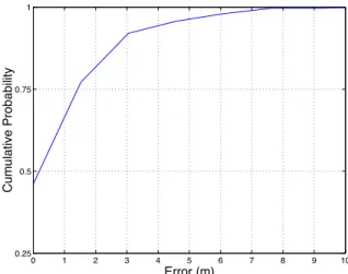
Figure 4: Bulk cumulative error distribution for 1307 packets over 22 poses in a hallway localized using the position of max-imum probability as calculated by direct application of Bayes’ rule. 0 1 2 3 4 5 6 7 8 9 10 0.25 0.5 0.75 1 Cumulative Probability Error (m)

Figure 5: Bulk cumulative error distribution for 1465 packets over 22 poses in a hallway localized using the position of maxi-mum probability as calculated by merging distributions over a one second window.

Þrst present the results for static localization. We then describe the results for user tracking using sensor fusion.

Our system was trained by taking samples at various points in the world, as discussed in Section 2.3.1. The amount of data taken at each point is varied adaptively according to a simple heuristic which measures the rate of convergence to a stable distribution. Once the sampled distribution at each visible base station had con-verged beyond a threshold, we halt the process. This allowed us to adaptively determine how much sampling is necessary as a func-tion of variafunc-tion in the signal. In our case, usual sampling times ranged from ten seconds to about a minute.

3.1 Static Localization in a Hallway

This subsection describes experiments executed in hallway 1 of our test area (see Figure 1), which was sampled in two different orien-tations at every 5 feet. The purpose of this was to test the precision of the Bayesian inference localizer. Timed tests occurred at various

positions and at both orientations in the hallway and bulk statistics were calculated.

The training data was taken by two different operators, with each operator training the localizer in one of the two directions. All experiments were executed by a third operator. The purpose of this was to demonstrate a degree of operator-independence.

Basic Bayesian Inference. Using the algorithm described in

Section 2.3, we measured a total of 1307 packets over both orienta-tions on 11 different posiorienta-tions. The posiorienta-tions were spread every 10 feet to be exhaustive. The algorithm reported positions back dis-cretized to 5 feet. In Figure 4, we show the cumulative probability of obtaining error less than a given distance. We have observed that error is withinmeters with probability.

Simple Averaging Improves Results. In the second

experi-ment, we post-processed the probability distributions computed by Bayesian inference with the following simplistic sensor fusion transform: for each, whereis the number of states,

¼

.

is the prior distribution on position, ¼

is the revised distribu-tion,is the probability distribution computed with the algorithm

of Section 2.3 and are small constants representing artiÞ

-cial uniform distributions. The resulting distribution ¼

needs to be normalized after this calculation.

This simple calculation improved our results signiÞcantly and is usable as a tracker. Our results are summarized in Figure 5. The measured error was within 1.5 meters with probability. This is

anpercent improvement over the rawÞlter. As a tracker, we

ob-served that it lagged behind the actual position and we attempted to improve our results by using more sophisticated methods described in the next section.

Operator Bias. The above results, with training and

experiment-ing done by different people, tend to suggest that operator bias tends to be less signiÞcant than sampling error and time dependent effects. In particular, operator bias is not so signiÞcant as to cause the results to be unstable.

3.2 Experiments with Tracking

We attempted to improve these results by implementing a more so-phisticated sensor fusion based on a hidden Markov model (HMM), as described in Section 2.4. We then walked round-trips of the four hallways in our test area, shown on the map in Figure 1, tracking our current position and recording the output of both the static lo-calization as described in Section 3.1 and the sensor fusion. The results are shown in Figures 6 through 9.

For hallways 1 and 2, sensor fusion increased byand,

respectively, the probability of error less than one meter. The traces show that while static localization is good at tracking, sensor fusion improves the results by effectively ignoring outliers. See Figures 6 and 7 for the results on these hallways.

The results for hallway 4 was somewhat more disappointing. The probability of error less that one meter was increased by a scant

%. Sensor fusion loosely tracked actual movement, but the signal

from the static localizer was too noisy to allow for the level of ac-curacy achieved on hallways 1 and 2. We attributed this noise to the fact that this hallway was open. See Figure 8 for the results on this hallway.

The worst result was on hallway 3, which is entirely open on one side. The probability of error less than one meter actually went down by%. As seen in Figure 9, the static localizer for the most

(7)

0 10 20 30 40 50 60 70 80 0 100 200 300 400 500 600 Time Position Actual Position Sensor Fusion Static Localization 0 1 2 3 4 5 6 7 8 0 0.1 0.2 0.3 0.4 0.5 0.6 0.7 0.8 0.9 1 Error (m) Cumulative Probability Sensor Fusion Static Localization

Figure 6: Tracking a round-trip walk of hallway 1 in our test area (see Figure 1 the building map). Measured error for the track,

shown on the right graph, is within one meter with probability, an improvement ofover static localization. This

improve-ment is illustrated in the actual tracking performance, shown in the left graph. Position in the left graph is measured in pixels on our map; 50 pixels is approximately equal to 3 meters.

0 10 20 30 40 50 60 70 0 100 200 300 400 500 600 Time Position Actual Position Sensor Fusion Static Localization 0 1 2 3 4 5 6 7 8 9 10 0 0.1 0.2 0.3 0.4 0.5 0.6 0.7 0.8 0.9 1 Error (m) Cumulative Probability Sensor Fusion Static Localization

Figure 7: Tracking a round-trip walk of hallway 2 in our test area (see Figure 1 the building map). Measured error for the track,

shown on the right graph, is within one meter with probability, an improvement ofover static localization. This improvement

is illustrated in the actual tracking performance, shown in the left graph. Position in the left graph is measured in pixels on our map; 50 pixels is approximately equal to 3 meters.

part tended to choose either an endpoint or one of two particular points in the middle of the hallway. This was caused in part by the fact that this hallway is exposed to a large open area, diluting the signal. In addition, all base stations are some distance off to a side, which means our distance (and thus the signal strength) to these base stations does not vary much as we walk the hallway.

Note that the conditional probability function and transition probability matrix we used to initialize the hidden Markov model were generated based on Gaussian distributions. While these were goodÞts for hallways 1 and 2, they failed to model the noisiness of the static localizer on hallways 3 and 4. A conditional probabil-ity function trained to the actual points would likely provide better results.

4. Discussion

The probabilistic robotics-based location-support method with RF-signals that has been described in this paper efÞciently reports and tracks the two dimensional position and orientation of a mobile wireless device in an indoor environment. While this is not the

Þrst application of probabilistic techniques to theÞeld of location-aware computing, it is one of theÞrst application of such techniques for wireless computing in an indoor environment with commodity hardware. This and the rigorous application of state-of-the-art tech-niques borrowed from robot localization are the main contributions of this paper. Our work provides a strong indication that localiza-tion can be achieved with widely available and inexpensive 802.11b wireless Ethernet hardware. This section will discuss some advan-tages and disadvanadvan-tages of our techniques.

(8)

0 10 20 30 40 50 0 50 100 150 200 250 300 Time Position Actual Position Sensor Fusion Static Localization 0 1 2 3 4 5 6 7 8 9 10 0 0.1 0.2 0.3 0.4 0.5 0.6 0.7 0.8 0.9 1 Error (m) Cumulative Probability Sensor Fusion Static Localization

Figure 8: Tracking a round-trip walk of hallway 4 in our test area (see Figure 1 the building map). While sensor fusion provided some improvement, it was not signiÞcant. As shown in the left graph, when static localization was signiÞcantly off, so was sensor fusion, but when static localization appears to track actual movement, sensor fusion is surprisingly accurate despite the noise. Position in the left graph is measured in pixels on our map; 50 pixels is approximately equal to 3 meters.

0 10 20 30 40 50 0 50 100 150 200 250 300 Time Position Actual Position Sensor Fusion Static Localization 0 1 2 3 4 5 6 7 8 9 10 11 12 13 14 0 0.1 0.2 0.3 0.4 0.5 0.6 0.7 0.8 0.9 1 Error (m) Cumulative Probability Sensor Fusion Static Localization

Figure 9: Tracking a round-trip walk of hallway 3 in our test area (see Figure 1 the building map). Sensor fusion did not provide a signiÞcant improvement in error, and at times increased error, as shown in the right graph. However, as shown in the left graph, the raw data was already extremely noisy in this case. Position in the left graph is measured in pixels on our map; 50 pixels is approximately equal to 3 meters.

4.1 Advantages

Accuracy. The accuracy of RF based localization is substantially

improved in our experimental setup over the reported resolution and accuracy of similar previous efforts. RADAR [3, 2] exhibited a median resolution in the range of 2 to 3 meters. Our results indicate that we can get a resolution of less thanmeters with an accuracy % given suitable base station layout. At a coarse resolution, we

are very reliable. This is because noise texture varies signiÞcantly over relatively large distances, especially when there are interven-ing obstacles. Inside a room, there are ambiguities in sensinterven-ing that lead to error. In all of our experiments, we never observed coarse granularity errors except at corners and doorways where the opera-tor is transitioning from one area to another. Our sensor fusion can

improve precision while tracking a moving object by interpolating between sampled points and taking advantage of spatial continuity assumptions to probabilistically reject outliers.

Orientation. Our method explicitly tries to solve for orientation.

This is necessary since as we and others [3, 2] have observed ori-entation is a factor in observed signal strength. In fact, our exper-iments show that orientation can be coarsely determined by signal strength variations which shows the correlation is often highly non-trivial. By explicitly modeling position and direction, we greatly improve static localization and sensor fusion although orientation determination tended to be much noisier than position. This allows us to overcome difÞculties that weakened the applicability of the results of RADAR. On the other hand, we strongly believe the

(9)

vari-ations in signal due to orientation are not sufÞciently large to ever obtain more than a coarse estimate of direction without employing differential methods with a moving observer.

Cost and Complexity. The advantage of using wireless Ethernet

RF signals for localization is that the sensor doubles as a commu-nication device. The infrastructure for such networks already ex-ists in many real-world environments and consequently, for many mobile devices, this sort of localization can be implemented as a software-only solution. This is an attractive option for a number of real-world applications.

Extensibility and Scalability. The methods we use are very

gen-eral and experiments with a variety of robot localization applica-tions have proven the approach very adaptable. In particular, the framework can be used with other sensors. For example, by using ultrasound sensors such as those used in Cricket [32], we estimate that we could increase our precision to the order of twenty cen-timeters. This increase in precision is alluded to by the authors of Cricket as a point of future work when they suggest employing KalmanÞlters [32, 33].

We believe that localization with wireless Ethernet signal strengths scales well into much larger arenas than our experimental test-bed with the caveat that the layout of base stations should be non-pathological. Our evidence for this comes from robot local-ization and the experimental observation that, at room granularity, signal strength distributions differ greatly.

The particular algorithms we present do not scale if used ver-batim. The computational cost of localization in the algorithms we present grows as a linear (Bayesian) or quadratic (sensor fu-sion) function of the number of possible poses. The vectors and matrices involved however are almost always very sparse. The typ-ical approach in larger cases is to proceed by Monte Carlo (MC) integration of the conditional probability distributions [37]. The computational efÞciency of MC is validated by the successful im-plementation of these algorithms for mobile robots with severely restricted computational power such as the Sony AIBO robot [30].

Privacy and Security. It has been claimed in previous works,

such as Cricket [32, 33], that a location support system can be im-plemented in such a way as to localize a user only if she is willing to be localized. This assertion, though, breaks down if the mobile device is not passive, for example if it is using an active localiza-tion scheme or is using wireless networking to communicate. This raises issues of anonymity, privacy, and security. Third-party ob-servers using conventional hardware could conceivably determine the position of a mobile device broadcasting on a wireless Ethernet network without the device’s knowledge or permission. Likewise, a network administrator could use the network to track users by having the base stations monitor observed signal strengths.

4.2 Disadvantages

Environment Dependence. Every localization system is

ham-pered by a dependence on the environment it is executed in. In our case, we noticed that some of the areas we tested, notably hall-way 3, provided lower accuracy than other areas. The placement of the base stations, the materials in the building, and the building’s geometry can affect the difÞculty of localizing at a given point. A more worrisome challenge is the variation induced by people ab-sorbing RF signals and other dynamic effects. When working with 2.4 GHz RF signals both static and dynamic environmental condi-tions can be difÞcult to predict and have complex behaviors. We believe that continued research on heuristics for coping with these

problems either by judicious placement of base stations or by im-provements in the localization algorithm can produce usable results for many applications even in the face of such environmentalßux.

Training. The complexity of indoor RF signal propagation is

avoided by building a sensor map. The time spent training these maps is a limitation of all localization approaches using a sampling technique for generating maps. As it is, maps were built by mark-ing the workspace and takmark-ing measurements at each point. Fur-ther automation might be necessary to facilitate deployment of an approach in this spirit. In mobile robotics, map building and ex-ploration for such localization approaches is an important area of research. By augmenting the operator with some extra sensors, for example an accelerometer and magnetic compass to use for dead reckoning, a walk around the building could be used together with a mapping algorithm [36] to automate training further.

4.3 Future Work

This work can be extended in a number of different directions. Most directly, we could expand the experimental area, possibly considering multipleßoors and signiÞcant amounts of area within rooms. There are also a number of algorithmic aspects of mobile node location tracking that could be explored.

Compensating for dynamic occlusion in robotics localization is a studied problem but is also quite difÞcult. Many approaches try to predict some variables describing dynamic state. For example, a tour-guide museum robot needs to model the motion of people in the museum to avoid collisions [4]. Multi-robot, collaborative lo-calization is another branch of lolo-calization research [14]. Much of the work in this area is relevant to collaborative localization in an ad hoc wireless network. This is a fascinating problem which mixes issues in protocol design and communication with uncertainty and localization. Relative and differential techniques may be of use in combating variations that occur due to environmental effects. For example, landmark based navigation operates using only the angle of deßection to the base station [1]. Pursuit-evasion robotics stud-ies the problem of capturing an active evader under various sensing and environmental constraints. In location-aware security for wire-less networks, studying how to intercept a moving intruder under various assumptions about sensing could be an interesting and chal-lenging problem.

5. Related Work

5.1 Location Aware Computing

Many other systems have been built to support indoor localization. These systems vary in many parameters, such as the sensors, the cost, the required hardware, the infrastructure and the resolution in time and space [21].

The AT&T Cambridge Laboratory’s Active Badge location sys-tem [38] and the more recent Active Bat syssys-tem [39] are two of theÞrst systems in theÞeld. Active Badge uses diffuse IR technol-ogy while Active Bat uses an ultrasound time-of-ßight technique to provide accurate physical positioning. Users and objects have to carry Active Bat tags, emitting an ultrasonic pulse to a grid of ceiling-mounted receivers and a simultaneous “reset” signal over a radio link. Each ceiling sensor measures the time interval from reset to ultrasonic pulse arrival and computes its distance from the Bat.

The Cricket Location Support System [32, 33] also uses ultra-sound emitters and embeds low-cost receivers in the object being located. Cricket uses additional radio frequency signals to synchro-nize time measurements and to distinguish ultrasound signals that

(10)

are a result of multi-path effects. The main localization techniques that are employed in Cricket are based on triangulation relative to the beacons. Cricket trades accuracy for simpler hardware and in-frastructure. It does not require a grid of ceiling sensors withÞxed locations as in the Active Bat system but returns an estimation of the user’s position with a possible error of a four foot by four foot region, while the Active Bat has an accuracy of nine centimeters. Both of these systems provide excellent localization primitives by employing specialized hardware.

Computer vision has also been used in location support systems. Microsoft Research’s Easy Living uses stereo-vision cameras to measure three-dimensional position in a home environment [25]. Camera-based approaches are expensive in terms of hardware in-frastructure due to the cost of the camera and the computational overhead of image processing.

RF-Based Systems. The RADAR system [3, 2] uses only a

wire-less networking signal, employing nearest neighbor heuristics and other pattern recognition techniques for localization. The authors report localization accuracy of about 3 meters of their actual po-sition with aboutÞfty percent probability. They also discuss the problems of localizing in the face of multipleßoors and chang-ing environmental conditions, as well as trackchang-ing of movchang-ing users. While our work has similar design goals to RADAR, we take a very different algorithmic approach, using a probabilistic technique pop-ular in many robotics applications.

The PinPoint location system [40] is similar to RADAR, but uses expensive, proprietary base station and tag hardware to measure radio time ofßight. PinPoint’s accuracy is roughly 1 to 3 meters.

In the SpotOn system [22], special tags use radio signal atten-uation to estimate distance between tags. The aim in SpotOn is to localize wireless devices relative to one another, rather than to

Þxed base stations, allowing forad-hoc localization. The proba-bilistic framework we are proposing could also be applied in the case of ad-hoc location sensing.

A number of systems have been built using probabilistic tech-niques to determine location based on RF signal strength for cellu-lar telephone systems. Liu et al. [28] use Markov modeling and KalmanÞltering to predict when a mobile node will cross cell boundaries. Yamamoto et al. [41] use Bayesian analysis to deter-mine the absolute location of a mobile node.

RF Signal Attenuation. Much effort has been made to model

radio signal propagation in an indoor environment [17, 31]. Dif-ferent experiments in the literature have arrived at difDif-ferent distri-butions. Although each result may be justiÞable for a certain set of conditions that govern a certain set of measurements, a consis-tent model that would give a signal strength distribution under a diversiÞed set of conditions is unavailable. However, experiments with 12000 impulse response proÞles in two ofÞce buildings have shown good log-normalÞt [19]. A general empirical model [17] for indoor propagation of radio signals can be expressed as

whereis the path loss in dB at distance,

is the

known path loss at the reference distance,denotes the

expo-nent depending on the propagation environment andis the

vari-able representing uncertainty of the model. We note that decibels are a log-scale.

Based on this general formulation, many empirical models have been derived in theÞeld of indoor propagation modeling in the

wireless community. Parameteris very sensitive to the

propa-gation environment, like the type of the construction material and type of the interior [31], limiting the value of these models.

5.2 Robot Localization

Robot localization is a well-studied problem in robotics. Robot lo-calization is the process of maintaining an ongoing estimate of a robot’s location with respect to its environment, given a representa-tion of this environment and some sensing ability within the envi-ronment. The importance of this problem in the context of building reliable robot systems cannot be overstated; determining the pose (position and orientation) of the robot from physical sensors is of-ten referred to as “the most fundamental problem to providing a mobile robot with autonomous capabilities” [8]. In our case, we can consider any wireless device as a mobile robot.

If there is no a priori estimate of the robot’s location, the prob-lem is referred asglobal localization, which is a particularly chal-lenging case of localization. This is the type of problem we dis-cussed. We have no information where the wireless device is before it starts communicating with the network’s base stations. Further-more, there is the need to reÞne the estimate of the device’s pose continuously. This task is known aspose maintenance.

Sensor based localization is based on the premise that we use sensor data in conjunction with the representation of the environ-ment to produce a reÞned position estimate, such that this estimate is more likely to predict the true positions. By sensor, we mean any device which can measure attributes of the environment in a way that can be correlated to position. Typical sensors that are de-ployed in robotics are IR transmitters, ultrasound or laser proximity sensors and camera images.

Sensor fusionis another important notion in robot localization. A broad deÞnition of sensor fusion is the combination of multiple independent observations to obtain a more robust and precise esti-mate of the measured variables. This can be implemented in terms of integrating sensor readings over time or in the synthesis of mea-surements from multiple sensors. Most of the recent work in robot localization has been in improving and implementing sensor fusion for many systems.

Much progress has been made in developing localization tech-niques since the problem Þrst appeared in the literature. Dead reckoning can be used for pose maintenance, but requires some initial knowledge of location. Some of the simplest methods for global localization include landmark-based localization and trian-gulation. Probabilistic techniques, such as KalmanÞltering, and later, Bayesian analysis, were developed to addressßaws in these systems. Finally, for when a grid-based map is inappropriate to the application or environment, topological approaches have been developed.

Dead Reckoning. Perhaps the simplest approach to the pose

maintenance task is to keep track of how far the robot moves in each direction and then to sum these motions to produce a net dis-placement that can be added to an initial position estimate. Keep-ing track of how much one moves by observKeep-ing internal parameters without reference to the external world is known as dead reckoning and is usually implemented with an odometer. If onlydead reck-oningis used for position estimation, these errors are added to the absolute pose estimate and errors are accumulated. Long-term lo-calization must make reference to the external world for position correction. This involves the use of sensory data for recalibrating a robot’s sense of its own location with the environment. In some circumstances, such as the case of a wireless device that a person is moving around in space, we have no analogue of odometry.

(11)

Triangulation. Distance to known landmarks is frequently used to determine pose as this can be computed with cameras, laser range-Þnders, IR transmitters, sonar and other commonly used sen-sors. A na¨õve approach is to take three distance measurements and triangulate position. This works when the sensors are reliable and relatively noise-free but leaves several problems unaddressed. When the sensors are noisy, the calculations for triangulation be-come unstable for many positions and landmark arrangements and lead to signiÞcant loss of precision. Typically, multiple measure-ments are merged over time to try to compensate for this, however some care must be taken in choosing the method of merging or poor results will be obtained [11]. In some cases where the sensors are fairly reliable and have simple noise distributions, direct trian-gulation or triantrian-gulation with differential windowing can produce excellent results. Noisy sensors, however, complicate triangulation adding uncertainty to the results. GPS [29] is perhaps the most-used sensor based on triangulation.

Kalman Filter. In 1987, Smith and Cheeseman introduced the

use of KalmanÞlters to the problem of determining position [34]. Many systems in robot localization, since then, have been based on KalmanÞltering [16, 27, 10]. The robot’s pose estimation is main-tained as a Gaussian distribution inÊ

and sensor data from

dead reckoning and landmark observations is fused to obtain a new position distribution. This method is provably optimal when all distributions are linear but typically fails when these assumptions break down. Extended KalmanÞlters address this problem by lin-earizing the system. In practice, obtaining linearizations for many sensing systems is difÞcult and errors can propagate very quickly through the system.

Bayesian Approaches. Possibly the most powerful family of

global localization algorithms to date is based on Bayesian infer-ence, in particular Markov localization [24, 15] and Monte Carlo localization [13, 37]. These are generalizations of the KalmanÞ l-ter. These algorithms estimate posterior distributions over robot poses which are approximated by piecewise constant functions in-stead of Gaussians, enabling them to represent highly multi-modal distributions. In this way, they can be applied in the case of sensors that are non-linear and have non-Gaussian noise distributions. The accuracy of the results, however, is limited by the resolution of the approximation. Due to the very complex nature of some sensors and usually also of the environment, many systems have difÞ cul-ties modeling outliers and other artifacts. These difÞculties can be addressed by sampling the distributions of the sensor signals in the target environment and using this directly as a model, as in the case of the sensor map we built in theÞrst phase of our method. By ex-plicitly integrating the conditional probability distributions, we can obtain precise approximations of the robot’s positional distribution. This approach is both computationally tractable and effective [37]. Many excellent examples of this method exist in the literature [35]. This the approach we took in implementing localization using wire-less Ethernet, as described in Section 2.

Topological Approaches. Typically the Bayesian approach is

applied in the case when we have a grid-based representation of the environment. Another alternative for modeling the environment is with a topological map, represented as a generalized Voronoi graph [6]. Localization on the topological map is based on the fact that the robot automatically identiÞes nodes in the graph from geo-metric environmental information [26].

6. Conclusions

In this paper, we provide strong evidence that reliable localization with wireless Ethernet can be achieved. In our experiments, we can measure and track position robustly with theÞrst meter of error distributed within a standard deviation. We used the Intersil Prism2 chipset for our wireless Ethernet cards and Apple AirPort base sta-tions, both readily available and inexpensive hardware. The build-ing we operated in had fairly complicated geometry and the base stations were laid out more than a year before we began our work. The methods we employed were general methods from robotics and followed the Bayesian approach to localization. These methods were readily adaptable to the problem at hand and can be applied to other location problems that might arise in mobile computing.

7. Acknowledgements

The authors would like to thank Moez Abdel-Gawad and Skye Schell for their help with taking measurements. They would also like to thank Dave Johnson for his advice and comments. Thanks also to Scott Crosby and to the anonymous MOBICOM’02 review-ers for their comments.

Andrew Ladd is partially supported by FCAR 70577, by NSF-IRI-970228 and a Whitaker grant. Kostas Bekris is partially sup-ported by IRI-970228. Algis Rudys is supsup-ported by NSF-CCR-9985332. Dan Wallach is supported by an NSF Career Award CCR-9985332, an NSF Special Projects Award ANI-9979465, and a Texas ATP award. Lydia Kavraki is supported by NSF Career Award IRI-970228, a Whitaker grant, a Texas ATP award and a Sloan Fellowship.

8. References

[1] A. A. Argyros, K. E. Bekris, and S. C. Orphanoudakis. Robot homing based on corner tracking in a sequence of a panoramic images. InProc. of the IEEE Computer Society Conference on Computer Vision and Pattern Recogntion (CVPR 2001), volume 2, pages 3–10, Kauai, Hawaii, Dec. 2001.

[2] P. Bahl and V. N. Padmanabhan. Enhancements to the RADAR user location and tracking system. Technical Report MSR-TR-2000-12, Microsoft Research, Feb. 2000.

[3] P. Bahl and V. N. Padmanabhan. RADAR: An in-building RF-based user location and tracking system. InProc. of IEEE In-focom 2000, volume 2, pages 775–784, Tel Aviv, Israel, Mar. 2000.

[4] W. Burgard, A. Cremers, D. Fox, D. Hahnel, G. Lakemeyer, D. Schulz, W. Steiner, and S. Thrun. The interactive museum tour-guide robot. InProc. of the Fifteenth National Confer-ence on ArtiÞcial Intelligence (AAAI-98), Madison, Wiscon-sin, July 1998. Outstanding paper award.

[5] A. Chakraborty. A distributed architecture for mobile, location-dependent applications. Master’s thesis, Mas-sachusetts Institute of Technology, May 2000.

[6] H. Choset and K. Nagatani. Topological simultaneous lo-calization and mapping (SLAM): Toward exact lolo-calization without explicit localization.IEEE Transactions on Robotics and Automation, 17(2):125–137, Apr. 2001.

[7] T. W. Christ and P. A. Godwin. A prison guard duress alarm location system. InProc. IEEE International Carnahan Con-ference on Security Technology, Oct. 1993.

[8] I. Cox. Blanche - an experiment in guidance and navigation of an autonomous robot vehicle.IEEE Transactions on Robotics and Automation, 7(2):193–204, 1991.

(12)

[9] T. Cutler. Wireless Ethernet and how to use it.The Online Industrial Ethernet Book, Issue 5, 1999.

[10] A. J. Davison and N. Kita. 3D simultaneous localization and map-building using active vision for a robot moving on un-dulating terrain. InProc. IEEE Computer Society Conference on Computer Vision and Pattern Recognition (CVPR 2001), volume 1, pages 384–391, Kauai, Hawaii, Dec. 2001. [11] G. Dudek and M. Jenkins.Computational Principles of

Mo-bile Robotics. Cambridge University Press, 2000.

[12] Federal Communcations Commission Report and Order 96-264: Revision of the commission’s rules to ensure compat-ibility with Enhanced 911 emergency calling systems, July 1996. http://www.fcc.gov/Bureaus/Wireless/ Orders/1996/fcc96264.txt.

[13] D. Fox, W. Burgard, F. Dellaert, and S. Thrun. Monte Carlo localization: EfÞcient position estimation for mobile robots. InProc. of the Sixteenth National Conference on ArtiÞcial In-telligence (AAAI-99), pages 343–349, Orlando, Florida, 1999. [14] D. Fox, W. Burgard, H. Kruppa, and S. Thrun. A proba-bilistic approach to collaborative multi-robot localization. Au-tonomous Robots, 8(3):325–344, June 2000.

[15] D. Fox, W. Burgard, and S. Thrun. Markov localization for mobile robots in dynamic environments.Journal of ArtiÞcial Intelligence Research, (JAIR), 11:391–427, Nov. 1999. [16] J. Guivant and E. Nebot. Optimization of the simultaneous

localization and map building algorithm for real time imple-mentation. Journal of Robotics Research, 17(10):565–583, 2000.

[17] P. Harley. Short distance attenuation measurements at 900MHz and 1.8GHz using low antenna heights for micro-cells. IEEE Journal on Selected Areas in Communications (JSAC), 7(1):5–11, Jan. 1989.

[18] A. Harter, A. Hopper, P. Steggles, A. Ward, and P. Webster. The anatomy of a context-aware application. InProc. of the 5th Annual ACM/IEEE International Conference on Mobile Computing and Networking (MOBICOM 1999), pages 59–68, Seattle, WA, Aug. 1999.

[19] H. Hashemi. Impulse response modeling of indoor radio prop-agation channels.IEEE Journal on Selected Areas in Commu-nications (JSAC), 11:967–978, Sept. 1993.

[20] H. Hashemi. The indoor radio propagation channel.Proc. of the IEEE, 81(7):943–968, July 1993.

[21] J. Hightower and G. Borriello. Location systems for ubiqui-tous computing.IEEE Computer, 34(8):57–66, Aug. 2001. [22] J. Hightower, R. Want, and G. Borriello. SpotON: An indoor

3D location sensing technology based on RF signal strength. Technical Report UW CSE 00-02-02, University of Washing-ton, Department of Computer Science and Engineering, Seat-tle, WA, Feb. 2000.

[23] Institute of Electrical and Electronics Engineers, Inc. ANSI/IEEE Standard 802.11: Wireless LAN Medium Access Control (MAC) and Physical Layer (PHY) SpeciÞcations, 1999.

[24] K. Konolige and K. Chou. Markov localization using corre-lation. InProc. of the Seventeenth International Joint Con-ference on ArtiÞcial Intelligence (IJCAI), pages 1154–1159, Seattle, Washington, Aug. 1999.

[25] J. Krumm, S. Harris, B. Meyers, B. Brumitt, M. Hale, and S. Shafer. Multi-camera multi-person tracking for EasyLiv-ing. InThird IEEE International Workshop on Visual Surveil-lance, Dublin, July 2000.

[26] B. Kuipers and Y. T. Byan. A robot exploration and mapping strategy based on a semantic hierarcy of spatial representa-tions.Journal on Robotics and Automatic Systems, 8:47–63, 1991.

[27] J. F. Leonard and H. Durrant-Whyte. Mobile robot local-ization by tracking geometric beacons. IEEE Transactions Robotics and Automations, 7(3):376–382, June 1991. [28] T. Liu, P. Bahl, and I. Chlamtac. Mobility modeling,

loca-tion tracking, and trajectory predicloca-tion in wireless ATM net-works.IEEE Journal on Selected Areas in Communications, 16(6):922–936, Aug. 1998.

[29] T. Logsdon.Understanding the Navstar: GPS, GIS and IVHS. Second edition. Van Nostrand Reinhold, New York, 1995. [30] G. Marceau. The McGill’s RedDogs legged league system.

Robocup 2000, pages 627–630, 2000.

[31] A. Neskovic, N. Nescovic, and G. Paunovic. Modern ap-proaches in modeling of mobile radio systems propagation environment.IEEE Communications Surveys, Third Quarter 2000.

[32] N. Priyantha, A. Chakraborty, and H. Balakrishman. The Cricket location support system. InProc. of the 6th Annual ACM/IEEE International Conference on Mobile Computing and Networking (MOBICOM 2000), pages 32–43, Boston, MA, Aug. 2000.

[33] N. Priyantha, A. Miu, H. Balakrishman, and S. Teller. The Cricket compass for context-aware mobile applications. In Proc. of the 7th Annual ACM/IEEE International Conference on Mobile Computing and Networking (MOBICOM 2000), pages 1–14, Rome, Italy, July 2001.

[34] R. Smith and P. Cheeseman. On the representation of spatial uncertainty.Journal of Robotics Research, 5(4):56–68, 1987. [35] S. Thrun. Probabilistic algorithms in robotics.AI Magazine,

21(4):93–109, 2000.

[36] S. Thrun, W. Burgard, and D. Fox. A probabilistic approach to concurrent mapping and localization for mobile robots. Ma-chine Learning, 31(1-3):29–53, 1998.

[37] S. Thrun, D. Fox, W. Burgard, and F. Dellaert. Robust Monte Carlo localization for mobile robots. ArtiÞcial Intelligence, 101:99–141, 2000.

[38] R. Want, A. Hopper, V. Falco, and J. Gibbons. The Active Badge location system. ACM Transactions on Information Systems, 10:91–102, Jan. 1992.

[39] A. Ward, A. Jones, and A. Hopper. A new location tech-nique for the active ofÞce.IEEE Personal Communications, 4(5):42–47, Oct. 1997.

[40] J. Werb and C. Lanzl. Designing a positioning system forÞ nd-ing thnd-ings and people indoors.IEEE Spectrum, 35(9):71–78, Sept. 1998.

[41] R. Yamamoto, H. Matsutani, H. Matsuki, T. Oono, and H. Ohtsuka. Position location technologies using signal strength in cellular systems. In Proc. of the 53rd IEEE Ve-hicular Technology Conference, May 2001.

Robotics-Based Location Sensing using Wireless Ethernet