15-441: Computer Networks Project 3: Video CDN

(1)

15-441: Computer Networks

Project 3: Video CDN

Lead TA: Titouan Rigoudy <[email protected]>

Assigned: 11/7/14

Checkpoint 1 due: 11/21/14 (11:59 PM) Final version due: 12/5/14 (11:59 PM)

1 Overview

In this project you will explore how video content distribution networks (CDNs) work. In particular, you will implement adaptive bitrate selection, DNS load balancing, and a very small subset of OSPF (which your DNS server will use to decide which server is closest to a given client).

1.1 In the Real World

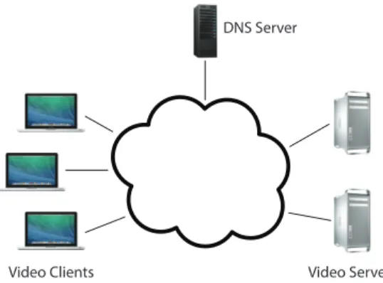
Figure 1 depicts (at a high level) what this system looks like in the real world. Clients trying to stream a video first issue a DNS query to resolve the service’s domain name to an IP address for one of the CDN’s content servers. The CDN’s authoritative DNS server selects the “best” content server for each particular client based on (1) the client’s IP address (from which it learns the client’s geographic location) and (2) current load on the content servers (which the servers periodically report to the DNS server).

Once the client has the IP address for one of the content servers, it begins requesting chunks of the video the user requested. The video is encoded at multiple bitrates; as the client player receives video data, it calculates the throughput of the transfer and requests the highest bitrate the connection can support.

1.2 Your System

Implementing an entire CDN is clearly a tall order, so let’s simplify things. First, your entire system will run on one host; we’re providing a network simulator (described in §4) that will allow you to run several processes with arbitrary IP addresses on one machine. Our simulator also allows you to assign arbitrary link characteristics (bandwidth and latency) to each pair of “endhosts” (processes). For this project, you will do your development and testing using a virtual machine we provide (§4).

(2)

Video Clients Video Servers DNS Server

Figure 1: In the real world...

Apache Apache

...

Proxy Proxy

...

Browser Browser

...

DNS

Figure 2: Your system. Figure 3: System overview.

Figure 2 shows the pieces of the system; those shaded in gray will be written by you. Browser. You’ll use an off-the-shelf web browser to play videos served by your CDN (via your proxy).

Proxy. Rather than modify the video player itself, you will implement adaptive bitrate selection in an HTTP proxy. The player requests chunks with standard HTTP GET requests; your proxy will intercept these and modify them to retrieve whichever bitrate your algorithm deems appropriate. To simulate multiple clients, you will launch multiple instances of your proxy. More detail in §2.

Web Server. Video content will be served from an off-the-shelf web server (Apache). As with the proxy, you will run multiple instances of Apache on different fake IP addresses to simulate a CDN with several content servers. More detail in §4.

DNS Server. You will implement a simple DNS (supporting only a small portion of actual DNS functionality). Your server will respond to each request with the “best” server for that particular client. More detail in §3.

2 Video Bitrate Adaptation

Many video players monitor how quickly they receive data from the server and use this throughput value to request better or lower quality encodings of the video, aiming to stream the highest quality encoding that the connection can handle. Rather than modifying an existing video client to perform bitrate adaptation, you will implement this functionality in an HTTP proxy through which your browser will direct requests.

(3)

2.1 Requirements

Checkpoint 1: The first checkpoint is all about bitrate adaptation. There are two pieces: (1) Implement your proxy. Your proxy should calculate the throughput it receives from the video server and select the best bitrate for the connection. See §2.2 for details.

(2) Explore the behavior of your proxy. Once your proxy is working, launch two instances of it on the “dumbbell” topology (topo1) we provide. Running the dumbbell topology will also create two servers (listening on the IP addresses in topo1.servers); you should direct one proxy to each server. Now:

1. Start playing the video through each proxy.

2. Run the topo1 events file and direct netsim.pyto generate a log file: ./netsim.py -l

<log-file> ../topos/topo1 run

3. After 1 minute, stop video playback and kill the proxies.

4. Gather the netsim log file and the log files from your proxy and use them to generate plots for link utilization, fairness, and smoothness. Use the provided grapher.pyscript to do this: ./grapher.py <netsim-log> <proxy-1-log> <proxy-2-log>

Repeat these steps forα= 0.1,α= 0.5,α= 0.9 (see §2.2.1). Compile your 9 plots, labelled clearly, into a single PDF namedwriteup.pdf, along with a brief (1-3 paragraphs) discussion of the tradeoffs you make as you vary α. We’re not looking for a thorough, extensive study, just general observations. For checkpoint 1 we’re only giving completion points for your writeup, so it’s okay if it’s still a bit preliminary.

2.2 Implementation Details

You are implementing a simple HTTP proxy. It accepts connections from web browsers, modifies video chunk requests as described below, resolves the web server’s DNS name (part of the HTTP request), opens a connection with the resulting IP address, and forwards the modified request to the server. Any data (the video chunks) returned by the server should be forwarded, unmodified, to the browser.

DNS resolving is checkpoint 2, so for checkpoint 1 simply point each proxy to a static server IP via a command line argument. The proxy should “resolve” every DNS name to that IP.

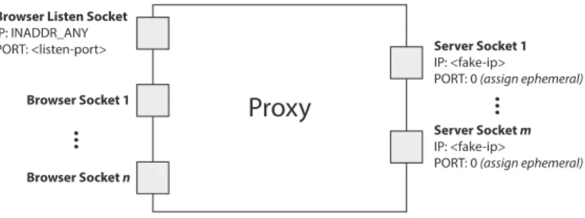
Your proxy should listen for connections from a browser on any IP address on the port specified as a command line argument (see below). When it connects to a server, it should first bind the socket to the fake IP address specified on the command line (note that this is somewhat atypical: you do not ordinarilybind()a client socket before connecting). Figure 4 depicts this. This is required by our network simulation architecture.

Your proxy should accept multiple concurrent connections usingselect(), as in project 1. It is fine to re-use select() and HTTP parsing code from project 1.

(4)

Proxy

Browser Listen Socket IP: INADDR_ANY PORT: <listen-port> Browser Socket 1 Browser Socket _n

...

Server Socket 1 IP: <fake-ip>

PORT: 0 (assign ephemeral)

Server Socket _m IP: <fake-ip>

PORT: 0 (assign ephemeral)

...

Figure 4: Your proxy should listen for browser connections on INADDR ANY _{on the port specified on the}

command line. It should then connect to web servers on sockets that have been bound to the proxy’s fake IP address (also specified on the command line).

2.2.1 Throughput Calculation

Your proxy could estimate each stream’s throughput once per chunk as follows. Note the start time,ts, of each chunk request (i.e., includetime.hand save a timestamp using time()

when your proxy receives a request from the player). Save another timestamp,tf, when you

have finished receiving the chunk from the server. Now, given the size of the chunk, B, you can compute the throughput, T, your proxy saw for this chunk:

T = B

tf −ts

To smooth your throughput estimation, your proxy should use an exponentially-weighted moving average (EWMA). Every time you make a new measurement (Tnew), update your

current throughput estimate as follows:

Tcurrent =αTnew+ (1−α)Tcurrent (1)

The constant 0 ≤ α ≤ 1 controls the tradeoff between a smooth throughput estimate (α closer to 0) and one that reacts quickly to changes (α closer to 1). You will control α via a command line argument. When a new stream starts, set Tcurrent to the lowest available

bitrate for that video. 2.2.2 Choosing a Bitrate

Once your proxy has calculated the connection’s current throughput, it should select the highest offered bitrate the connection can support. For this project, we say a connection can support a bitrate if the average throughput is at least 1.5 times the bitrate. For example, before your proxy should request chunks encoded at 1000 Kbps, its current throughput estimate should be at least 1.5 Mbps.

Your proxy should learn which bitrates are available for a given video by parsing the manifest file (the “.f4m” initially requested at the beginning of the stream). The manifest

(5)

is encoded in XML; each encoding of the video is described by a <media> element, whose

bitrate attribute you should find.

Your proxy replaces each chunk request with a request for the same chunk at the selected bitrate (in Kbps) by modifying the HTTP request’s Request-URI. Video chunk URIs are structured as follows:

/path/to/video/<bitrate>Seq<num>-Frag<num>

For example, suppose the player requests fragment 3 of chunk 2 of the video Big Buck Bunny at 500 Kbps:

/path/to/video/500Seg2-Frag3

To switch to a higher bitrate, e.g., 1000 Kbps, the proxy should modify the URI like this:

/path/to/video/1000Seg2-Frag3

IMPORTANT: When the video player requests big buck bunny.f4m, you should instead returnbig buck bunny nolist.f4m. This file does not list the available bitrates, preventing the video player from attempting its own bitrate adaptation. You proxy should, however, fetch big buck bunny.f4m for itself (i.e., don’t return it to the client) so you can parse the list of available encodings as described above.

2.2.3 Logging

We require that your proxy create a log of its activity in a very particular format. After each request, it should append the following line to the log:

time The current time in seconds since the epoch.

duration A floating point number representing the number of seconds it took to download this chunk from the server to the proxy.

tput The throughput you measured for the current chunk in Kbps.

avg-tput Your current EWMA throughput estimate in Kbps.

bitrate The bitrate your proxy requested for this chunk in Kbps.

server-ip The IP address of the server to which the proxy forwarded this request.

chunkname The name of the file your proxy requested from the server (that is, the modified file name in the modified HTTP GET message).

(6)

2.2.4 Running the Proxy

By running make in the root of your submission directory, we should be able to create an executable called proxy, which should be invoked as follows, even if not all arguments are functional at the first checkpoint:

./proxy <log> <alpha> <listen-port> <fake-ip> <dns-ip> <dns-port>

[<www-ip>]

log The file path to which you should log the messages described in §2.2.3.

alpha A float in the range [0, 1]. Uses this as the coefficient in your EWMA throughput estimate (Equation 1).

listen-port The TCP port your proxy should listen on for accepting connections from your browser.

fake-ip Your proxy should bind to this IP address for outbound connections to the web servers. You shouldnot bind your browser listen socket to this IP address — bind that socket to INADDR ANY.

dns-ip IP address of the DNS server.

dns-port UDP port DNS server listens on.

www-ip Your proxy should accept an optional argument specifying the IP address of the web server from which it should request video chunks. If this argument is not present, your proxy should obtain the web server’s IP address by querying your DNS server for the name video.cs.cmu.edu.

To play a video through your proxy, point a browser on your VM to the URL

http://localhost:<listen-port>/index.html. (You can also configure VirtualBox’s port forwarding to send traffic from<listen-port>on the host machine to<listen-port> on your VM; this way you can play the video from your own web browser.)

3 DNS Load Balancing

To spread the load of serving videos among a group of servers, most CDNs perform some kind of load balancing. A common technique is to configure the CDN’s authoritative DNS server to resolve a single domain name to one out of a set of IP addresses belonging to replicated content servers. The DNS server can use various strategies to spread the load, e.g., round-robin, shortest geographic distance, or current server load (which requires servers to periodically report their statuses to the DNS server).

(7)

3.1 Requirements

You will write a simple DNS server that implements load balancing two different ways: round-robin and geographic distance.

Checkpoint 2: DNS load balancing comes into play at the second checkpoint. You must implement the two load balancing strategies described below. In order for you proxy to be able to query your DNS server, you must also write an accompanying DNS resolution library (see §3.2 for details).

(1) Round robin. First, implement a simple round-robin based DNS load balancer. Your DNS process should take as input a list of video server IP addresses (the topology’s.servers

file — §4.2) on the command line (§3.2); it responds to each request to resolve the name

video.cs.cmu.eduby returning the next IP address in the list, cycling back to the beginning when the list is exhausted.

(2) Geographic distance. Next you’ll make your DNS server somewhat more sophisticated — it must return the closest video server to the client based on the client’s IP address. In the real world, this would be done by querying a database mapping IP prefixes to geographic locations. In your implementation, you will pretend that a link state routing protocol (e.g., OSPF) is used Internet-wide and that your DNS server participates in it. Your DNS server must process link state advertisements (LSAs), build a graph of the entire network, and run Dijkstra’s shortest path algorithm on the graph to determine the closest video server for a given client.

You do not need to implement LSA flooding. We will provide you with a file containing a list of LSAs which your server would have received had you actually implemented LSA flooding. The file contains one LSA per line, formatted as follows:

sender The IP address of the node that originated this LSA.

sequence number An integer allowing you to order the LSAs from a given sender. Each node sends multiple LSAs; you should accept only the most recent (even if they arrive out of order). You may assume sequence numbers don’t wrap back to zero within the LSA file and that nodes in the network never reboot and start over at zero.

neighbors A comma-separated string of IP addresses denoting the sender’s immediate (di-rectly connected) neighbors.

3.2 Implementation Details

Your DNS implementation will consist of two pieces: your DNS server and your client-side resolution library. The two pieces should communicate using the DNS message formats defined in section 4.1 of RFC 1035. To make your life easier:

(8)

AA Set this to 0 in requests, 1 in responses.

RD Set this to 0 in all messages.

RA Set this to 0 in all messages.

Z Set this to 0 in all messages.

NSCOUNT Set this to 0 in all messages.

ARCOUNT Set this to 0 in all messages.

QTYPE Set this to 1 in all requests (asking for an A record).

QCLASS Set this to 1 in all requests (asking for an IP address).

TYPE Set this to 1 in all responses (returning an A record).

CLASS Set this to 1 in all responses (returning an IP address).

TTL Set this to 0 in all responses (no caching). 3.2.1 DNS Server

Your DNS server will operate over UDP. It will bind to an IP address and port specified as command line arguments. It need only respond to requests for video.cs.cmu.edu; any other requests should generate a response withRCODE 3. By runningmakein the root of your submission directory, we should be able to create an executable called nameserver, which should be invoked as follows even if not all arguments are functional:

./nameserver [-r] <log> <ip> <port> <servers> <LSAs>

-r If present, this flag indicates the server should perform round-robin load balancing instead of processing LSAs and returing the client’s closest server.

log The file path to which you should log the messages as described below.

ip The IP address on which your server should listen.

port The UDP port on which your server should listen.

servers A text file containing a list of IP addresses, one per line, belonging to content servers.

LSAs A text file containing a list of LSAs, one per line, in the format described above. Logging Like your proxy, your DNS server must log its activity in a specific format. For each valid DNS query it services, it should append the following line to the log:

(9)

time The current time in seconds since the epoch.

client-ip The IP address of the client who sent the query.

query-name The hostname the client is trying to resolve.

response-ip The IP address you return in response. 3.2.2 Resolution Library

The library offers one function: resolve(). We have provided the interface inmydns.h; you are to write the accompanying implementation in a file named mydns.c. Your proxy will use your resolver by including mydns.h and calling resolve() at the beginning of each new connection.

4 Development Environment

For this project, we are providing a virtual machine pre-configured with the software you will need. We strongly recommend that you do all development and testing in this VM; your code must compile and run correctly on this image as we will be using it for grading. This section describes the VM and the starter code it contains.

4.1 Virtual Box

The virtual machine disk (VMDK) we provide was created using VirtualBox, though you may be able to use it with other virtualization software. VirtualBox is a free download for Windows, OSX, and Linux on https://www.virtualbox.org. We’ve already set up an admin account:

Username: project3 Password: project3 4.2 Starter Files

You will find the following files in ~/bitrate-project-starter. This directory is a git repository; as we find bugs in the starter code and commit fixes, you can get the update versions with a git pull.

mydns.h The interface for your DNS resolution library (§3.2).

common Common code used by our network simulation and LSA generation scripts.

(10)

lsa/genlsa.py Generates LSAs for a provided network topology. You may use this to generate LSA files beyond those we provide, if you like.

netsim

netsim/netsim.py This script controls the simulated network; see §4.3.

netsim/tc setup.py This script adjusts link characteristics (BW and latency) in the sim-ulated network. It is called by netsim.py; you do not need to interact with it directly.

netsim/apache setup.py This file contains code used by netsim.py to start and stop Apache instances on the IP addresses in your .servers file; you do not need to in-teract with it directly.

grapher.py A script to produce plots of link utilization, fairness, and smoothness from log files. (See §2.1.)

setup.sh A script to set up all the necessary files on a fresh Fedora install. This is how the actual VM image was prepared. You do NOT need to run this if you use the provided VM image, only if you install Fedora from scratch on a VM.

topos

topos/topo1

topos/topo1/topo1.clients A list of IP addresses, one per line, for the proxies. (Used by

netsim.py to create a fake network interface for each proxy.)

topos/topo1/topo1.servers A list of IP addresses, one per line, for the video servers. (Used by your DNS server and by netsim.pyto create a fake interface for each server.)

topos/topo1/topo1.dns A single IP address for your DNS server. (Used by netsim.py to create a fake interface for your DNS server.)

topos/topo1/topo1.links A list of links in the simulated network. (Used by genlsa.py.)

topos/topo1/topo1.bottlenecks A list of bottleneck links to be used in topo1.events. (See §4.3.)

topos/topo1/topo1.events A list of changes in link characteristics (BW and latency) to “play.” See the comments in the file. (Used by netsim.py.)

topos/topo1/topo1.lsa A list of LSAs heard by the DNS server in this topology.

topos/topo1/topo1.pdf A picture of the network.

topos/topo2 ...

(11)

4.3 Network Simulation

To test your system, you will run everything (proxies, servers, and DNS server) on a simulated network in the VM. You control the simulated network with thenetsim.pyscript. You need to provide the script with a directory containing a network topology, which consists of several files. We provide two sample toplogies; feel free to create your own. See§4.2 for a description of each of the files comprising a topology. Note thatnetsim.pyrequires that each constituent file’s prefix match the name of the topology (e.g., in the topo1 directory, files are named

topo1.clients, topo1.servers, etc.).

To start the network from thenetsim directory:

./netsim.py <topology> start

Starting the network creates a fake network interface for each IP address in the .clients,

.servers, and .dns files; this allows your proxies, Apache instances, and DNS server to bind to these IP addresses.

To stop it once started (thereby removing the fake interfaces), run:

./netsim.py <topology> stop

To facilitate testing your adaptive bitrate selection, the simulator can vary the bandwidth and latency of any link designated as a bottleneck in your topology’s .bottlenecks file. (Bottleneck links must be declared because our simulator limits you to adjusting the charac-teristics of only one link between any pair of endpoints. This also means that some topologies simply cannot be simulated by our simulator.) To do so, add link changes to the .events

file you pass to netsim.py. Events can run automatically according to timings specified in the file or they can wait to run until triggered by the user (see topos/topo1/topo1.events

for an example). When your .events file is ready, tell netsim.py to run it:

./netsim.py <topology> run

Note that you must start the network before running any events. You can issue the run

commands as many times as you want without restarting the network. You may modify the

.events file between runs, but you must not modify any other topology files, including the

.bottlenecks file, without restarting the network. Also note that the links stay as the last event configured them even when netsim.py finishes running.

Link State Advertisements You’ll notice that the simulated network described above doesn’t actually contain any routers — we’ve taken them out of the picture to make your lives simpler by allowing you to independently set the bandwidth between any pair of endpoints (fake NICs). But, for the sake of the LSAs your DNS server needs to process, we need to pretend that there are fake routers. Yes, this is a tad confusing and contrived. Sorry. Deal with it. So, in each sample topology, we provide a .links file containing pairs of network elements (hosts or routers) between which there is a link in this pretend fake network. If the endpoint is a host, use its fake IP address in the .links file. If it is a pretend fake router, we use any string (e.g., “router1”).

(12)

If you want to make a new LSA file based on a new network topology for your testing, you can generate one using the genlsa.py script (run ./genlsa.py -h for information on how to use it).

4.4 Apache

You will use the Apache web server to server the video files. netsim.pyautomatically starts an instance of Apache for you on each IP address listed in your topology’s .servers file. Each instance listens on port 8080 and is configured to serve files from /var/www; we have put sample video chunks here for you.

5 Hand In

5.1 What to Submit

You will submit your code as a tarball named team<num>.tar. Untarring this file should give us a directory namedhandin which should contain the following:

Checkpoint 1:

• Makefile — Running make should produce an executable named proxy, as described in §2.2.4.

• writeup.pdf — This should contain the plots and analysis described in§2.1.

• src — A directory named src containing your source code. You may organize your code within this directory as you see fit.

Checkpoint 2 (Final Submission):

• Makefile — Running make should produce an executable named proxy, as described in §2.2.4, and an executable named nameserver, as described in §3.2.1.

• writeup.pdf — This should contain the plots and analysis described in§2.1.

• src — A directory named src containing your source code. You may organize your code within this directory as you see fit, with the exception that we should findmydns.c

immediately inside src. 5.2 Where to Submit

You will submit your code using Autolab (https://autolab.cs.cmu.edu).

To submit your code, choose “15-441: Computer Networks (f14)” > “project3cp1” and then upload your tarball. Only one team member needs to upload code. You may upload

(13)

your code as many times as you like until the deadline. The grader typically takes 2-3 minutes but make take longer depending on system load.

Since we will not be using git for submission, you are not required to use it. However, we strongly recommend using a git repository for development, especially since you are writing code with a partner.

6 Grading

Your grade will consist of the following components: Checkpoint 1 (10 points)

• Proxy

• Writeup (completion points) DNS(35 points)

• DNS client-side resolution library

• Correct DNS message format

• Round robin load balancing

• LSA processing and “geographic” load balancing Proxy (35 points)

• Throughput estimation (EWMA)

• Adaptive bitrate selection Writeup(15 points)

• Plots of utilization, fairness, and smoothness for α∈ {0.1,0.5,0.9} • Discussion of tradeoffs for varying α

Style (5 points)

• Code thoroughly commented

• Code organized and modular