ISSN 2334-2447 (Print) 2334-2455 (Online) Copyright © The Author(s). All Rights Reserved. Published by American Research Institute for Policy Development DOI: 10.15640/jges.v3n2a2 URL: http://dx.doi.org/10.15640/jges.v3n2a2
Analysis Of Land Use Changes And Carbon Content In Forest
Covers In The State Of Mexico With Spatial And Stochastic
Methods
Ma. Eugenia Valdez Pérez1, María Estela Orozco Hernández2, Lorena Romero-Salazar3 & Carlos Jorge Aguilar Ortigoza4
Abstract
This paper presents the results of the application of a prospective model that combines the analysis of time series of land use in the State of Mexico, based on the land use information generated by the National Institute of Statistics and Geography (INEGI). We compare two sets of data to obtain a transition matrix that allows a future projection, using stochastic processes, Markov chains and cellular automata, and technical matrix spatiotemporal analysis environment incorporated in Geographic Information Systems (GIS). Thus an estimation of carbon content was obtained once applying allometric equations per categories and sampling points taking into account the National Forest Inventory and the development of vegetation, primary or secondary, and vegetative stages. As a result of this study the estimation of carbon reserves for 2010 in the State of Mexico summed up to 0.167556208 and 13,003 Gt in forest and tropical deciduous forests, respectively. We conclude that under the methodologies used, the possible variations of projected land establish a baseline to prospect on the efforts deployed in different evolving scenarios.
Keywords: Carbon, land use, stochastic models, spatial models, state of Mexico.
1University Center Tenancingo, Universidad Autónoma del Estado de México, Carr. Tenancingo-Villa
Guerrero Km 1.5 Tenancingo, Estado de México. [email protected]. Tel 01 714 1407725. Fax 01 714 1407724.
2Faculty of Urban and Regional Planning. Universidad Autónoma del Estado de México,
Instituto Literario No. 100. CP. 50000. [email protected]
3Faculty of Sciences, Universidad Autónoma del Estado de México, Instituto Literario
No. 100. CP. 50000. [email protected]; [email protected]
4Faculty of Sciences, Universidad Autónoma del Estado de México, Instituto Literario
1. Introduction
The changes in land use and the implication on the emission of greenhouse gases (GHG) into the atmosphere is related to the rate of conversion of the landcover; the effects on the fluxes depends of the direction of conversion of the coverture. The deforester process means the diminishment of live biomass, which delays the transition from secondary to primary vegetation depending also on the rate of increase and accumulation of biomass (Semarnat&INE, 2006).
The processes that influence directly over forest carbon reservoir are: a) the biomass production, that increases the carbon reservoir through its fixation during the photosynthesis process, and b) the gathering of industrial wood and timber that promotes carbon dioxide emissions to the atmosphere through combustion and plant biomass degradation. The balance of these processes establishes the net amount of gain and loss of carbon for forests due to their forestry management (Semarnat&INE, 2006).Forests in Mexico represent the mayor reservoir of carbon approximately ocho GtC (eight million tons of carbon) (Masera, Ordoñez &Dirzo, 1997), which is a similar amount than the yearly global emissions of the CO2 inearth (Ordoñez &
Masera, 2001). The storage capacity of the forest is decreasing rapidly because of deforestation and degradation of these wooden ecosystems (Ordoñez & Masera, 2001).
An alternative to reduce the amount of CO2 emitted to the atmosphere is to
absorb this gas, partially through the photosynthesis process, this means that the plants will behave as storage of C in terms of their plant biomass and afterwardsas organic matter (Avendaño, Acosta, Carrillo & Etchevers, 2009).The capture of atmospheric carbon through the forest management is based on the accumulation and storage of plant biomass. Any activity that leads to a positive effect over the capacity of a certain region to storage and capture carbon can be considered as a valid option
to reduce the atmospheric CO2(Pimienta, Domínguez, Aguirre, Hernández &
Jiménez, 2007). On the other hand, the changes in land use are one of the most important factors that influence globally the emissions of CO2. In Mexico this
phenomenon is rather important since it is considered as one of the 20 countries with the higher emissions of GHG (Ordoñez y Masera, 2001).
Geographic Information Systems tools are used to develop the spatially-explicit models. In this model ArcGIS and Idrisi are used, mainly for the spatial-time description through transition matrixes obtained by the Cellular Automata Markov Chain and Stochastic Choice modules (Eastman, 2006).
2. Methods
2.1 Study area
The State of Mexico is located in the south of the meridional high plateau of the Mexican Republic, between north latitude 18°22’ and 20°17’ and west longitude 98°36’ and 100°37’. It has an area of 22 333 km2 which represents 1.1% of the national surface (Instituto Nacional de Estadística y Geografía, 2001 [INEGI]). It has important forest resources that consist mainly on coniferous forest, broadleaf forests, mixed forests and temperate mountain forest (Pineda et al. 2009). It is considered as the most populated state of the country with 15,175,862 habitants (INEGI, 2010b). In this state, the increase of population and the displacement of agriculture boundaries are two of the main factors that have impact in the land use change. Hence the need of precise knowledge of such changes to estimate the greenhouse gas fluxes.
2.2 Chart making spatial-temporal coverage of the State of Mexico
The analysis of changes in land use was obtained using land cover vectormaps from INEGI from Series I (1968-1986), Series II (1993-1996), Series III (2002) y Series IV (2007-2010) (INEGI 1993, 1997, 2003, 2010a). The State of Mexico is covered with six maps at a scale 1:250,000 that encloses a surface of 1° latitude and 2° longitude for each case.The classification of ecosystem for Series I was done using physiognomy, floristic, phonological and state of conservation criteria for the land uses. The FAO system was used to derive Series II and it includes 29 different types of vegetation. For Series III the classification system was organized hierarchically in four levels: phase, type, community and sub-community (INEGI, 2003). Finally, Series IV resulted from the same analysis as the one mentioned for Series III.
2.3 Combining the model and the input information
For the case of forests, the areas where disassembled according to the different species, allometric equations where applied to calculate biomass and carbon for these species and afterwards the information was reassembled in accordance with IPCC criteria.In addition, the National Forest Inventory (Comisión Nacional Forestal, 2011 [CONAFOR]) was used to integrate a data base with 217 monitoring points that include: tree stems, cover, density, maximum height, average height, maximum diameter, average diameter and volume.
2.4 Spatial-temporal analysis for the land use
The model attempts to predict the changes in land use from Markov chains and Stochastic projections, therefore the procedures are temporally discrete. Using Paegelow, Camacho & Menor (2003) procedure we model long term land use change. The algorithms compare pairs of land use maps, for example Series II 1997 and Series III 2002 to obtain a probability transition matrix, matrix that gives us a set of maps that predicts land use behavior for future periods. For instance, 2010 is a prediction that can be validated with Series IV and its values represent the probability of being in a certain category (forest, tropical deciduous forest, scrubland, grassland, cropland, among others). The data was unified for the corresponding categories in order to apply the model as well as for comparison between the prediction and Series IV 2010. Using Idrisi, under the CA_ Markov module it analyses qualitatively land cover images for specific dates constructing different matrixes, a probability transition one, a surface transition one and a set of images for the conditional transition. This module requires: a) probability transition matrixes between categories; b) surface transition matrixes, which represent the number of pixels that can undergo a modification; c) a set of probability condition maps (0,1) for each categories at time t1 (Projection to 2010) obtained as the result of projecting t0, i.e. Series III 2002;Notice should be
made on the fact that the temporal units considered in the iterations between Series t-1
(Series II 1997) and t0 (Series III 2002) and from this last date towards 2010 in a
linear-like projection where eight iterations.
The CA_Markov from Idrisi, is a procedure that combines cellular automata and a Markov chain description to predict land use coverage together with the spatial contiguity and the knowledge of Markov probability transition analysis. This implement applies an algorithm of cellular automata (CA), with a medium Boolean filter 5x5.
2.5 Identifying the rate of change for land use
The dynamics of land use leads to the awareness of a yearly rate increment per characteristic specie for each of the botanic populations, hence the knowledge of the potential amount of CO2 that can be captured per type (Palacio, Bocco, Velazquez,
Mas, Takaki, Victoria, Luna, Gómez, López, Palma, Trejo, Peralta, Prado, Rodríguez, Mayorga& González, 2000).
To calculate the rate of exchange, the next expression was applied:
= ( / ) −1 × 100 (1)
Here and are the surface covered at an initial and final time, respectively,
and n is the size of the evaluated interval in year units (Palacio, Sánchez, Casado, Propin, Delgado, Velázquez, Chias, Ortiz, González, Negrete, Morales, Márquez, Nieda, Jiménez, Muñoz, Ocaña, Juárez, Anzaldo, Hernández, Valderrama, Rodríguez, Campos, Vera &Camacho, 2004).
2.6 Determining the biomass and carbon for forests andtropical deciduous forest
Allometric equations per species where used to estimate the content of biomass in forests. Using a correlation coefficient of 0.94 and higher, as the criteria to choose the favored equations such that they would ensure similarities with the forest characteristics of the State of Mexico.
The IPCC establishes that 50% of the above-ground biomass is carbon; this applies to national inventories, nevertheless when taking into account recent studies done in Mexico with certain details and using destructive monitoring by Acosta et al. (2009), Díazet al. (2007) and Masera, De Jong & Ricalde, (2000), this obliged to apply discriminated conversion factors for conversions from biomass to carbon.
Abies, oak, oak-pine tree, pine tree, pine tree-oak and medium dry deciduous forests (the other groups where considered dismissible, provided that the points had a very small contribution to the total grounds). For each point, the reordering
considered the volume (m3) and the aboveground (kg/tree), hence depending on the
average mean distance between each group there was a cluster to apply over the points for three main categories.
Upon applying allometric equations and conversion factors given in Table 2, the estimation of content of carbon per sample point was obtained. Considering that the map of land use from INEGI makes a difference between forest in terms of their stages, from primary vegetative succession with timberline and secondary with shrub abundance, there was the need to identify the content of carbon from an average value for each class (1,2 or 3) consistently with its stage; for instance, the primary forest received the highest value for carbon, secondary forest with timberline class 2 value and finally class 3 value for secondary forest with shrub vegetation
For the case of mountain cloud forests the designated values where, for tascate the usual ones for pine tree –oak and for cedar lumbar the pine values. Finally, in the case of points for savannah, that consider a mixture of other types of vegetation the designated values where those of the most abundant specie, shrubs or arboreal species.
3. Results
Table 1: Reclassification of land use
IPCC
Reclassifying for late model
Vegetation types of land use series of INEGI
Value
assigned to reclassification
Forest land Forest Forest farmed, cedar
forests, oak forest, Oak-pine forest, oyamel forest, pine forest, pine-oak forest, temperate mountain forest
1
Tropical deciduous forest
Tropical deciduous forest 5
Grassland Scrubland Crasicaule scrublands,
rosette scrub, cactus scrub, Mezquital
2
Grassland Grassland cultivated,
grassland halophilous,
grassland induced, natural
grassland, high-mountain
prairies
3
Cropland Cropland Irrigation cropping, rainfed
agriculture, cropland
eventual irrigation water
4
Wetland Wetland Wetland 6
Settlements Settlements Settlements 8
Other Land
Other land Swamp vegetation,
halophytic vegetation
7
Earth without vegetation
Earth without vegetation 9
Source: Prepared based on IPCC (2006) and the model´s objectives.
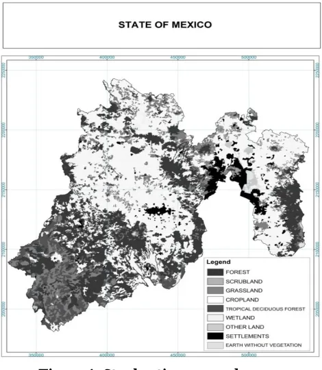
Figure 1: Stochastic approach map
Allometric equations and the factors used to calculate biomass in kilograms per tree and carbon percentage of each species are shown in Table 2:
Table 2: Allometric equations for biomass and factor in calculating carbon by specie
Biomass estimates (B)
(kg/árbol)
Specie coefficient of determination
Carbon conversion factor
0.1033*DN2.39 Quercus sp 0,99 54.00 %
0,0357 * DN2.6916 Pinus patula 0,98 50.31 %
0.0754*DN2.513 Abies religiosa: 0,98 46.48 %
10{-0.535 + 0.966 log 10 (BA)} Dry climate zone (México)
0,94 50.00 %
Table 3: Combined items by specie
Especie Total de puntos
Abies forest 27
Oak forest 60
Oak-Pine forest 29
Pine forest 31
Pine-Oak forest 26
Tropical deciduous forest 22 Bosque bajo abierto 1 Crasicaule scrublands 1
Temperate mountain
forest 2
Tascate forest 2
Savannah 16
Total de puntos 217
Source: Prepared according to the accorded array.
The cluster grouping type for Abiesis shown in Table 4:
Table 4: Cluster of Abies forest
Average value cluster 1 90.36
Average value cluster 2 286.19
Average value cluster 3 504.28
C Ton/ha Point number
ID
NFI Distance Point number
ID
NFI Distance Point number
ID
NFI Distance
1 61616 5 1 61856 69 1 59578 917
2 60320 61 2 59313 69 2 59814 2667
3 60589 443 3 62350 1337 3 59564 3585
4 62362 693 4 62849 1481
5 61592 784 5 62848 1797
6 60603 1035 6 62859 2059
7 59828 1342 7 60605 2358
8 59830 1964 8 62600 3010
9 61855 2167 9 61095 3113
10 60067 3077 10 60859 3254 11 59312 3277 11 62872 3614 12 62850 3359 12 62122 4000
Carbon content per growth phases, are shown in Table 5:
Table 5: Carbon content (ton/ha) assigned to land use by forestry specie
Forestry species
Development of vegetation Secondary
forest without shrub
vegetation
Secondary forest vegetation
Primary forest vegetation
Abies 90.36 286.19 504.28
Quercus 51.49 163.77 294.99
Quercus -Pinus 72.33 178.55 318.10
Pinus 94.11 297.61 543.82
Pinus - Quercus 34.27 125.92 270.39
Tropical
deciduous forest 00.03 000.16 000.44
Source: Based on the carbon content.
Modules CA_Markov and Stchoiceare applied for comparison with current land use mapping (2010) and it is shown in Table 6:
Table 6: Comparison of results (surface in ha)
Clase Stchoice CA_ Markov
Land use 2010
Forest 636947.24 621294.76 625666.24
Scrubland 12938.52 16309.76 14689.56
Grassland 298795.36 316810.84 307351.92
Cropland 1013570.84 1030726.32 1029083.40
Tropical
deciduous forest 119582.48 117338.84 118181.40
Wetland 19903.36 18364.68 18828.80
Other land 19945.36 10168.68 14144.76
Settlements 101121.76 92064.44 94992.20
Earth without
vegetation 10436.28 10217.64 10303.04
Source: Prepared based on the results
Figure 2. Markov chains and cellular automata approach map
The number of isolated cells presented in Figure 1 where diminished considerably upon applying the cellular automata and Markov chain algorithm, this can be seen in Figure 2.To apply this procedure we use the same reference data, i.e. the transition matrixes comparing Series II 2002 and Series III 2002, once projected to 2010 the first one under a random distribution and the former one’s projection includes correlation between first neighbor pixels.
Table 7: Rate of exchange of land use for series III and IV
Categories Series III 2002 (Ha)
Series IV 2010 (Ha)
Rate of exchange Series III and IV
Forest 616933.76 625666.24 0.175
Scrubland 18106.88 14689.56 -2.580
Grassland 327544.28 307351.92 -0.792
Cropland 1033721.72 1029083.40 -0.056
Tropical deciduous forest
117392.32 118181.4 0.083
Wetland 17681.16 18828.80 0.789
Other land 4199.72 14144.76 16.391
Settlements 87576.44 94992.20 1.021
Earth without vegetation
10085.04 10303.04 0.267
Source: Prepared based on the results
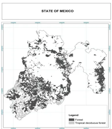
Figure 3: Location of forests and tropical deciduous forest
The content of carbon was calculated per specie, using the established values in Table 5results are shown in Figure 4.
The National Park “Nevado de Toluca”, “Sierra de las Cruces” and “Sierra Nevada” are the zones that present the highest amount of carbon per hectare. While the lowest amount was shown in the tropical deciduous forests located at the south of the state of Mexico. Adding up the content of carbon in all the forest polygons for the state of Mexico shows that the carbon reservoirs for 2010 are 0.167556208 Gt in forests and 13,003 tons in tropical deciduous forests. The before mentioned amount represents 2% of the national reserves, value given be Masera et al. (1997).
4. Discussion
The Intergovermental Climate Change Panel (IPCC, 2006) proposes 6 general categories for Mexico, nevertheless this study for a state level, they where disassemble into 9 categories, differentiating between forests and tropical deciduous forests, between scrubland and grasslands, and finally between other lands and earth without vegetation.
Stchoice module results can be considered as intermediate probabilistic results since it evaluates the markovian transition probabilities between categories of land use in a certain time line. This turns up as a pixel map or isolated dispersed cells that diminish the precision that one would expect for the obtained results.In percentage values, Stchoice module presents higher values, for positive and negative rates, ensuing in a bigger land use change, for example the fraction change in forests is of -1.8, when for CA_Markov module the value would be 0.7; in tropical deciduous forests the values are -1.2 and 0.7 respectively. The average percentage for Stchoice is of -4.6 and 2.4% for CA_Markov, hence the average of the first model underrates and the second overrates.
From their strictly probabilistic function, the transition frequencies between categories, under stable conditions, and taking into account the land cover projections for 2010 lead to a scenario where the hectares of land occupied by forests, tropical deciduous forests, wetlands, other lands, settlements, scrubland, grassland and cropland are overrated and/or underrated.The first resulting scenario, from stochastic analysis draws attention to the recovery of forests and tropical deciduous forests and the second scenario from cellular automata and Markov chains shows the loss of forests and tropical deciduous forests in favor of grassland and cropland surface.
The positive rate of changes presented by forests and tropical deciduous forests, lesser than 0.1% yearly are very small, this can confirm a minimum mending process from small areas of grassland and cropland, hence the vegetation recovery for the following first years and according to the growing stages will give a potential small carbon capture.
This scenario points out the discussion over the increase in a short term, of forest coverage, hence its potential capacity of capturing carbon. The scenario obtained through the applied allometric equations yields focalizing the most important elevations and ratifies the abundance of forest as a main reservoir of carbon in this territory. Its capacity diminishes as the trees aging increases, therefore the importance of taking into account the rate of growth and the intensity of the changes undergoing all year through tree cover in the forest and tropical deciduous forests. This implies a yearlong variation of size, but excludes facts about the delay in the transition from secondary to primary vegetation, knowledge that correlates to the accumulation of biomass.
The existing studies in Mexico about carbon capture are given in a national level or local, the former one by destructive sampling, the presented proposal provides a spatial image of the contents included in the State of Mexico, with and measurable intrinsic error depending on the chosen projection.Any activity that accrues forest coverage implies directly an increase of carbon capture capacity and this is considered as a potential way to mitigate the emissions of CO2 to the atmosphere.
5. Conclusions
In this study, stochastic analysis (Ross, 1996 and Van Kampen, 2003) through Markov chains and the cellular automata integrated spatial analysis and conditional probability description for a local environment, increasing significantly the validation of information from the National Forest Inventory and stochastic projection maps.The cellular automata procedure measured the local contiguity, increasing the possibility of being part of a certain category, integrating a spatial characteristic to the conditional probability, improving considerably the stochastic projection map.This type of model leads to a global and immediate vision for the potential carbon capture by forests, without making localized destructive sampling and avoiding higher investment of time and costs.
The offered model for land use changes is related to changes in carbon reservoirs, which decreases in the central region and remains high in the mountainous areas of the east and southeast of the State of Mexico. Whereas in the tropical deciduous forests, located in the south of the state, less amount of carbon stored.
Acknowledgements
We express our gratitude to Conacyt-Semarnat´s funding under project “Cambios de uso del suelo, inducidos por actividades agropecuarias en ecosistemas terrestres templados y cálidos del Estado de México: Impactos locales y emisiones globales de gases de efecto invernadero”. We acknowledge INEGI for donating six maps of land use Series IV of geology and edaphic under scale 1:250,000. We appreciate Conafor Mexico for granted access to the database of the National Forrestal Inventory corresponding to the State of Mexico. Finally we recognize support received by the Autonomous University of the State of Mexico.
References
Acosta, M., Carrillo, F., Díaz, M. (2009). Determinación del carbono total en bosques mixtos de Pinus patula Schl. Et Cham. TERRA Latinoamericana, 27, 105-114. Avendaño, D., Acosta, M., Carrillo, F., Etchevers, J. (2009). Estimación de biomasa y
carbono en un bosque de Abies religiosa. Fitotecnia Mexicana, 32, 233-238. Comisión Nacional Forestal (CONAFOR). Inventario Nacional Forestal y de suelos
2007-2010. [CD-ROM]. (2011). Guadalajara, México. CONAFOR.
Díaz, R., Acosta, M., Carrillo, F., Buendía, E., Flores, E., Etchevers, J. (2007). Determinación de ecuaciones alométricas para estimar biomasa y carbono en Pinus Patula Schl. Et Cham. Madera y Bosque, 13, 25-34.
Eastman, J.R. (2006). Idrisi Andes. Guide to GIS and Image Processing. Clark Labs, Clark University, USA.
Instituto Nacional de Estadística y Geografía (INEGI). Carta de uso del suelo escala 1:250,000, Serie I. Conjunto Vectorial. [CD-ROM]. (1993). Aguascalientes, México. INEGI.
Instituto Nacional de Estadística y Geografía (INEGI). Carta de uso del suelo escala 1:250,000, Serie II. Conjunto Vectorial. [CD-ROM]. (1997). Aguascalientes, México. INEGI.
Instituto Nacional de Estadística y Geografía (INEGI). Síntesis Geográfica del Estado de México. [CD-ROM]. (2001). Aguascalientes, México. INEGI.
Instituto Nacional de Estadística y Geografía (INEGI). Carta de uso del suelo escala 1:250,000, Serie IV. Conjunto Vectorial. [CD-ROM]. (2010a). Aguascalientes, México. INEGI.
Instituto Nacional de Estadística y Geografía (INEGI). Censo de Población y Vivienda 2010. [CD-ROM]. (2010b). Aguascalientes, México. INEGI.
Intergovernmental Panel Climate Change [IPCC], (2006). Guidelines for National Green
House Inventories. Retrieved from
http://www.ipccnggip.iges.or.jp/public/2006gl/spanish/
Masera, O., Ordoñez.M.J. and Dirzo,R. (1997). Carbon emissions from Mexican forests: current situation and long term scenarios. Climatic Change, 35, 265-295. Masera, O., De Jong, B., Ricalde, I. (2000). Consolidación de la oficina Mexicana de gases de
efecto invernadero, Sector Forestal. Reporte final. Instituto Nacional de Ecología. Ordoñez, J.A. y Masera, O. (2001). Captura de carbono ante el cambio climático.
Madera y bosques. 7, 3-12.
Paegelow, M., Camacho, M. T. y Menor, J. (2003). Cadenas de Markov, evaluación multicriterio y evaluación multiobjetivo para la modelización prospectiva del paisaje, GeoFocus, 3, 22-44.
Palacio, J. L., Bocco, G., Velazquez, A., Mas, J. F., Takaki, F., Victoria, A., … González, F. (2000). La condición actual de los recursos forestales en México: Resultados del inventario forestal nacional 2000.Investigaciones Geográficas, 43, 183-203.
Palacio, J.L., Sánchez, M.T., Casado, J.M., Propin, E., Delgado, J., Velázquez, A., … Camacho,C.G. (2004).Indicadores para la Caracterización y Ordenamiento del Territorio.México, D.F. UNAM, INE, CONANP, CONABIO, INEGI, SEDESOL.
Pimienta, D., Domínguez, G., Aguirrez, O., Hernández, F., Jiménez, J. (2007). Estimación de biomasa y contenido de carbono en Pinus Cooperi Blanco en Pueblo Nuevo, Durango. Madera y Bosque, 13, 35-46.
Ross, S. (1996). Stochastic processes. Ed. John Wiley & Sons, Inc. USA.
Riofrío, G. (2007). Cuantificación del carbono almacenado en sistemas agroforestales en la estación experimental Santa Catalina, INIAP. Licenciatura. Escuela Superior Politécnica de Chimborazo. Riobamba, Ecuador.
SEMARNAT-INE (2006). Inventario Nacional de emisiones de gases de efecto invernadero 1990-2002. México, D.F. Secretaría de Medio Ambiente y Recursos Naturales- Instituto Nacional de Ecología.