Masatoshi YAGI
, ,, Naohiro KASUYA
,, Akihide FUJISAWA
,, Sanae-I. ITOH
,and
Kimitaka ITOH
1,3,6)1)Interdisciplinary Graduate School of Engineering Sciences, Kyushu University, Fukuoka 816-8580, Japan
2)Research Institute for Applied Mechanics, Kyushu University, Fukuoka 816-8580, Japan
3)Itoh Research Center for Plasma Turbulence, Kyushu University, Fukuoka 816-8580, Japan
4)Japan Atomic Energy Agency, Naka, Ibaraki 311-0193, Japan
5)Graduate School of Frontier Sciences, The University of Tokyo, Tokyo 277-8561, Japan
6)National Institute for Fusion Science, Gifu 509-5292, Japan
(Received 5 December 2011/Accepted 27 March 2012)
Preliminary observation results are reported for a new discharge regime in the Plasma Assembly for Nonlin-ear Turbulent Analysis (PANTA), where spontaneous transitions in the equilibrium profile and fluctuation spectra occur. Two different states are defined by using the mean density value. Axial and radial profiles are observed for the two states, and large profile changes are found. The spatiotemporal evolution of the transition front is measured. Changes in the fluctuation spectrum are evaluated using conditional average and lock-in average.
c
2012 The Japan Society of Plasma Science and Nuclear Fusion Research
Keywords: linear plasma, drift wave, turbulence, transition phenomena DOI: 10.1585/pfr.7.2401054
1. Introduction
Plasma turbulence can give rise to intermittent phe-nomena such as spontaneous structure formation or abrupt changes of the fluctuation regime [1]. Fast transitions be-tween quasi-stable turbulent states like the L-H transition [2, 3] have been observed in fusion devices, but their the-oretical understanding remains a challenge [4–6]. Under-standing of such turbulent states and transitions is regarded as an important issue both in physics of non-equilibrium systems and in nuclear fusion research.
Transition phenomena have been successfully studied in several low temperature laboratory plasmas using mul-tipoint measurements of plasma fluctuations [7–9]. In the PANTA, the successor device of the LMD-U, various tur-bulent regimes, some of which feature spontaneous tran-sitions, can be investigated by changing the neutral gas pressure or the magnetic field strength. With a magnetic field strength ofB =0.09 T and high neutral gas pressure
conditions (Pn∼0.40 Pa), a large amplitude coherent fluc-tuation accompanied by higher order harmonics, which is regarded as a drift solitary wave, is seen [10]. When the neutral gas pressure is lowered to an intermediate value (Pn ∼ 0.27 Pa), the PANTA shows a transition region,
author’s e-mail: [email protected]
∗)This article is based on the presentation at the 21st International Toki Conference (ITC21).
where the shape of the fluctuation spectrum switched spon-taneously between two states [8, 9]. Finally, at low neutral gas pressure conditions (Pn ∼ 0.13 Pa), a broad fluctua-tion spectrum is observed that had been associated with a streamer structure in the LMD-U [11, 12]. It has now been discovered, that a transition region can also be observed for a pressure between the intermediate and the low neutral gas pressure condition (atPn∼0.16 Pa). In this regime, transi-tions are observed for the equilibrium profile as well as for the fluctuation spectrum. This article presents preliminary observations in the new transition regime.
2. Experimental Setup
Experimental observations are carried out in the PANTA, a linear cylindrical magnetized helicon plasma. The vacuum vessel of the PANTA has a length of 4050 mm and a diameter of 450 mm. Seventeen linearly aligned magnetic coils generate a homogeneous magnetic field with a fixed magnetic field strength ofB = 0.09 T.
Neu-tral (Argon) gas is fed in a glass tube installed at one side of the device and ionized by a 3 kW, 7 MHz RF source. Neutral gas pressure is monitored with two ion gauges at the source region and two manometers at the central re-gion of the vacuum vessel, and can be controlled with a mass flow controller. The PANTA is equipped with sev-eral Langmuir probes to measure plasma fluctuations. The
c
2012 The Japan Society of Plasma
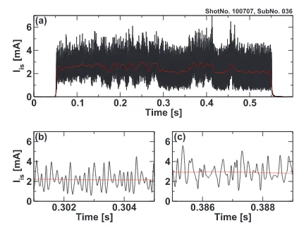
Fig. 1 (a) Typical time evolution of ion saturation current signal measured with one tip of the 64-channel probe array (r=
4 cm,z=1.625 m,θ=0). Red curve shows 0.1 kHz cut-offlow pass filtered signal. Two zoomed time series for the two different states are shown in (b) and (c).
measurement location of each probe tip is given in cylin-drical coordinates, r, θ andz, where the origin of the z
coordinate is defined as the plasma helicon source. In this article, we use three kinds of probe sets: a 64-channel az-imuthal probe array (r=4 cm,z=1.875 m,−π < θ < π),
a 5-channel radial probe array (2<r<6 cm,z=1.625 m, θ =π), and a 4-point axially aligned probe set (r=4 cm,
z = 1.125,1.625,1.875 and 2.625 m, θ = 0) to observe the three-dimensional evolution of the transition front and fluctuation. We use one tip of the 64-channel azimuthal probe array atθ=0 as a reference to detect the onset of the transition. The ion saturation current fluctuations are mea-sured with a temporal resolution ofΔt =1µs, and can be used as an index of the electron density fluctuations [13].
3. Experimental Results
3.1
Identification of the transition
Figure 1 shows the typical time evolution of the ion saturation current signal measured with the reference probe. The red dashed curve shows the low pass filtered signal using a cut-offfrequencyfc=0.1 kHz. The low pass filtered signalIis0 follows the mean density evolution dur-ing the discharge. It is easy to see thatIis0transits between a lower and higher value. Time series for each state can be selected manually and examples are given in Fig. 1 (b) for the lower mean density and Fig. 1 (c) for the higher mean density. Qualitative differences in the fluctuations’ shape are seen. To discuss the changes inIis0more quantitatively and detect transitions automatically, we first inspect the normalized histogram of the Iis0 value which is given in Fig. 2 for 50 discharges. Two separate peaks appear in the normalized histogram and are the sign of a bifurcation in
Iis0between two different states. We assume the probabil-ity densprobabil-ity ofIis0for each state has the shape of a Gaussian distribution. The nonlinear least squares Gaussian fitting for each peak are shown by red and green curves in Fig. 2,
Fig. 2 Normalized histogram ofIis0. The two fitting curves (red and green) are Gaussian fits for the two peaks. Labels show mean value and standard deviation of the fitted Gaussians.
where the mean values and standard deviations for each Gaussian are indicated in the labels. Using these Gaussian parameters, we can explicitly define two states, called the lower and upper state, as|Iis0−μ1| ≤σ1and|Iis0−μ2| ≤σ2, respectively. Because the area in the normalized histogram for the lower state is much larger than the one for the upper state, the plasma is predominantly in the lower state, and sometimes abruptly transits to the upper state. We define the transition onset time as the moment in time when the
Iis0signal rises to the threshold valueμ2−σ2(we call a fall below the threshold value an inverse transition).
3.2
Changes in the equilibrium profiles
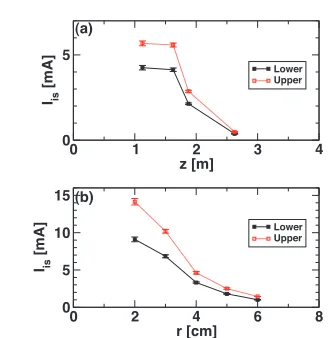
Figures 3 (a) and (b) show axial and radial profiles for the two states calculated with conditional averaging. Typical transition time is a few milliseconds. In the axial profile, values of averagedIis decay as the axial positionzincreases in both states, presumably due to plasma re-combination loss. However, characteristicIis fluctuations at different axial positions are qualitatively similar and their cross coherences are quite high for specific modes. We may therefore regard the plasma turbulence as two-dimensional even if a density gradient exists in the axial direction. Differences inIis0 profiles are seen in both the axial and radial direction for the two states. In the plasma core region, atr=2 cm,Iischanges by 30-40%.
We estimate the spatiotemporal evolution of equilib-rium profiles transition in both axial and radial direction using the low pass filtered signals. Cross Correlation Func-tion (C.C.F) is calculated between the signals at two dif-ferent axial (radial) positions for over 90 transitions and inverse transitions, and we obtain time lagsτwith quite high C.C.F values. Figure 4 is a plot of the time lagτ as a function of measurement location. In the axial di-rection, shown in Fig. 4 (a), the time lag is computed by using the probe tip atz = 1.125 m, closest to the source
Fig. 3 Conditional averaged (a) axial and (b) radial profiles for the upper and lower states. Error bars show the standard deviation from over 90 distinct transitions in 50 shots.
Fig. 4 Time lags of transition and inverse transition onsets in the (a) axial and (b) radial direction, calculated with ref-erence probes atz=1.125 m andr=2 cm, respectively.
delay for the plasma near the source regionz<1.125 m is
quite small, showing that the transition occurs simultane-ously in this region. Roughly estimated propagation speed atz∼1−2 m is slightly less than∼2000 m/s, which is of the order of the ion sound speedCs∼2000 m/s. Far from the source region, atz > 2 m, a decrease in the electron temperature is expected, resulting in a decrease ofCs. This could be linked with the observed propagation speed de-cay, but more data is necessary to confirm this observation, as error bars are too large in Fig. 4 to conclude unambigu-ously. In the radial direction, the valueτis calculated with respect to a reference atr=2 cm and is shown in Fig. 4 (b). Negativeτdecreasing with increasingris observed. The transition seems to first occur at the edge region and to de-velop towards the core region with a characteristic speed of ∼60 m/s. Again, time lag in the core region ofr<2 cm is quite small. In general, the propagation speed can be quite different for each transition event, resulting in large error bars that make statistical quantitative evaluation difficult.
propagation of the ion saturation current fluctuations is ob-served with every other tip of the 64-channel probe array. We define the positive direction for the azimuthal angleθ as the direction of electron diamagnetic drift. Windowed Fourier Transform (FT) is performed for both time and azimuthal space to calculate the two-dimensional power spectral density as a function of frequency f and az-imuthal mode numberm, where the sign of the mode num-ber gives the propagation direction. A time window of
ΔT = 3 ms is used to obtain a frequency resolution of
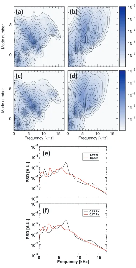
Δf =0.3 kHz. Figures 5 (a) and (b) are conditional
aver-aged power spectral density for the lower and upper states. In the lower state, the dominant fluctuating mode is located at (m,f)=(2,6.7 kHz). In addition, a counter-propagating mode at (m,f)=(−1,1.3 kHz) is excited. In the upper state, the counter-propagating mode is still observed but its frequency slightly changes to f =1.0 kHz. The mode
number and frequency of the dominant mode are changed to (m,f)=(1,2.3 kHz). The broad spectra can have many combinations of wave coupling. In particular, three-wave couplings involving the counter-propagating mode have been considered playing an important role for the nonlinear excitation process of the streamer structure in the LMD-U [12]. We discuss similarities between the spectra for the two states and the spectra obtained for discharges with slightly decreased and increased neutral gas pressure. In both neighboring neutral gas pressure conditions, no transitions are observed, and fluctuation spectra remain un-changed during the whole discharged. Fluctuation spectra for the cases ofPn =0.13 Pa andPn =0.17 Pa are drawn in Figs. 5 (c) and (d). To see differences in the spectra more quantitatively, mode number integrated power spec-trum densities for Figs. 5 (a) and (b), and Figs. 5 (c) and (d) are shown in Figs. 5 (e) and (f), respectively. The fluctua-tion spectrum in the lower state is similar to the one in the
Pn =0.13 Pa case, and the spectrum in the upper state re-sembles the one in thePn =0.17 Pa case. Assuming that the two pairs of similar spectra indicate same fluctuation states, there might be possible multiple fluctuation states at this regime.
In the last part of the present article, we observe the time evolution of fluctuating mode power during the tran-sition and inverse trantran-sition using the lock-in average tech-nique. The lock-in average at the moment of the transition and inverse transition is defined as ¯x(τ)=1/NNi=1x(ti+
τ), where τ = −MΔt/2,−(M −1)Δt/2, . . . ,0, . . . ,(M −
Fig. 5 Conditional averaged two-dimensional power spectral density for (a) the lower state and (b) the upper state. For comparison, the spectra for discharges in the (c)
Pn =0.13 Pa case and (d)Pn =0.17 Pa case are shown. Mode number integrated power spectrum density of (a) and (b) is shown in (e) and that of (c) and (d) is shown in (f).
indicates the i-th transition (or inverse transition) andN
is the total number of transitions (or inverse transitions). It should be noted that this lock-in average is generally called conditional average and is widely used (e.g., to ob-serve shapes of plasma blobs [14]). Here, we focus on two characteristic modes in the lower state, i.e., the modes at (m,f)=(2,6.7 kHz) and (m,f)=(−1,1.3 kHz). The time window of the FT is shifted by steps of 0.05 ms to ob-tain the time evolution of the spectrum. The power spec-tral density of them = 2 mode is integrated over a fre-quency range corresponding to the half-width of the mode. For the counter-propagating mode, we use the integration
Fig. 6 Time evolution of (a) and (b)Iis0signal, (c) and (d) fluc-tuating mode powers of the counter-propagating mode, and (e) and (f) those of them=2 mode, calculated using lock-in average for transitions and inverse transitions.
range 0 kHz≤ f ≤ 3.0 kHz to account for the slight
fre-quency change during the transition. Figures 6 (a), (c) and (e) show the lock-in averaged time series ofIis0 and fluc-tuation powers for the counter-propagating mode and the
m = 2 mode, around the moment of the transition. Fig-ures 6 (b), (d) and (f) are the corresponding plots for the inverse transition. The error bars represent standard devia-tion. One can compare the time series of the mode power variation with that ofIis0. For the transition case, first the power of the counter-propagating mode starts to increase, that of them=2 mode starts to decrease and theIis0starts to increase. After a few millisecond, the evolution of the counter-propagating mode changes and its power starts to decrease. For the inverse transition, growth of the counter-propagating mode power and accompanying decrease of
Iis0 is seen before the growth of them = 2 mode power. Moments with strongm = 2 mode power seem to be re-lated to a damping of the counter-propagating mode power in both cases. This may imply that an energy interchange exists between these two modes. As shown in Fig. 6, the causal relation between fluctuation power variation and
Iis0 variation is not easy to clarify. Indeed, an interac-tive connection exists between fluctuations and mean den-sity. Changes in fluctuations can vary the profile through changes in transport, and changes in the profile can also affect fluctuations by changing the growth rate of the fluc-tuations. To draw a conclusion, further measurements are needed to study the dynamics of the transport and gradi-ents.
4. Summary
region, and to evolve towards the end plate. A charac-teristic speed close toCs was estimated in the middle of the plasma column. In the radial direction, the transition seemed to start close to the edge of the plasma and to de-velop towards the core region at a speed of∼60 m/s.
Two-dimensional Fourier power spectral density was calculated as a function of frequency and azimuthal mode number. Conditional averaged power spectra in the two different states were found to be similar to the averaged power spectra at both neighboring neutral gas pressure conditions, implying that there might be multiple fluctu-ation states for the transition conditions. In the last part of this article, we showed lock-in averaged time sequences of fluctuating power for several characteristic modes dur-ing the transition and inverse transition. Possible evidence could be presented that energy was exchanged between several modes.
[2] F. Wagneret al., Phys. Rev. Lett.49, 1408 (1982). [3] M. Nagamiet al., Nucl. Fusion24, 183 (1984). [4] S.-I. Itohet al., Phys. Rev. Lett.60, 2276 (1988). [5] P. Diamondet al., Phys. Rev. Lett.72, 2565 (1994). [6] J. Cordeyet al., Nucl. Fusion35, 101 (1995).
[7] Y. Nagashimaet al., J. Plasma Fusion Res. SERIES8, 50 (2009).
[8] H. Arakawaet al., Plasma Phys. Control. Fusion51, 85001 (2009).
[9] H. Arakawa et al., Plasma Phys. Control. Fusion 52, 105009 (2010).
[10] H. Arakawa et al., Plasma Phys. Control. Fusion 53, 115009 (2011).
[11] T. Yamadaet al., Nat. Phys.4, 721 (2008).
[12] T. Yamadaet al., Phys. Rev. Lett.105, 225002 (2010). [13] K. Kawashima et al., Plasma Fusion Res. 6, 2406118
(2011).