GENERATION OF DNA STRUCTURES
by
Michael D. Tobiason
A dissertation
submitted in partial fulfillment of the requirements for the degree of
Doctor of Philosophy in Material Science and Engineering Boise State University
DEFENSE COMMITTEE AND FINAL READING APPROVALS
of the dissertation submitted by
Michael D. Tobiason
Dissertation Title: In Silico Sequence Optimization for the Reproducible Generation of DNA Structures
Date of Final Oral Examination: 15 October 2019
The following individuals read and discussed the dissertation submitted by student Michael D. Tobiason, and they evaluated the student’s presentation and response to questions during the final oral examination. They found that the student passed the final oral examination.
William L. Hughes, Ph.D. Chair, Supervisory Committee Bernard Yurke, Ph.D. Member, Supervisory Committee Jeunghoon Lee, Ph.D. Member, Supervisory Committee James Alexander Liddle, Ph.D. Member, Supervisory Committee Igor L. Medintz, Ph.D. Member, Supervisory Committee
iv DEDICATION
v
ACKNOWLEDGMENTS
Thank you first and foremost to my dissertation committee for the time and effort they have spent shaping this project: Dr Hughes, Dr. Yurke, Dr. Lee, Dr. Liddle, and Dr. Medintz. Your feedback has been fundamental to improving both the science and my approach to the science. Special thanks to Bernie for sitting down with me in September 2014 and teaching me to code in Java. I never expected that the relatively simple program we created would evolve into this PhD dissertation. Another special thank you to Will for his limitless patience with me over the years. I have learned more from you than I will ever be able to explain or put into words.
Thank you to all the faculty and staff at Boise State who I have had the pleasure to work with. Special thanks to Natalya Hallstrom, Elton Graugnard, Jennifer Padilla, Reza Zadegen, Wan Kuang, Bill Knowlton, Paul Davis, and Donald Kellis.
vi ABSTRACT
Biologically, deoxyribonucleic acid (DNA) molecules have been used for information storage for more than 3 billion years.1 Today, modern synthesis tools have made it possible to use synthetic DNA molecules as a material for engineering nanoscale structures. These self-assembling structures are capable of both resolutions as fine as 4 angstroms and executing programed dynamic behavior.2,3 Numerous approaches for creating structures from DNA have been proposed and validated, however it remains commonplace for engineered systems to exhibit unexpected behaviors such as low formation yields, poor performance, or total failure. It is plausible that at least some of these behaviors arise due to the formation of non-target structures, but how to quantify and avoid these interfering structures remains a critical question.
vii
viii
TABLE OF CONTENTS
DEDICATION ... iv
ACKNOWLEDGMENTS ... v
ABSTRACT ... vi
LIST OF TABLES ... xi
LIST OF FIGURES ... xiii
LIST OF ABBREVIATIONS ...xviii
CHAPTER ONE: INTRODUCTION ... 1
Section 1.1 – Motivation ... 1
Section 1.2 – The Structure of a DNA Molecule ... 3
Section 1.3 – The B-DNA Structure ... 4
Section 1.4 – Creating Shapes and Assemblies Using B-DNA ... 5
Section 1.5 – State of the Art Design Procedures ... 7
Section 1.6 – Non-Target Structures ... 8
Section 1.7 – Defining Structural and Dynamic Behavior ... 9
Section 1.8 – Sequence Symmetry Minimization ... 10
Section 1.9 – Improving the State-of-the-Art ... 12
CHAPTER TWO: QUANTIFYING SEQUENCE FITNESS ... 16
Section 2.1 – Quantifying Variations in Dynamic Behavior ... 16
ix
Section 2.3 – Do B-DNA Structures Explain Kinetic Variation? ... 21
Method and Results ... 22
Discussion ... 26
Section 2.4 – Are TFS-Fit Sequences Kinetically Uniform? ... 27
Methods and Results ... 27
Discussion ... 41
Section 2.5 – Further Discussion ... 48
Section 2.6 – Conclusions ... 50
CHAPTER THREE: AN ALGORITHM FOR GENERATING FIT SETS OF DNA OLIGONUCLEOTIDES ... 52
Section 3.1 – The Remarkable Number of Potential Systems ... 52
Section 3.2 – An Evolutionary Heuristic Algorithm ... 53
Section 3.3 – Is the Algorithm Efficient Enough? ... 58
Method and Results ... 58
Discussion ... 64
Section 3.4 – How Effective is the Algorithm Compared to Other Software? ... 65
Methods and Results ... 65
Discussion ... 67
Section 3.5 Conclusions ... 67
CHAPTER FOUR: SOFTWARE IMPLEMENTATION STRATEGIES ... 69
Section 4.1 – Software Architecture Briefly Explained ... 69
Section 4.2 – Strategies for Improving Software Efficiency ... 70
Efficiently Scoring Systems ... 70
x
Section 4.4 – Can the Software Improve Published Systems? ... 74
Methods and Results ... 75
Discussion ... 79
Section 4.4 Conclusions ... 80
CHAPTER FIVE: ENGINEERING SYSTEMS WITH UNIFORM BEHAVIOR ... 81
Section 5.1 – Key Findings ... 81
Section 5.2 – The method ... 83
Section 5.3 – Conclusions and Future Work ... 84
APPENDIX A ... 86
APPENDIX B ... 259
xi
LIST OF TABLES
Table 2-1 Select properties of the fittest systems in each criterion/dataset
combination. Reported values include: the duplex-formation rate kDF, the median rate (M), the Median-Absolute-Deviation of rates (MAD), and P-values calculated using a two-sample Kolmogorov-Smirnov test. ... 25 Table 2-2 Arrhenius parameters extracted from the duplex-formation rates (kDF) of
each implementation. The activation energy (Ea), pre-exponential factor (A), and R2 of the Arrhenius fit are reported. ... 38 Table 3-1 Parameter values for each parameter-set used in the “Global” sampling of
algorithm efficiencies. ... 60 Table 3-2 Typical non-target structures present in 35 bp duplexes generated using
several publicly-available software tools. ... 66 Table 4-1 Select properties from the four re-engineered systems. ... 79 Table A.1 New sequences for the model system presented in Figure 2-5. The
nomenculture for strand names is consistent with the disseration text. .... 87 Table A.2 System, temperature, and experiment number for the 82 sets of
fluorescence measurements. Each experiment consisted of up to three samples, including a dye only control, duplex formation reaction, and strand displacement reaction. Experiments 32-37 and 39-44 were used to study the reproducibility of the measurement process, and contain only the duplex-formation reaction or the strand-displacement reaction as a
consequence. ... 90 Table B.1 New sequences for the 10x10x10 DNA brick reported by Ke et al.30 .... 260 Table B.2 Non-target structures present in the sequences for the 10x10x10
DNA-brick structure.30 ... 273
Table B.3 New sequences for the “Four-Input OR gate” seesaw-gate based system published by Qian et al.29 ... 274 Table B.4 Non-target structures present in the “Four-Input OR” seesaw-gate based
xii
Table B.5 New sequences for the autocatalytic-four-arm-junction system published by Kotani et al.65... 277
Table B.6 Non-target structures in the autocatalytic-four-arm-junction system
published by Kotani et al. ... 278 Table B.7 New sequences for the autocatalytic system published by Zhang et al.25
... 280 Table B.8 Non-target structures in the autocatalytic system published by Zhang et
xiii
LIST OF FIGURES
Figure 1-1 The Boise State logo self-assembled using synthetic DNA strands. (left) Atomic force microscopy image showing numerous structures. (right) Isolated and processed image of a single structure. Structure design by Kelly Schutt. Images captured and processed by Brett Ward and Elton Graugnard. ...2 Figure 1-2 Chemical structure of DNA molecules. (Left) Chemical structure of the
four sub-structures of which DNA molecules are composed: deoxyribose, phosphoric acid, and the four nucleobases. (Right) Chemical structure of an example DNA molecule containing the sequence 5’-GCAT-3’. Images adapted from the atdbio website (www.atdbio.com)...4 Figure 1-3 Three illustrations of B-DNA structures. (a) Chemical structure of two
complementary DNA 4-mers. (b) A cartoon depicting two interacting DNA 16-mers in the double-helical B-DNA structure. (c) An atomic representation of a 17 base-pair B-DNA structure. Each schematic is adapted from Molecular Biology of the Gene by J. D. Watson.16 ...5
Figure 1-4 Typical state-of-the-art design process illustrated using the DNA Bricks architecture. (a) In the DNA-Bricks architecture target structures are rendered on an abstract 3D canvas where B-DNA duplexes are represented by cubic voxels. (b) DNA strands with sequences implementing the target structure are generated. (c) Strands are chemically synthesized, assembled into the target structure, and are experimentally characterized (TEM Image). (d) Diagram illustrating three key steps in the design process. Images a-c adapted from Ke et al.30 ...7 Figure 1-5 A simple model system described at three levels of decreasing abstraction.
(a) Strand-level abstraction. (b) Domain-level abstraction. (c) Sequence-level abstraction. ...8 Figure 1-6 B-DNA type structures which the simple model system may form. (a) The example system is composed of two strands named Strand-1 and Strand-2. (b) The list of all unrelated or “unique” intermolecular B-DNA type structures this system may form. (c) The list of all intramolecular B-DNA type structures this system may form. ...9 Figure 1-7 Visual summary of the proposed process for generating DNA systems.
xiv
Sequence-Evolver (abbreviated SeqEvo) software for generating in silico optimized sequences, and the Device Profiler (abbreviated DevPro) software for generating detailed reports characterizing existing systems. 14 Figure 1-8 Key aspects of this dissertation and their interrelationships. (top) Three
new optimization criteria were developed. (left) Two new software tools were created. (right) A new sequence generation algorithm was developed. (center) The optimization criteria, heuristic algorithm, and software tools were used to generate samples for experimental characterization. ... 15 Figure 2-1 (a) Flow chart of typical design process with feedback from experimental
characterization to implementation process highlighted. (b) Hata et al. studied the formation rates of 47 implementations of a 23-bp duplex at a temperature of 25°C.37 (c) Zhang et al. studied the formation rates of 99 implementations of a 36 base-pair duplex at temperatures of 37°C and 55°C.36 (d) Reaction rates reported in the three data sets presented as points and summarized by a median line, a box connecting the 25th and 75th percentiles, and bars connecting the min and max values. ... 18
Figure 2-2 Calculation of Network Fitness Score (NFS), Strand Fitness Score (SFS), and Total Fitness Score (TFS). (a) Sequences from the model system presented in Figures 1-5. (b,c) Structural profiles summarizing the “complete” sets of intermolecular and intramolecular structures. (d,e) Calculation of NFS, SFS. (f) TFS is calculated as a weighted linear combination of SFS and NFS. By manipulating the C1 and C2 weights,
TFS can be tuned to emphasize either NFS or SFS. ... 21 Figure 2-3 Effectiveness of different fitness criteria at identifying kinetically uniform
sequences. (a) Cartoon of the criterion evaluation method. (b)
Hybridization rates of the fittest systems within each dataset, as judged by one of the four criteria. Three datasets were analyzed: measurements by Hata et al.37 at 25°C (H25), measurements by Zhang et al.36 at 37°C (Z37), and measurements by Zhang et al.36 at 55°C (Z55). (c) P-values
calculated by comparing the fittest systems to the associated general population (labeled “none”). ... 23 Figure 2-4 Tuning of the Total Fitness Score (TFS) weighting parameters to achieve
statistically significant P-values. Three datasets were analyzed: measurements by Hata et al.37 at 25°C (H25, orange squares), measurements by Zhang et al.36 at 37°C (Z37, green circles), and measurements by Zhang et al.36 at 55°C (Z55, blue triangles). P-values
xv
Figure 2-5 A model system for studying the impact of non-target structures on reaction kinetics. (a) Three strands compose the model system. (b) The two target structures in the model system. (c) Schematic of the duplex-formation target reaction. (d) Schematic of the strand-displacement target reaction... 28 Figure 2-6 Variable sequences for the twelve systems generated to implement the
model system design presented in Figure 2-5. A full list of strand
sequences is provided in appendix A.1... 30 Figure 2-7 Structural profiles of the twelve generated systems. (a) Intermolecular
(left) and intramolecular (right) profiles of the three randomly generated systems. (b) Profiles of the three TFS-fit sequences. (c) Profiles of the three SFS-fit sequences. (d) Profiles of the three NFS-fit sequences. These structural profiles are complete in the sense that they contain all non-target structures, including those which exist within a larger structure. ... 31 Figure 2-8 Method for experimentally characterizing reaction kinetics. (a) One of the generated systems for use as an example. (b) Dye/quencher functionalized strands were prepared at pre-determined experimental conditions. (c) Sample fluorescence was monitored in real-time. (d) Plot of inverse strand concentration vs elapsed time. (e,f) Linear fits applied to all data
preceding reaction half completion in d. ... 33 Figure 2-9 Experimentally determined duplex-formation (kDF) rates for the twelve
implementations of the model system. The discrete data points are connected by lines to aid the eye. Experiments were performed in
triplicate for the TFS-3 system at 20 °C and 40 °C. The error bars on these data points span from the mean to the standard deviation of the three measurements. ... 36 Figure 2-10 Arrhenius fits to the experimentally determined duplex-formation (kDF)
rates for the twelve implementations of the model system. Discrete data points are shown as symbols, with lines illustrating a linear fit to the data. ... 37 Figure 2-11 Experimentally determined strand-displacement rates for the twelve
implementations of the model system. Experiments were performed in triplicate for the TFS-3 system at 20 °C and 40 °C. The error bars on these data points span from the mean to the standard deviation of the three measurements. ... 40 Figure 2-12 Observed correlation between the natural log of the Arrhenius
xvi
Figure 2-13 Experimentally determined duplex-formation rates (symbols) modeled using the empirically derived kinetic model reported in the text (dashed lines). ... 45 Figure 2-14 Kinetic reproducibility of the TFS-optimized implementations compared
to the unoptimized RND implementations. (a) M/MAD ratios calculated from the duplex formation (kDF) rates. (b) M/MAD ratios calculated from
the strand displacement (kSD) rates. ... 48
Figure 3-1 Pseudocode and key parameters describing the evolutionary algorithm. (a) High-level pseudocode illustrating the structure of the nested for loops and the naming conventions. (b) Parameters controlling the structure of the search. All parameters are given a positive integer value at runtime. (c) More detailed pseudocode further illustrating the search process. ... 55 Figure 3-2 The algorithm utilizes a clone-then-mutate approach to generate new
sequences. (a) Diagram illustrating the process for mutating a system’s sequences. (b) The three types of mutations. (c) Diagram illustrating how valid/invalid systems are identified. ... 56 Figure 3-3 Example shape of the search for fit systems resulting from algorithm
execution. (a) Example values for the five key parameters controlling the algorithm: Number-of-Lineages (NL), Cycles-Per-Lineage (CPL),
Number-of-Mothers-Per-Cylce (NMPC), Number-of-Daughters-Per-Cycle (NDPC), and Generations-Per-Cycle (GPC). (b) Visual depiction of search progression for the example parameter values. Sequence
uniqueness (horizontal axis) as a function of time (vertical axis, increasing downward). ... 57 Figure 3-4 Efficiencies measured for varying parameter-sets. (a) The global search
for efficient parameter sets. Efficiencies were measured for 31 parameter-sets spanning parameter space. For each parameter-set 81 independent design trials were conducted, and the efficiency was calculated for each. The observed efficiencies are summarized using a median line, box connecting the 25th and 75th percentiles, and bars connecting the min and max values. (b) The local search for efficient parameters. Parameter-set 5 (orange box) was identified as a highly efficient region in parameter-space. This region was investigated in greater detail by systematically varying each parameter while monitoring efficiency. For each new
xvii
Figure 4-1 Illustration of how the scoring module calculates the strand alignments for a given system. Only the alignments for the Strand 1/Strand 1 combination are shown. ... 71 Figure 4-2 Illustration of how the scoring module calculates fitness scores for each
strand alignment. ... 73 Figure 4-3 (a) Illustration of an example search structure. (b) The number of device
objects which are kept in memory for the given search structure. ... 74 Figure 4-4 Profile of non-target structures in the 10x10x10 DNA-brick before (grey)
and after (blue) sequence optimization.30 ... 77 Figure 4-5 Profile of non-target structures in the “four-input or” seesaw-gate system
before (grey) and after (blue) sequence optimization.29 ... 77 Figure 4-6 Profile of non-target structures in the autocatalytic four-arm junction
system before (grey) and after (blue) sequence optimization.65 ... 78 Figure 4-7 (a) Intramolecular and (b) intermolecular profiles of non-target structures
in the autocatalytic system published by Zhang et al. before (grey) and after (blue) sequence optimization.25 ... 78 Figure 5-1 Key elements of this dissertation. (a) The five studies supporting creation
of the design method. (b) Venn diagram illustrating the interconnected nature of the criteria, algorithm, and software. Studies have been generally associated with key areas to demonstrate their relative contributions to the dissertation. ... 82 Figure 5-2 A process for creating kinetically uniform DNA devices utilizing in silico
xviii
LIST OF ABBREVIATIONS
3’- The 3’ end of a DNA molecule’s phosphate chain
3D Three Dimensional
5’- The 5’ end of a DNA molecule’s phosphate chain
A Adenosine
Approx. Approximately
AFM Atomic Force Microscopy
B-DNA Double helical structure adopted by two complementary DNA strands. B is a historical reference to the name of the second of Franklin and Gosling’s X-ray powder photographs.
bp Base Pair
BHQ2 Black Hole Quencher 2. A proprietary dye-quenching molecule
BSU Boise State University
C Cytosine
CPL Cycles-Per-Lineage
DevPro Device Profiler (custom written software) DNA Deoxyribonucleic acid (class of biomolecules)
eq. Equation
e.g. Latin “exempli gratia” (literally meaning “for example”) et al. Latin “et alia” (literally meaning “and others”)
G Guanine
GPC Generations-Per-Cycle
xix
ml milliliter
NFS Network Fitness Score
NDPM Number-of-Daughters-Per-Mother
NL Number-of-Lineages
NMPC Number-of-Mothers-Per-Cycle
nM nano-Molar
nm nanometer
№ Number of
SeqEvo Sequence Evolver (custom written software) SFS Strand Fitness Score
SS Sequence Symmetry (property for describing system quality) SSM Sequence Symmetry Minimization (sequence optimization
method)
T Thymine
CHAPTER ONE: INTRODUCTION Section 1.1 – Motivation
The allure of self-assembly has long fascinated scientists. To understand why, one needs to look no further than a mirror. Each adult human starts as little more than a single cell. This cell begins a replication cascade leading to approximately 30 trillion cells and a host of interconnected non-cellular structures.4,5 These structures have feature sizes ranging from Angstroms (e.g. chemicals such as DNA) to meters (e.g. extremities such as legs) and are produced with remarkable precision. In a sense, we do not create new humans; we instead create a single cell, which then autonomously fabricates a new human. In today’s terms this may be called a bottom-up self-assembly process. As such, we exist as a proof-by-example that systems of incredible complexity can be created using such techniques. In comparison, state-of-the-art synthetic self-assembled structures remain somewhat trivial. However, even the relatively simple structures already
achievable are showing potential to revolutionize society in applications such as medical diagnostics and information storage.6-12
DNA. In biological self-assembly, the information stored in DNA directs the assembly of structures form a variety of larger materials. As such, it is unlikely that systems created solely from DNA will ever rival the complexity of biological systems. However, advancements in our ability to understand and control DNA structures may yield both technological advancements in the near term and remarkable technologies in the long term.
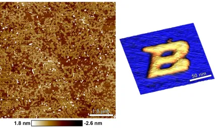
Figure 1-1 The Boise State logo self-assembled using synthetic DNA strands. (left) Atomic force microscopy image showing numerous structures. (right) Isolated and processed image of a single structure. Structure design by Kelly Schutt. Images
captured and processed by Brett Ward and Elton Graugnard.
This dissertation will detail an important advancement toward these goals. I will begin by explaining the basics of DNA structures, and how these have been used to create self-assembling shapes. Next, I will present three criteria we have developed for
structures. Finally, I will explain how we combined our criteria and algorithm to create a software package for automating the design process. I will conclude by discussing the context of these projects, and how I anticipate they may impact the scientific community.
Section 1.2 – The Structure of a DNA Molecule
Chemically, DNA molecules are composed of six sub-structures: deoxyribose, phosphoric acid, and four nucleobases (Figure 1-2, Left). The four nucleobases are Adenine, Cytosine, Guanine, and Thymine (abbreviated A, C, G, and T, respectively). A deoxyribose can be covalently bonded both with phosphoric acid and one of the four nucleobases to create a structure termed a nucleotide. The resulting structure has two exposed OH groups which are referred to as the 5’ site (attached to the phosphorus) and the 3’ site (part of the deoxyribose). Nucleotides are linked by the covalent bonding of one nucleotide’s 5’ site with the 3’ site of the other. This enables the creation of linear chains of polynucleotides which are commonly known as DNA molecules or DNA strands (Figure 1-2, right). Consequently, the chemical structure of a given DNA strand can be fully described by listing the sequence of its bases starting from the 5’ or 3’ end of the structure (for example, 5’-GCAT-3’ in Figure 1-2 right). This structural motif implies that for DNA molecules containing L bases, there are 4L possible base sequences. For
Figure 1-2 Chemical structure of DNA molecules. (Left) Chemical structure of the four sub-structures of which DNA molecules are composed: deoxyribose,
phosphoric acid, and the four nucleobases. (Right) Chemical structure of an example DNA molecule containing the sequence 5’-GCAT-3’. Images adapted from
the atdbio website (www.atdbio.com).
Section 1.3 – The B-DNA Structure
Circa 1953 it was recognized that certain DNA sequences adopt structures now known formally as B-DNA and colloquially as the DNA double-helix.13,14 The B-DNA structure arises from the pairing of complementary bases (A with T or C with G)
arranged on oppositely-oriented phosphate backbones (e.g. 5’-ACTG-3’ and 5’-CAGT-3’ in Figure 1-3a). The binding of a single complementary base is relatively unstable, but structural stability increases for stretches of complementary bases. Such stretches of complementary bases are commonly referred to as either domains or simply
Figure 1-3 Three illustrations of B-DNA structures. (a) Chemical structure of two complementary DNA 4-mers. (b) A cartoon depicting two interacting DNA
16-mers in the double-helical B-DNA structure. (c) An atomic representation of a 17 base-pair B-DNA structure. Each schematic is adapted from Molecular Biology of
the Gene by J. D. Watson.16
Spatially, B-DNA structures adopt the iconic double-helical shape which is emblematic of DNA (Figure 1-3b,c). This structure has a diameter of approximately 2 nm when hydrated and a righthanded orientation. B-DNA has a repeat unit of ~10.5 base-pairs per helical turn and includes both major and minor grooves (Figure 1-3c). These grooves are approximately 2.2 nm and 1.2 nm in width respectively. DNA molecules have been demonstrated to form a host of other structures including triplex and
quadruplex structures; however B-DNA is expected to be the dominant structure under typical experimental conditions.17 In fact, certain DNA structures form via the same complementary sequences however are not B-DNA. Therefore, when discussing complementary DNA sequences, it is more appropriate to describe their propensity to form B-DNA type structures instead of specifically B-DNA itself.
Section 1.4 – Creating Shapes and Assemblies Using B-DNA
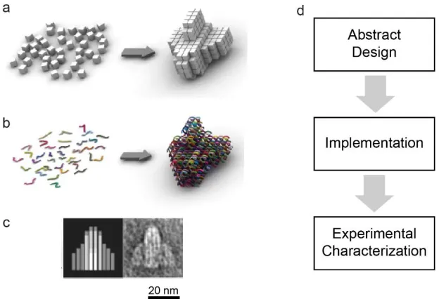
Based on the specificity of B-DNA binding it is possible to rationally design sets of DNA strands – referred to here as DNA systems – which form target structures. Many
b c
Figure 1-4 Typical state-of-the-art design process illustrated using the DNA Bricks architecture. (a) In the DNA-Bricks architecture target structures are rendered on an abstract 3D canvas where B-DNA duplexes are represented by cubic
voxels. (b) DNA strands with sequences implementing the target structure are generated. (c) Strands are chemically synthesized, assembled into the target structure, and are experimentally characterized (TEM Image). (d) Diagram illustrating three key steps in the design process. Images a-c adapted from Ke et al.30
Section 1.5 – State of the Art Design Procedures
Most state-of-the-art design methods follow a workflow similar to that of DNA-bricks (Figure 1-4d). First, target structures are architected using some level of
Section 1.6 – Non-Target Structures
To better understand the issue of non-target structures and the importance of sequence optimization, consider the model system presented in Figure 1-5 below. First, the goal of the system is established as creating two strands which will form a single B-DNA structure (Figure 1-5a). Towards this goal, we can create a domain-level design such as that in Figure 1-5b. In this design, one strand is composed of the alpha domain and the other the complement of the alpha domain (underlined alpha). This design can then be implemented by assigning specific sequences to the alpha domain such as those in Figure 1-5c. For the example implementation, we have chosen the six-base sequence 5-AATTCG-3 for alpha and this implies the sequences for the remainder of the system. As such, this system is one of 46 = 4,096 possible sequence-sets implementing the design.
Figure 1-5 A simple model system described at three levels of decreasing abstraction. (a) Strand-level abstraction. (b) Domain-level abstraction. (c)
Sequence-level abstraction.
discarding any structure which exists as part of a larger structure, the list of all unrelated or “unique” B-DNA structures can be reported (Figure 1-6b). For this example, we see that there are five total intermolecular structures which are unique. Of these five structures, only the AATTCG/CGAATT structure is a target structure, making the remaining four non-target structures. A subset of structures may form from base pairing of a strand with itself and are termed intramolecular B-DNA type structures. The list of these intramolecular structures can be similarly calculated (Figure 1-6c).
Figure 1-6 B-DNA type structures which the simple model system may form. (a) The example system is composed of two strands named Strand-1 and Strand-2. (b)
The list of all unrelated or “unique” intermolecular B-DNA type structures this system may form. (c) The list of all intramolecular B-DNA type structures this
system may form.
Section 1.7 – Defining Structural and Dynamic Behavior
There are a host of issues which are known to lead to variations in structural or dynamic behavior including: blunt end stacking,35 duplex breathing,29 thermodynamically
favorable non-target structures,36 thermodynamically unfavorable non-target structures,37 and structure dimerazation.38 In theory there may be a nice distinction between structural and dynamic behavior, but it is not uncommon for an issue impacting one to also impact the other. As an example, consider again the simple model system presented in Figure 1-5 above. An experimental sample for this system typically begins with single-stranded reactants which proceed to form DNA duplexes. Since the target structure is the B-DNA duplex, this system begins with a high degree of bad structural behavior and makes a transition towards good behavior as time progresses. A slow enough reaction rate effectively locks the system into bad structural behavior, illustrating a kinetic issue leading to bad structural behavior. This type of dependency makes it difficult to parse out which issues are dynamic in nature and which are structural. Furthermore, it highlights that in order to reliably produce good behavior within the time scale of interest, it is necessary to simultaneously address both types of issues.
Section 1.8 – Sequence Symmetry Minimization
example, the system presented in Figure 1-6 would have a SS value of 4 bp due to the presence of 4-base intermolecular structures. This definition of the SS criteria is subtly different from Seeman’s original definition since the original definition was tied to the size of the building block and thus typically equal to one bp less than our definition. We have made this distinction for two reasons: First, this definition enables us to analyze existing systems using the criteria, and second this definition is a more intuitive measure of system quality. To date, the SS criterion remains a common metric for discussing the quality of DNA systems.39 While the scope of the SSM technique was originally limited to the design of nucleic acid junctions and lattices,18,40 the work has been expanded to enable the creation of other structures.40 In addition, the success of the SSM technique has inspired the development of additional strategies and tools such as the DNA
Sequence Generator (abbreviated DSG) and the Exhaustive Generation of Nucleic Acid Sequences (abbreviated EGNAS) software tools.41,42 These tools have been shown to generate sequences faster and/or for an expanded class of systems relative to traditional SSM, but still fundamentally rely on the SS criterion for quantifying system quality.
To date, there are currently no fewer than twelve computer programs available for the design and implementation of DNA systems, most of which apply some form of in silico analysis to guide the sequence generation process.15,18,22,41,43-51 These programs evaluate system quality using one of three types of criteria: the SS criterion,40-42,48 simulated thermodynamic properties,43,50,52 or other individually developed fitness
prediction algorithm using experimentally measured reaction rates, and the resulting model predicts rates within a factor of 3 for 91% of sequences. Based on this approach, the model is expected to accurately predict reaction rates only for 36 bp duplex-formation reactions under the specific experimental conditions used in the study. Alternatively, the most robust approaches for generating systems with uniform behavior are those based on optimizing the SS criterion; these methods select systems without knowledge of
experimental conditions and are therefore expected to yield devices which perform favorably across a reasonable range of experimental conditions. Consequently, both generation methods have their relative strengths. The Zhang et al. method allows one to generate systems with relatively uniform reaction rates, but its predictions depend strongly on both system design and experimental conditions. The SS criterion results in systems with less uniform reaction rates, but its predictions are robust to variations in both system design and experimental conditions. Ideally, future design methods will enable one to generate systems whose performance are both more uniform than the Zhang et al. method, and whose performances remain uniform under varying experimental conditions similarly to the SS criterion.
Section 1.9 – Improving the State-of-the-Art
lack of tools for characterizing such structures and a lack of data demonstrating the impacts of such structures on system behavior.
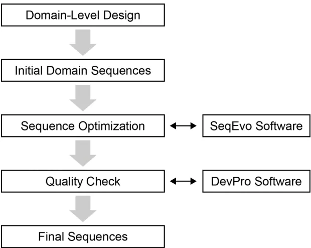
In this dissertation, a new method for implementing DNA systems is presented (Figure 1-7 below). Briefly described, this process starts after the “abstract design” stage. This abstract design is translated into a domain-level design.15 At this stage, each strand in the system is described using only binding domains and their complements. Each of the domains in this design are declared as either variable or fixed and given initial
sequences. Next, the sequence of variable domains are manipulated in order to optimize a fitness metric. This process has been automated using the custom-written Sequence Evolver software (abbreviated SeqEvo). The quality of the system produced by SeqEvo is then scrutinized, and if necessary SeqEvo parameters are tuned and sequence
Figure 1-7 Visual summary of the proposed process for generating DNA systems. Two software tools have been created to help automate this process: the Sequence-Evolver (abbreviated SeqEvo) software for generating in silico optimized sequences,
and the Device Profiler (abbreviated DevPro) software for generating detailed reports characterizing existing systems.
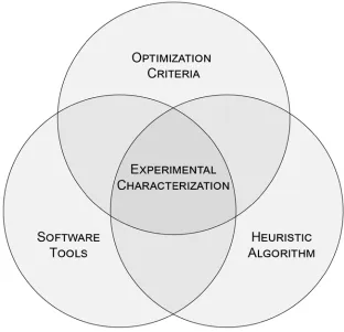
The work in the dissertation is composed of three major efforts, each of which is interdependent to the other two (Figure1-8 below). First, three new criteria for identifying systems with uniform behavior are proposed and studied (Figure 1-8 top). In order to evaluate the performance of these metrics, a robust heuristic algorithm for generating fit sequences was developed (Figure 1-8 right). Creation and optimization of this evolution-inspired algorithm became the second major effort. The development of the algorithm and fitness criteria necessitated the creation of two software tools (Figure 1-8 left). The creation of software tools efficient enough to both characterize and engineer large state-of-the-art DNA systems became the third major effort. Collectively, the new optimization criteria, the new sequence generation algorithm, and the efficient software
of non-target structures (Figure 1-8 center). This enabled us to test the hypothesis that small non-target B-DNA structures are responsible for previously observed kinetic variation. The results of this study both validate that the software/algorithm/criteria are functioning as intended and that their combination represents an improvement over current state-of-the-art methods.
Figure 1-8 Key aspects of this dissertation and their interrelationships. (top) Three new optimization criteria were developed. (left) Two new software tools were
created. (right) A new sequence generation algorithm was developed. (center) The optimization criteria, heuristic algorithm, and software tools were used to generate
CHAPTER TWO: QUANTIFYING SEQUENCE FITNESS In order to reliably generate high-quality DNA systems via sequence
optimization, it is first necessary to know what to optimize. Typically, one would like to have a property which is both simple for a computer to calculate and correlates strongly with a desired measure of performance. Such a property could serve as a metric or criterion for comparing the fitness of systems in silico and facilitate the automated generation of systems with a desired performance. Towards this goal, three new properties quantifying system fitness were proposed and investigated.
Section 2.1 – Quantifying Variations in Dynamic Behavior
One measure of dynamic behavior in DNA systems is the reaction rate of a specific target reaction. Consequently, one measure of behavior variation is the
From these two manuscripts, three experimentally-consistent datasets were extracted. In the first publication, Hata et al. demonstrated that thermodynamically unfavorable structures exhibit a marked impact on reaction rates.37 To support this argument, the authors reported duplex formation rates for 47 implementations of a 23 bp DNA duplex (Figure 2-1b). This set of data was given the label “H25” based on the fact the data was collected at 25°C. The 47 rates reported were all measured under consistent experimental conditions and varied from 1.03 x 10⁴ M-1s-1 to 4.8 x 10⁶ M-1s-1 (Figure
2-1d). In the second publication, Zhang et al. created a model for predicting reaction rates based on similarity to the rates of already measured strand sequence.36 The researchers reported duple-formation rates for 99 implementations of a 36 bp DNA duplex (Figure 2-1c). From this publication, two sets of data were extracted: 99 rate/sequence pairs
Figure 2-1 (a) Flow chart of typical design process with feedback from experimental characterization to implementation process highlighted. (b) Hata et al.
studied the formation rates of 47 implementations of a 23-bp duplex at a temperature of 25°C.37 (c) Zhang et al. studied the formation rates of 99 implementations of a 36 base-pair duplex at temperatures of 37°C and 55°C.36 (d) Reaction rates reported in the three data sets presented as points and summarized by a median line, a box connecting the 25th and 75th percentiles, and bars connecting
The behavior of these simple model systems was observed to be highly variable and should be expected to create a host of issues for researchers designing structures from DNA. For structural systems such as DNA-Bricks or DNA Origami, this should lead to variation in strand incorporation, ultimately impacting both production rates and yields. For dynamic systems such as chemical reaction networks, this directly impacts device performance and presents as massive variation in reproducibility from implementation to implementation.
Section 2.2 – Quantifying Non-Target B-DNA Structures Using Network Fitness
Score, Strand Fitness Score and Total Fitness Score
To quantify the presence of non-target B-DNA type structures, three fitness scores are proposed. Consider again the model system presented earlier (Figure 2-2a below). For this model system, the “complete” list of intermolecular and intramolecular B-DNA structures can be calculated by exhaustively considering all potential base pairings. These lists are “complete” in the sense that they contain all structures, including those that exist as a part of a larger structure. These lists can be summarized by binning structures based on their length and reporting the count of each structure-length (Figure 2-2b and c). The total number and length of structures are further quantified by assigning a score of 10L
as the Total Fitness Scores (TFS, Figure 2-2f). Based on these definitions, NFS can be thought of as a single number quantifying the ensemble of all non-target structures. For this number, lower values correspond to “better” systems and an NFS of zero corresponds to a hypothetical system containing no non-target structures. Similarly, SFS can be
thought of as a number summarizing the ensemble of intramolecular non-target structures. Finally, since intramolecular structures are a subset of intermolecular structures, the TFS can be interpreted as a single number quantifying all non-target structures but with emphasis placed on the intramolecular structures. The intensity of the emphasis is controlled by the ratio of the two scoring weights (C1 and C2 in Figure 2-2f).
Figure 2-2 Calculation of Network Fitness Score (NFS), Strand Fitness Score (SFS), and Total Fitness Score (TFS). (a) Sequences from the model system presented in Figures 1-5. (b,c) Structural profiles summarizing the “complete” sets of intermolecular and intramolecular structures. (d,e) Calculation of NFS, SFS. (f)
TFS is calculated as a weighted linear combination of SFS and NFS. By manipulating the C1 and C2 weights, TFS can be tuned to emphasize either NFS or
SFS.
Section 2.3 – Do B-DNA Structures Explain Kinetic Variation?
in reaction rates in a manner which is both robust to outliers and aligned with the
objective of engineering systems with uniform performance. For this metric, larger values correspond with better kinetic reproducibility.
Method and Results
Figure 2-3 Effectiveness of different fitness criteria at identifying kinetically uniform sequences. (a) Cartoon of the criterion evaluation method. (b) Hybridization rates of the fittest systems within each dataset, as judged by one of the four criteria. Three datasets were analyzed: measurements by Hata et al.37 at 25°C (H25), measurements by Zhang et al.36 at 37°C (Z37), and measurements by
Zhang et al.36 at 55°C (Z55). (c) P-values calculated by comparing the fittest
systems to the associated general population (labeled “none”).
distribution. In this study, the resulting P-values (Figure 2-3c above) indicate that only sequences which are SFS-fit are reliably distinct from the general population.
Interestingly, neither the state-of-the-art Sequence-Symmetry nor the NFS selected sequences produced kinetically distinct populations. This was interpreted as evidence that the majority of kinetic deviations in these systems arise from intramolecular B-DNA type structures. While it is likely that the structures leading to kinetic deviation are
intramolecular in nature, each intramolecular structure logically implies the existence of intermolecular structures. As such, it is important to note that this is evidence of
correlation but not necessary causation. Consequently, it is clear that systems containing fewer intramolecular structures have more uniform kinetics, but it is not necessarily clear why.
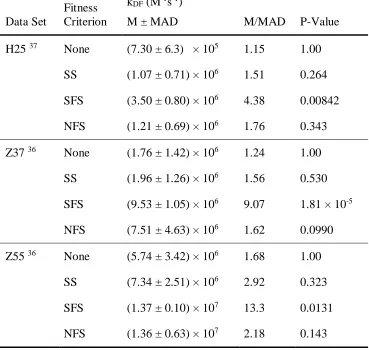
dataset were observed to have an M/MAD ratio of 4.38, corresponding to typical kinetic variation of ± 22.8%.
Table 2-1 Select properties of the fittest systems in each criterion/dataset combination. Reported values include: the duplex-formation rate kDF, the median rate (M), the Median-Absolute-Deviation of rates (MAD), and P-values calculated using a two-sample Kolmogorov-Smirnov test.
Data Set
Fitness Criterion
kDF (M-1s-1)
M ± MAD M/MAD P-Value
H25 37 None (7.30 ± 6.3) × 105 1.15 1.00
SS (1.07 ± 0.71) × 106 1.51 0.264 SFS (3.50 ± 0.80) × 106 4.38 0.00842 NFS (1.21 ± 0.69) × 106 1.76 0.343
Z37 36 None (1.76 ± 1.42) × 106 1.24 1.00 SS (1.96 ± 1.26) × 106 1.56 0.530
SFS (9.53 ± 1.05) × 106 9.07 1.81 × 10⁻⁵
NFS (7.51 ± 4.63) × 106 1.62 0.0990 Z55 36 None (5.74 ± 3.42) × 106 1.68 1.00
SS (7.34 ± 2.51) × 106 2.92 0.323 SFS (1.37 ± 0.10) × 107 13.3 0.0131 NFS (1.36 ± 0.63) × 107 2.18 0.143
In addition, the effectiveness of TFS was determined for several combinations of weighting parameters (Figure 2-4). TFS’s with C1/C2 ratios from 10-6 to 106 were studied.
greater than 100, and to be most effective for ratios greater than 10,000. This result can again be explained by a strong correlation between intramolecular B-DNA type structures and kinetic variation.
Figure 2-4 Tuning of the Total Fitness Score (TFS) weighting parameters to achieve statistically significant P-values. Three datasets were analyzed: measurements by Hata et al.37 at 25°C (H25, orange squares), measurements by
Zhang et al.36 at 37°C (Z37, green circles), and measurements by Zhang et al.36 at 55°C (Z55, blue triangles). P-values are the result of a two-sample Kolmogorov-Smirnov test comparing the fittest systems selected by the TFS function with the
associated general population.
Discussion
kinetic reproducibility for SFS-fit and certain TFS-fit systems. The M/MAD values for the SFS systems range between 4.4 and 13, corresponding with kinetic variations of ± 23% and ± 7.7%, respectively. Interestingly, neither the state-of-the-art SS criterion nor NFS selected systems were statistically distinct from the unfiltered general population.
Section 2.4 – Are TFS-Fit Sequences Kinetically Uniform?
While a strong correlation between intramolecular structures and kinetic variation was observed, the analysis of existing data does not necessarily imply that new systems created using these principles will be kinetically uniform. To confirm that engineering systems with minimal intramolecular and limited intermolecular B-DNA type structures leads to kinetic uniformity, twelve new systems were generated and experimentally characterized.
Methods and Results System Generation
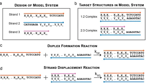
For the purpose of generating fit systems, the SeqEvo software was created. SeqEvo utilizes an evolution-inspired heuristic algorithm to identify systems which are TFS-fit. The TFS weighting parameters supplied to the program can be manipulated to emphasize either SFS-fit or NFS-fit systems. As a design for the model system, three strands capable of undergoing two target reactions were identified (Figure 2-5a below). Two of these strands are fully complementary and contain 41 variable bases (represented with X’s and Y’s such that Xi pairs with Yi in Figure 2-5). This model system design is
2:3). The design is intended to undergo two target reactions. In the first target reaction, Strand 1 and Strand 2 react to form a 49 base-pair B-DNA structure (Figure 2-5c). In the second reaction, Strand 1 interacts with the single-stranded region in complex 2:3 to displace strand 2 and form the 1:3 complex (Figure 2-5d). This mechanism is known as toehold-mediated strand displacement.38 The design is such that the 8 bases utilized in
this reaction are of fixed sequence (5-TCTCCATG-3 and 5-CATGGAGA-3). This was done to eliminate kinetic variation in the strand-displacement reaction known to occur based on toehold sequence.27
Figure 2-5 A model system for studying the impact of non-target structures on reaction kinetics. (a) Three strands compose the model system. (b) The two target
structures in the model system. (c) Schematic of the duplex-formation target reaction. (d) Schematic of the strand-displacement target reaction.
From these variable sequences, strands were compiled and are reported in Appendix A.1. The generated systems were organized into four design groups: three implementations generated via a pseudo-random number generator (RND group), three implementations with the TFS property optimized (TFS group with C1 = 1, C2 = 1), three implementations
with the SFS property optimized (SFS group with C1 = 1, C2 = 0), three implementations
with the NFS property optimized (NFS group with C1 = 0, C2 = 1). These weighting
parameters were chosen based on a binary on/off mentality intended to identify whether (a) these TFS weights would be effective for the target system and (b) whether
optimization of solely SFS or solely NFS would result in kinetic reproducibility. It is important to note that the SeqEvo software results in sequences with two relevant
Figure 2-6 Variable sequences for the twelve systems generated to implement the model system design presented in Figure 2-5. A full list of strand sequences is
provided in appendix A.1.
Generated Systems
The non-target structures in twelve systems were characterized using DevPro and are reported as interference profiles in Figure 2-7 below. The resulting structural profiles were found to be categorizable into three distinct shapes: (1) implementations generated in the NFS and TFS design groups, which contain neither intramolecular structures longer than 2 bp or intermolecular structures longer than 4 bp; (2) implementations generated in the SFS design group, which contain no intramolecular structures longer than 2 bp, but intermolecular structures up to 10 bp in length; and (3) implementations generated in the RND design group, which contain substantial numbers of both
design group contain, on average, approximately 10% fewer intramolecular structures than the NFS design group.
Figure 2-7 Structural profiles of the twelve generated systems. (a) Intermolecular (left) and intramolecular (right) profiles of the three randomly generated systems. (b) Profiles of the three TFS-fit sequences. (c) Profiles of the three SFS-fit sequences.
(d) Profiles of the three NFS-fit sequences. These structural profiles are complete in the sense that they contain all non-target structures, including those which exist
Experimental Characterization
The behavior of the twelve generated systems were characterized by monitoring reactant concentration in real time using fluorescence measurements. This technique is illustrated in Figure 2-8 below using the TFS-1 system (Figure 2-8a) at 20°C as an example. First, strands were purchased from Integrated DNA Technologies
Figure 2-8 Method for experimentally characterizing reaction kinetics. (a) One of the generated systems for use as an example. (b) Dye/quencher functionalized strands were prepared at pre-determined experimental conditions. (c) Sample fluorescence was monitored in real-time. (d) Plot of inverse strand concentration vs elapsed time. (e,f) Linear fits applied to all data preceding reaction half completion
in d.
Kinetic Modeling
Both the duplex-formation and strand displacement reactions (Figure 2-5c,d) were modeled as bimolecular and irreversible (equation 1 below).
𝐴𝐴+𝐵𝐵 → 𝐶𝐶𝑘𝑘 1
For this reaction, the law of mass action dictates that the rate of reactant consumption and the rate of product creation are equal (eq. 2).
𝑑𝑑[𝐴𝐴] 𝑑𝑑𝑑𝑑 =
𝑑𝑑[𝐵𝐵] 𝑑𝑑𝑑𝑑 =−
𝑑𝑑[𝐶𝐶]
As such, the assumption that reactants are initially at equal concentrations (stoichiometry) implies that the reactant concentrations remain equal indefinitely.
[𝐴𝐴]0 = [𝐵𝐵]0 3
[𝐴𝐴] = [𝐵𝐵] 4
Substitution and rearrangement of eq. 2 allows separation of variables in eq. 5.
−𝑑𝑑[𝐴𝐴[𝐴𝐴]2]= 𝑘𝑘𝑑𝑑𝑑𝑑 5
Integration of eq. 5 yields a linear relationship between the inverse reactant concentration and time.
1
[𝐴𝐴] =𝑘𝑘𝑑𝑑+𝐶𝐶 6
Based on this model, one can expect a plot of inverse concentration vs time to be linear for any stoichiometric, bimolecular, and irreversible reaction. For both duplex formation and strand displacement reaction, these plots were observed to be approximately linear for times prior to half completion (Figure 2-8d above). Nonlinear behavior was observed beyond half completion. This is consistent with the increasing deviation from
stoichiometry which is expected for such reactions. The slope of the linear region is equal to the bimolecular rate constant k, which was extracted using a linear fit to the data (Figure 2-8e, f).
Measured Reaction Rates
One hundred and fifty-two total reaction rates were experimentally determined. For each of the twelve implementations (RND-1, RND-2, RND-3, TFS-1, TFS-2, TFS-3, SFS-1, SFS-2, SFS-3, NFS-1, NFS-2, and NFS-3), the rate of both target reactions (kDF
Sample preparation and rate measurements were repeated two additional times for the TFS-3 system at 20°C and 40°C for both kDF and kSD. The resulting kDF measurements of
6.1 x 10⁵, 7.0 x 10⁵, 6.7 x 10⁵ M-1s-1 at 20°C and 5.9 x 10⁶, 6.0 x 10⁶, and 5.8 x 10⁶ M-1s-1 at 40°C indicate the precision of this method is such that a single measurement of each rate is reasonably appropriate for the target study. The resulting kSD measurements of 1.5
x 106, 1.8 x 10⁶, 1.5 x 10⁶ M-1s-1 at 20°C and 1.6 x 10⁶, 1.6 x 10⁶, and 1.7 x 10⁶ M-1s-1 at 40°C indicate similar precision for the strand-displacement rates.
The 12 sets of rates determined for the duplex-formation reaction are reported in Figure 2-9. These rates were observed to span five orders of magnitude, with rates
ranging from a minimum value of 9.6 x 10³ M-1s-1 (RND-1 at 10 °C) to a maximum value
of 8.0 x 10⁷ M-1s-1 (TFS-1 at 60 °C). The largest range observed at a given temperature resulted from the measurements at 10 °C, which spanned four orders of magnitude from 9.6 x 10³ M-1s-1 to 3.7 x 10⁶ M-1s-1 (RND-1 and SFS-1, respectively). Duplex formation M/MAD ratios were calculated for each design-group at each temperature yielding average ratios of 1.5, 19.7, 5.5, and 4.4 for the RND, TFS, NFS and SFS groups, respectively. The largest duplex formation M/MAD ratio observed was a value of 44 (TFS group at 30 °C). The smallest M/MAD ratio observed was a value of 1.4 (RND group at 40 °C). The majority of rate/temperature profiles were observed to be well described by an Arrhenius model (equation 7 and Figure 2-10 below) relating the kinetic rate (k) to an activation energy (Ea), a pre-exponential factor (A), the Boltzmann constant
(kb), and the temperature (T).
𝑘𝑘 =𝐴𝐴exp�−𝐸𝐸𝑎𝑎
𝑘𝑘𝑏𝑏𝑇𝑇� 7
reaction rates as a function of inverse temperature yielded the Arrhenius slope, intercept and R2 values reported in Table 2-2 below.
Figure 2-9 Experimentally determined duplex-formation (kDF) rates for the
twelve implementations of the model system. The discrete data points are connected by lines to aid the eye. Experiments were performed in triplicate for the TFS-3 system at 20 °C and 40 °C. The error bars on these data points span from the mean
Figure 2-10 Arrhenius fits to the experimentally determined duplex-formation (kDF) rates for the twelve implementations of the model system. Discrete data points
Table 2-2 Arrhenius parameters extracted from the duplex-formation rates (kDF) of each implementation. The activation energy (Ea), pre-exponential factor (A), and R2 of the Arrhenius fit are reported.
Arrhenius Parameters
Sequence Set Ea (10-19 J) A (M-1s-1) R2
RND-1 1.71 1.41 x 10²³ 0.995
RND-2 1.10 1.42 x 10¹⁸ 0.985
RND-3 1.68 1.72 x 10²³ 0.989
TFS-1 1.38 7.75 x 10²⁰ 0.993
TFS-2 1.36 3.15 x 10²⁰ 0.992
TFS-3 1.42 1.16 x 10²¹ 0.998
SFS-1 0.654 1.18 x 10¹⁴ 0.861
SFS-2 1.24 1.73 x 10¹⁹ 0.962
SFS-3 1.50 7.73 x 10²¹ 0.997
NFS-1 1.28 4.27 x 10¹⁹ 0.993
NFS-2 1.57 1.56 x 10²² 0.992
NFS-3 1.82 6.94 x 1024 0.988
The strand-displacement rates measured for each device are reported in Figure 2-11 below. Strand displacement reactions were observed to systematically deviate from the bimolecular model such that the reactant consumption slowed as elapsed time
simple bimolecular model are that it is based on a single kinetic rate and adequately quantifies system behavior such that behavior variation can be studied. More specifically, if systems have uniform dynamic behavior one would expect them to be have similar apparent bimolecular rates, regardless of the fact that model is an over simplification. Measured strand displacement rates were observed to be less variable than the duplex-formation rates; the maximum and minimum rates spanned 3 orders of magnitude and ranged from 1.9 x 10⁴ M-1s-1 (RND-1 at 10 °C) to 1.9 x 10⁶ M-1s-1 (SFS-2 at 30 °C).
This trend can potentially be explained by two factors: (1) several bases in the 2:3
complex are already in a B-DNA type structure, potentially eliminating their contribution to kinetic variation, and (2) the strand displacement reaction is designed to proceed through a specific reaction pathway including toehold formation, potentially eliminating kinetic variation arising from alternative reaction pathways. Strand displacement
Figure 2-11 Experimentally determined strand-displacement rates for the twelve implementations of the model system. Experiments were performed in triplicate for the TFS-3 system at 20 °C and 40 °C. The error bars on these data points span from
Discussion
Several trends in the experimentally characterized rates provide important insight into the relationship between non-target structures and kinetic variation. First, rates for both reactions are observed to be highly sequence-dependent. Indeed, it is observed that variation of sequence alone leads to rates spanning up to four or three orders of
magnitude for the duplex-formation and strand-displacement reactions, respectively. For the duplex-formation reaction, kinetic variations of this magnitude have been observed previously, with the data reported by Hata et al. and Zhang et al. similarly spanning up to four orders of magnitude.36,37 In addition, our observation of strand-displacement rate variation is consistent with the variations observed by Olson et al. while studying the impacts of sequence variation on chemical reaction network dynamics.54 In addition, a study by Zhang and Winfree demonstrated that variation in toehold sequence and size can lead to strand-displacement rates varying up to seven orders of magnitude.27 The results of this study expand upon this finding, making it clear that even systems with fixed toeholds vary by up to three orders of magnitude. This type of variation may also help explain the deviations from the three-step model observed by Zhang and Winfree for toeholds with high thermodynamic stability.
observation that most systems exhibit similar Arrhenius behavior suggests that reaction mechanisms are largely preserved regardless of non-target structures. These findings are consistent with the nucleation-and-zipper model of duplex-formation described by
equation 8 below.55 In this model, nucleated intermediates form based on the bimolecular rate k1f. These nucleated intermediates either dissociate back into reactants or proceed to
reaction completion based on the unimolecular rate constants k1r or k2, respectively.
Based on the steady-state approximation, such a reaction results in an apparent
bimolecular kinetic rate (kapp) described by equation 9. Insufficient evidence is observed
in the data to speculate if the Arrhenius barrier observed for bimolecular duplex-formation rates arises from a single or multiple Arrhenius barriers in k1f, k1r and k2.
A + 𝐵𝐵𝑘𝑘⇄1𝑓𝑓 𝑘𝑘1𝑟𝑟
AB†𝑘𝑘→2𝐴𝐴𝐵𝐵 8
𝑘𝑘𝑎𝑎𝑎𝑎𝑎𝑎 = 𝑘𝑘1𝑓𝑓
1 +𝑘𝑘1𝑟𝑟 𝑘𝑘2
9
The values of the Arrhenius activation energy (Ea) and pre-exponential factor (A)
describing the duplex-formation rates of the 12 implementations are observed to be non-independent and strongly correlated (Figure 2-12 below). The correlation is such that a plot of the natural logarithm of A as a function of Ea appears linear in nature (eq. 10
below). Such relationships in DNA have been previously reported in the literature, and were interpreted as a consequence of the underlying linear free energy relationship.57 This observation was confirmed using a linear fit (red line in Figure 2-12) resulting in an R2 value of 0.9889, an intercept of 19.4 (a in eq. 10 below), and a slope of 2.05 x 10²⁰ (b
in eq. 11). Following the combination of equations 1 and 3, the declaration of constants C and Tc (eq. 11), and algebraic rearrangement, an empirical kinetic model can be derived
(eq. 12). This model suggests that the duplex formation rates of the 12 devices are largely explainable based on two variables (Ea and T), and three constant parameters (C, Tc, and
kb). One interesting feature of this kinetic model is the critical temperature parameter Tc,
which can be interpreted as a hypothetical critical temperature at which device kinetics should be uniform and equal to the pre-exponential constant C. The linear fit of the Arrhenius parameters predicts values of 82 °C and 2.7 x 10⁸ M-1s-1 for T
c and C,
ln(𝐴𝐴) =𝑎𝑎+𝑏𝑏 ∙ 𝐸𝐸𝑎𝑎 10
𝐶𝐶 ≡exp(𝑎𝑎) 𝑇𝑇𝑐𝑐 ≡ 𝑘𝑘1
𝑏𝑏∙ 𝑏𝑏 11
𝑘𝑘= C∙exp�𝐸𝐸𝑘𝑘𝑎𝑎 𝑏𝑏�
1 𝑇𝑇𝑐𝑐 −
1
𝑇𝑇�� 12
Figure 2-12 Observed correlation between the natural log of the Arrhenius pre-exponential (vertical axis) and the Arrhenius activation energy (horizontal axis). A linear fit to the data (red line) resulted in an R2 value of 0.9889, an intercept of 19.4,
Figure 2-13 Experimentally determined duplex-formation rates (symbols) modeled using the empirically derived kinetic model reported in the text (dashed
lines).
found to only exhibit this parabolic behavior when they contain no intramolecular structures longer than 2 bp. Based on this observation, it was concluded that
intramolecular structures lead to a change in the rate-limiting mechanism of the reaction leading to two distinct behaviors: (1) an approximately linear region at low temperatures with positive slope, and (2) an approximately linear region at high temperatures with negative slope. Both behaviors can be explained by a kinetic model where reactants form a stable intermediate which may then either proceed to reaction completion or dissociate. The mathematics of such a model are identical to the nucleation-and-zippering model of DNA duplex formation described in equations 8 and 9 above, albeit with varying physical interpretation of the relevant rate constants. In the case of the strand-displacement
reaction, the stable intermediate is a three stranded complex and this complex proceeds to completion via the strand-displacement step. If the dissociation rate of the intermediate (k1r) is much smaller than the rate at which the intermediate is converted into products
(k2), then kapp is approximately the duplex-formation rate of the toehold (k1f). Based on
the temperature-profile of the measured duplex-formation rates (Figure 2-9), it is reasonable that these rates may be Arrhenius with positive slope and thus explain the observed low-temperature behavior.
In addition, strand displacement rates (kSD) were observed to converge at higher
temperatures, and have negative slopes. This behavior can be explained based on the same kinetic model (Eq. 8, 9) if the rate of intermediate dissociation (k1r) is much larger
than the rate of intermediate conversion (k2). This leads to apparent bimolecular rates
(kSD) which take the form of equation 13 below. Furthermore, modeling each of the three
reaction rate which is itself Arrhenius and possesses an activation energy (Ea,SD) equal to
the difference in energies of the three barriers (eq. 14). In such a situation, a large energy barrier to intermediate dissociation (Ea,1r) may dominate the apparent energy barrier
(Ea,SD) and lead to kinetics which depend almost exclusively on this value. This can be
expected to result in rates which decrease as temperature increases and which depend strongly on toehold sequence, a variable held constant in these systems. The parabolic behavior can thus be described as a transition between the first behavior at low
temperature and the second behavior at high temperature.
𝑘𝑘𝑆𝑆𝑆𝑆 = 𝑘𝑘𝑘𝑘1𝑓𝑓
1𝑟𝑟𝑘𝑘2 13
E𝑎𝑎,𝑆𝑆𝑆𝑆 = E𝑎𝑎,1𝑟𝑟− �E𝑎𝑎,1𝑓𝑓+ E𝑎𝑎,2� 14
For both reactions studied, systems in the TFS design group exhibited the greatest kinetic reproducibility (Figure 2-14). For the duplex-formation reactions (Figure 2-14a), TFS-fit sequences were observed to possess temperature averaged M/MAD ratios of 19.4, corresponding with typical kinetic variations of ± 5%. For the strand-displacement reactions (Figure 2-14b) these devices exhibited temperature averaged M/MAD ratios of 9.1, corresponding to typical kinetic variations of ±11%. It is also evident that for
Figure 2-14 Kinetic reproducibility of the TFS-optimized implementations compared to the unoptimized RND implementations. (a) M/MAD ratios calculated from the duplex formation (kDF) rates. (b) M/MAD ratios calculated from the strand
displacement (kSD) rates.
Section 2.5 – Further Discussion
DNA molecules have been previously shown to form numerous structures other than the A/T and G/C base pairs and resulting B-DNA double helix.17 However, the results from this study indicate that the absence of intramolecular non-target B-DNA type structures results in DNA systems with highly reproducible kinetic rates. This surprising result suggests that although many alternative structures may form, B-DNA type
structures are the primary contributor to kinetic variation. It is further observed that intramolecular structures as short as 3 bp exhibit a marked impact on reaction kinetics. Conversely, no experimental or theoretical evidence is observed linking small
intermolecular structures to kinetic variation. The ability of large intermolecular
demonstrated in the strand displacement rates measured for the model system. However, SFS-fit systems selected from the Zhang et al. and Hata et al. datasets contain
intermolecular complements from 3 to 7 bp in length yet remain kinetically uniform. This demonstrates that intermolecular structures up to this length can exist in DNA systems without substantially impacting reaction kinetics. As such, further study is necessary to establish under what conditions (i.e., length, location, and frequency) intermolecular structures will impact reaction kinetics.
using the new TFS criteria should therefore be expected to be substantially more reproducible than systems generated using current state of the art methods.
Evaluating sequence-set fitness using TFS has several key advantages relative to alternative methods. First, since TFS calculation is based solely on strand sequence without accounting for experimental conditions, sequence-sets which are TFS-fit are expected to perform similarly at a range of experimental conditions including
temperature, buffer, and ion concentration. Second, calculating TFS does not require computation of thermodynamic parameters for the system making this method computationally efficient by comparison. Equivalently, this enables more potential systems to be considered in a fixed unit of time relative to thermodynamic approaches.
However, evaluating the fitness of DNA systems using TFS also has several key limitations. Foremost, it is clear that not all structures impact reaction kinetics equally. As such, TFS penalizes a number of systems which are kinetically-fit, yet contain
non-problematic structures. Secondly, TFS penalizes systems based on the length of structures, this is based on the approximation that structure stability is based solely on length. For small structures, this approximation is not bad, however it degrades quickly as length scales. It is assumed that this will impact the effectiveness of TFS for systems which necessitate the inclusion of larger structures.
Section 2.6 – Conclusions
engineering DNA systems to eliminate all non-target intramolecular B-DNA structures longer than 2 bp leads to kinetically uniform reaction rates. Engineering systems such that intramolecular structures larger than 2 bp are eliminated and intermolecular