Article
1
Pressure detrending in Harmonic Pulse Test
2
interpretation: when, why and how
3
Dario Viberti 1,*, Eloisa Salina Borello 2 and Francesca Verga 3
4
1 Politecnico di Torino; [email protected]
5
2 Politecnico di Torino; [email protected]
6
3 Politecnico di Torino; [email protected]
7
* Correspondence: [email protected]; Tel.: +39-011-090-7731
8
9
Abstract: In reservoir engineering, one of the main sources of information for the characterization
10
of reservoir and well parameters is well testing. Among the unconventional well testing
11
methodologies, Harmonic Well Testing (HPT) is appealing from an economic standpoint because it
12
could provide well performance and reservoir behavior monitoring without having to interrupt
13
field production. Recorded pressure analysis is performed in the frequency domain by adopting a
14
derivative approach similar to conventional well testing. To this end, pressure and rate data must
15
be decomposed into harmonic components. Test interpretability can be significantly improved if
16
pressure data are detrended prior to interpretation, filtering out non periodic events such as
17
discontinuous production from neighboring wells and flow regime variations which did not respect
18
the designed test periodicity. Therefore, detrending offers the possibility of overcoming the
19
limitation of HPT applicability due to the difficulty of imposing a regularly pulsing rate for the
20
whole test duration (typically lasting several days). This makes HPT attractive for well performance
21
monitoring, especially in gas storage fields. In this paper, the application of different detrending
22
methodologies to synthetic HPT pressure data generated in different reservoir and operational
23
scenarios is presented and discussed. Moreover, a real case application is also presented.
24
Keywords: well testing, detrending, harmonic pulse testing, well performance monitoring,
25
underground gas storage
26
27
1. Introduction
28
Broadly speaking well testing provides pressure measurements which are mainly used for
29
determining reservoir-rock properties and producing-formation limits and as such it is considered
30
an effective method of reservoir analysis. Conventional well tests have been used by reservoir
31
engineers to evaluate well and reservoir performance for decades (([1–5]); by doing they aim at
32
reducing uncertainty as much as possible in addition to trying to understand that part which cannot
33
be reduced. Over the last years, work has focused on developing unconventional or, perhaps more
34
accurately, complementary well test methodologies that are both less expensive and more
35
environmentally friendly procedures ([6–14]).
36
These complementary well test methodologies can prove reliable alternatives to obtaining a
37
reasonable amount of information when conventional well testing cannot be applied. Among the
38
complementary well testing methodologies, Harmonic Pulse Testing (HPT) is appealing from an
39
economic standpoint as it can provide well performance and reservoir monitoring without having to
40
interrupt field production. In HPT a pulsed signal is superimposed to the background pressure trend;
41
thus no interruption of well and reservoir production is required before and during the test.
42
Simple Pulse testing as a methodology for reservoir properties characterization dates back to
43
1966 when it was first proposed by Johnson et al. ([15]). Since then, theoretical developments have
44
led to the current characteristic of periodicity of the original test procedure which allows the
45
application of interpretation methodology in the frequency domain ([16–33]). Thus, a harmonic test
46
is that in which the injection or production rate is varied in a periodic way. These rates can be imposed
47
after a long shut in of the tested well, like in conventional well testing, or they can be superposed to
48
ongoing production and without interrupting the production activities from other wells, hence the
49
economic benefit of the methodology. However, HPT does show a limitation in terms of the
50
investigation distance, which is shorter for the same test duration as compared to that of a
51
conventional well test. Additionally, reliable test interpretation means regular sampling of the
52
pressure data and reasonable periodicity of the imposed rate signal. Despite the aforementioned,
53
HPT methodology and interpretation does not require the initial static pressure nor the previous
54
production history of the well which in turn are considerable advantages ([33]).
55
Pressure and rate signals recorded during HPT are first analyzed in the frequency domain with
56
proper methodologies, mainly based on Fourier Analysis, to then be interpreted by adopting a
57
derivative approach similar to that of a conventional well test [33]. Pressure data should be
58
adequately pre-processed with detrending methodologies to separate pure periodic components of
59
the signal from non-periodic components; in this way the information obtained from HPT
60
interpretation can be maximized. First transient magnitude, discontinuous production from
61
neighboring wells, flow regime variations, etc. produce a significant non-periodic component in the
62
pressure response which might strongly affect the periodicity of the pressure signal and hence the
63
reliability of test interpretation.
64
To filter out non-periodic components different detrending approaches have been suggested in
65
the literature: for instance, Hollaender ([20]) adopted a polynomial reconstruction of the aperiodic
66
depletion trend; and more recently detrending approaches based on a heuristic reconstruction of a
67
constant depletion have been presented ([25], [34]).
68
In the present paper, four detrending methodologies (method 0, method 1, method 2 and
69
method 3 hereinafter) are considered and discussed. Method 0 is the simple linear detrending.
70
Method 1 is an interesting and efficient heuristic algorithm proposed by Ahn and Horne ([35]).
71
Methods 2 and 3 ([34]) are heuristic algorithms developed by the authors in steps, initially with the
72
aim of overcoming some limitations of the Ahn and Horne algorithm, and subsequently to extend
73
the approach to any possible scenario as well as to better characterize the periodic and the
non-74
periodic components.
75
The four detrending algorithms were applied to several synthetic cases representative of
76
possible scenarios and to a real gas storage case. The resulting detrended harmonic signals were
77
analyzed in the frequency domain adopting the approach presented by Fokker et al. ([33]) and
78
compared in terms of quality of the harmonic components derivative and interpretation results.
79
Furthermore, the four detrending algorithms were applied to a real case in which temporarily
80
test interruptions due to operational constraints negatively affected pressure response periodicity.
81
2. Results
82
In order to validate and compare the presented detrending methodologies, several synthetic
83
cases were generated. Each case represents a different scenario characterized by both reservoir
84
behavior and production operations or events that can potentially affect the test. From a reservoir
85
behavior viewpoint, three main scenarios were considered:
86
• Simple homogeneous system
87
• Presence of one boundary within the investigated area of the test
88
• Closed system with high depletion
89
From a production operations or events viewpoint, several possible situations were taken into
90
account:
91
• Interfering well produced with constant rate
92
• Interfering well production with rate variation longer than the oscillation period
93
• Interfering well production with rate variation shorter than the oscillation period
94
• Complex historical productions (preceding the test) not available for the interpretation. Only
96
the value of the last rate before the test is known.
97
In all scenarios, the use of a detrending algorithm proved valuable to improve data quality and
98
hence test interpretation. A selection of the scenarios is described in detail in the following sections
99
3.1 - 3.4 of this paper. The common data adopted for the generation of synthetic cases are summarized
100
in Tab. 1; pressure and rate data are generated with a constant sampling interval of 10 s. The rates
101
adopted to impose the harmonic oscillation will be indicated as q1 and q2, whereas q0 refers to the last
102
historical rate prior to the HPT. The rate is obviously null when initial static conditions are simulated
103
at the beginning of the test.
104
In addition, a real gas well HPT was analyzed; the test was interrupted twice for several hours
105
because of operational constraints, thus inducing two considerable irregularities in the pressure
106
periodical trend.
107
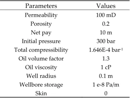
Tab. 1: Common data adopted for synthetic case generation.
108
Parameters Values
Permeability 100 mD
Porosity 0.2
Net pay 10 m
Initial pressure 300 bar Total compressibility 1.646E-4 bar-1
Oil volume factor 1.3
Oil viscosity 1 cP
Well radius 0.1 m
Wellbore storage 1 e-8Pa/m
Skin 0
2.1 Synthetic case 1: ideal condition
109
The first selected case presents ideal conditions to preserve the periodic trend of pressure
110
response. Production starts from the initial static conditions. The test consists of seven oscillating
111
cycles in which constant production of q1=800 m3/day is alternated with shut in of q2=0 m3/day every
112
24 hours (Fig. 1a).
113
114
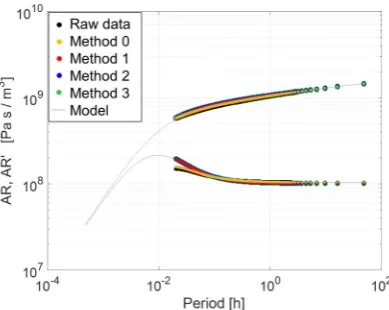
(a) (b)
116
Fig. 2: Derivative in the frequency domain.
117
Neither well interference nor significant overall pressure decline are imposed. Moreover, the
118
influence of the initial transient is very limited because q2 = q0. Therefore, the derivative of raw data
119
is interpretable only because high frequency harmonics (T< 0.1h) are affected (Fig. 2).
120
Linear detrending is not well suited to remove the initial transient effect (Fig. 1b). On the
121
contrary, the adoption of any of the heuristic detrending strategies presented in section 4 improves
122
the pressure data (Fig. 1b) and, in turn, the derivative for high frequency components (Fig. 2). Notice
123
that in this case derivatives obtained from detrended data with methods 1, 2 and 3 perfectly overlap.
124
2.2 Synthetic case 2: depletion
125
In the second case, strong reservoir depletion is simulated by considering a closed reservoir of
126
1000 m x 1000 m with the pulser at the center and introducing a second well (well 1) at a distance of
127
150 m from the pulser. The additional well is produced with a constant rate of 2000 m3/day.
128
The production from the pulser and from well 1 starts simultaneously and from the initial static
129
conditions. The test is made up of five oscillating cycles in which rates are alternated every 24 hours
130
between q1=600 m3/day and q2=500 m3/day (Fig. 3a).
131
Two effects mask the periodic trend under the described pressure profile: the depletion trend
132
and a pronounced initial transient. In fact, being q0 ≠q2, the magnitude of the first pressure transient,
133
corresponding to the first hemicycle (from 0 to ), is significantly higher than the following pressure
134
oscillations; the more q0 differs from q2, the more the initial transient masks the periodic trend in
135
pressure data.
136
137
(a) (b)
Fig. 3: Synthetic case 2: (a) imposed rate and pressure response; (b) detrended pressure data.
138
All the detrending strategies presented in section 4 were applied; the obtained detrended
139
amplitude ratio of harmonic components of the pressure and rate spectrums and their derivative
141
(referred to as derivative hereinafter) with respect to the oscillation period are represented. The
142
results obtained for raw data and for the pressure data processed with methods 0, 1, 2 and 3 are
143
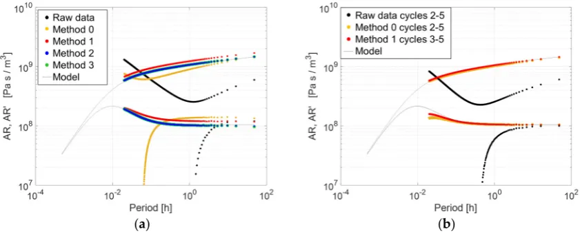
represented Fig. 4a.
144
The analysis of the log-log plot (Fig. 4a) shows that the derivative of the raw data and of method
145
0 detrended pressure do not provide reliable interpretation for both high frequencies (low T values)
146
and low frequencies (high T values). Significant errors in the estimation of the kh (underestimation
147
of 25%) and of the skin (S=-2.5 instead of 0) are observed. The derivative of method 1 detrended
148
pressure is affected, as expected, by the first transient and would induce an underestimation of kh of
149
10% and a slightly incorrect evaluation of mechanical skin (S=0.5 instead of 0). However, both
150
approaches are still applicable if the number of oscillating cycles is high enough (which is rarely the
151
case in real applications) to allow removing the first cycle, which is strongly influenced by initial
152
transient due to q0≠q2 (Fig. 4b). The removal of initial transient is anyhow not sufficient to analyze
153
raw data because the linear trend still masks periodicity.
154
Method 2 and method 3 give very similar results (derivatives overlap), and provide an excellent
155
match with the theoretical model.
156
157
(a) (b)
158
Fig. 4: Derivative in the frequency domain: (a) all cycles; (b) cycles affected by transient excluded from
159
the Fourier analysis.
160
2.3 Synthetic case 3: partially unknown pre-existing history
161
In the third selected case, a single no-flow boundary was defined at a distance of 30 m from the
162
pulser. The well is produced with a changing rate before the test (see Fig. 5a); only the very last
163
production rate (q0=200 m3/day) preceding the test is needed for interpretation purposes . The test is
164
made up of seven oscillating cycles in which rates are alternated every 24 hours between q1=600
165
m3/day and q2=500 m3/day (see Fig. 5a).
166
The periodic trend is masked by the initial transient under this pressure profile.
167
(a) (b)
Fig. 5: Synthetic case 3: (a) imposed rate and pressure response; (b) detrended pressure data.
169
The heuristic detrending strategy presented in section 4 (method 1, method 2 and method 3) was
170
applied and the obtained detrended pressures are compared in Fig. 5b. Moreover, results were
171
compared against raw data in terms of derivative (Fig. 6).
172
The derivative of raw data induces an underestimation of the kh value of 20% and an incorrect
173
evaluation of the mechanical skin (S=-1.5 instead of 0). The derivative of method 1 processed data
174
induces an underestimation of kh of 8% and a slightly incorrect evaluation of mechanical skin (S=-0.4
175
instead of 0). These errors are due to the incorrect detrending of the first cycle, which is strongly
176
influenced by the initial transient due to q0 ≠q2. Methods 2 and 3 provide a reliable derivative
177
(derivatives almost overlap), with a correct identification of the single boundary position.
178
It turns out that only the very last production rate preceding the test (q0) has an impact.
179
Consequently, detrending can be effective if the value of the last production rate prior to the test is
180
known, even so when pre-existing production is complicated.
181
182
Fig. 6: Derivative in the frequency domain.
183
2.4 Synthetic case 4: sudden interference
184
In this case, an interfering well placed at 80m from the Pulser is introduced. The well produces
185
500 m3/day, but a sudden well shut in of 15 h occurs during the test. Both wells produced 500 m3/day
186
before the test (q0=500 m3/day); the test is made up of five oscillating cycles in which rates are
187
alternated every 24 hours between q1=600 m3/day and q2=500 m3/day (Fig. 7a).
188
Notice that, in this case, the pre-existing rate (q0) is equal to the rate of the second oscillation
189
hemicycle (q2); therefore, no initial transient is observed and the first oscillation cycle is in line with
190
the last two cycles. Conversely, the second cycle is highly affected by the rate change in the interfering
191
well.
192
(a) (b)
Fig. 7: Synthetic case 4: (a) imposed rate and pressure response; (b) detrended pressure data.
194
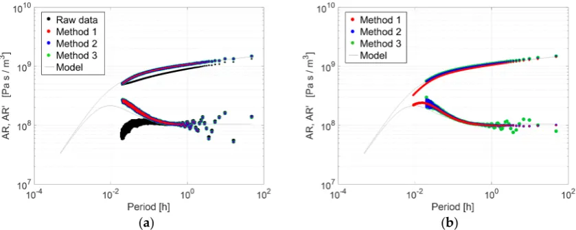
The heuristic detrending strategies presented in section 4 (method 1, method 2 and method 3)
195
were applied; the obtained detrended pressures are compared in Fig. 7b. In this case, the detrended
196
pressure of method 1 and method 2 are similar whereas differ significantly from the detrended
197
pressure of method 3. In fact, with method 2 (similarly to method 1) the irregularity due to the
198
interfering well is marked and affects mainly the second cycle, while with method 3 the irregularity
199
due to the interfering well is less marked because it is spread over two cycles. Results were compared
200
against raw data in terms of derivative (Fig. 8a). It turns out that a rate change in an interfering well
201
lasting less than the oscillation period (or hemicycle) has a strong impact on the derivative, which is
202
highly noisy even at low frequency components; as a consequence the horizontal stabilization
203
representing radial flow geometry in transient regime (Infinite Acting Radial Flow - IARF) is hardly
204
detectable.
205
Successively, the most irregular oscillation period (cycle 2) was excluded from the analysis (Fig.
206
7b) and the improvement in derivative interpretability is shown in Fig. 8b. Notice that method 3 is
207
not well suited for detrending such scenario because it spreads the irregularity over more oscillating
208
cycles, thus making the exclusion of the more affected cycle less effective.
209
(a) (b)
Fig. 8: Derivative in the frequency domain: (a) all cycles; (b) cycle affected by interfering well excluded
210
from the Fourier analysis.
211
2.5 Real case: temporary interruption of the test
212
A gas storage well was tested during the injection campaign without interruption of the activities
213
from the other wells of the field in Italy. The test design was a rate of 250000 m3/day for 24 hours
214
alternated with well shut in of the same duration (Fig. 9a). Significant rate instability/fluctuations
215
was recorded every 10 s while rate data was recorded every 30 s; rate data was resampled according
217
to pressure data. Due to operational issues after the first two cycles the test was temporarily
218
interrupted (well was shut after 1.5 h of injection and remained shut for 13.5h) and was interrupted
219
again for 47.5h (extended well shut in) after the following 1.5 cycle. Consequently, the overall test
220
periodicity was seriously compromised and only few consecutive cycles were available. Except for
221
the two test interruptions aforementioned, in most hemicycles rate changes were
222
anticipated/postponed with respect to the design by a few to a maximum of 40 minutes. As a
223
consequence, the raw test data does not meet the HPT interpretation methodology requirements of
224
regular periodicity. In fact, when applying the Fourier analysis to the original data a scattered
225
derivative is obtained (Fig. 10a), which is clearly not interpretable.
226
All the four detrending techniques described in section 4 were applied to pseudopressure data.
227
Notice that method 0 and method 1 were suitable in this context because q2=q0=0, thus no initial
228
transient was observed. However, detrending with method 0 was not completely successful because
229
the slope of the linear trend changed after the second test interruption.
230
After detrending, the data portion related to the two test interruptions were removed; for
231
method 2 and method 3, which gave more regular oscillations, a further regularization was applied
232
by removing all the data portion related to hemicycle duration greater than the minimum one (23.34
233
h). The detrended pseudopressure data obtained from each methodology is compared in Error!
234
Reference source not found.. Derivatives of detrended data are compared in Fig. 10b. All cases show
235
great improvement and allow kh identification. Among the detrending strategies, method 3 allowed
236
better extraction of early time information. The residual scattering observable on the derivatives for
237
methods 2 and 3 is due to rate instabilities and for methods 0 and 1 to the residual flow period
238
duration irregularity as well.
239
240
(a) (b)
Fig. 9: Real case: (a) imposed rate and pressure response; (b) detrended pseudopressure data with
241
exclusion of main irregularities.
242
Fig. 10: Derivative in the frequency domain: (a) raw data; (b) detrended data.
243
3. Discussion
244
The analyzed cases showed that only in the ideal case of negligible well interference – small
245
overall pressure decline and negligible initial transient (q0 = q2 ) as in synthetic case 1 – the Fourier
246
analysis of HPT raw pressure data is feasible. In fact, in the other considered scenarios (well
247
interference, significant overall pressure decline, initial transient due to previous history) the
248
derivative obtained from raw data analysis in the frequency domain was either not interpretable or
249
the interpretation was not reliable. In such scenarios the use of a detrending algorithm as a data
250
preprocessing is compulsory.
251
The detrending strategies allowed to extract from pressure raw data the periodic component
252
that was masked by non-periodic effects, and thus enhanced the quality of the derivative. Based on
253
the results, the adequate detrending strategies for each scenario are listed below:
254
• in presence of a significant pressure decline, either due to reservoir depletion or constant well
255
interference, all the considered strategies are effective.
256
• if a significant initial transient is observed, because of rate history prior to the test (es. q0 << q2),
257
method 2 or method 3 can be successfully adopted.
258
• if any oscillation cycle (or hemicycle) is significantly altered by an interfering well, method 1 or
259
method 2 can be adopted to allow the exclusion of anomalous cycle(s) from the Fourier analysis.
260
• if any hemicycle is significantly longer/shorter than the design, as in the case of a temporary
261
suspension of the test, detrending with method 1, method 2 or method 3 allows the exclusion of
262
the redundant parts of the hemicycle(s)/the exclusion of the short cycle(s) from the Fourier
263
analysis.
264
4. Materials and Methods
265
Detrending refers to methodologies aimed at removing from a time series any trend that can
266
mask or affect the information of interest. In the case of HPT, detrending refers to recognizing a
non-267
periodic depletion trend and removing it from the pressure signal to isolate the pure periodic
268
component. The four detrending methodologies, discussed in this paper do not require any model or
269
parameter characterization. They are based on the observation of the pressure data only (methods 0
270
and 1, or on the observation of the pressure and rate data (methods 2 and 3), and they try to
271
approximate or reconstruct the non-periodic component of the pressure signal.
272
Let us consider a harmonic squared rate production history as shown in Fig.11 and the
273
corresponding pressure response. T is the period of the harmonic signal. According to the
274
terminology adopted in the oil industry for well testing, T/2 corresponds to the duration of each flow
275
period. The rates adopted to impose the harmonic oscillation will be indicated as q1 and q2, whereas
276
q0 refers to the last historical rate preliminary to the HPT. In the adopted nomenclature, nT is the total
277
number of periods T. If q0 is null initial static conditions are assumed at the beginning of the test;
278
furthermore, q2 = 0 implies that the HPT is defined as a sequence of Draw Down (DD with q1>0) and
279
Build Up (BU q2=0). Therefore, the initial transient state magnitude associated to the first flow period
280
is comparable to the transient state magnitude associated with the following DDs. Whenever q0 is
281
null but neither q1 nor q2 are null, the harmonic pressure oscillation is influenced by an initial
282
transient characterized by an amplitude higher with respect to the subsequent oscillations. The
283
magnitude of the initial transient affects mainly the first DD and progressively attenuates during the
284
test. When the HPT is superimposed onto ongoing production (i.e.: q0 ≠ 0, no well shut in before the
285
test is imposed) the magnitude of the initial transient is proportional to the difference between the
286
previous rate before the test (q0) and the second test rate (q2). In the following paragraphs we will
287
assume q1>q2 and therefore we will refer to q1 as qmax and q2 as qmin. Furthermore, we assume
288
290
Fig.11: Example of HPT starting from static pressure with qmin = 0
291
4.1 Method 0: Linear detrending
292
Linear detrending is an adequate strategy in scenarios dominated by depletion, either due to
293
late time effects (boundaries) or to field activities; however, it is not able to filter the initial transient
294
due to the difference between the last rate preceding the test and the rate of the second hemicycle of
295
oscillation. In the analyzed scenarios, the linear trend parameters (slope and known term) are
296
obtained by least square fitting of pressure data.
297
4.2 Method 1: Ahn & Horne Approach
298
The methodology proposed by Ahn and Horne ([35]) is based on pressure data only and does
299
not require information on petrophysical properties and fluid parameters. The algorithm was
300
designed to detrend HPT pressure signals similar to the example in Fig. 11, therefore, assuming both
301
q0 and qmin are equal to zero. The approach suggested by Ahn and Horne consists in generating an
302
approximation of the constant rate pressure trend ( ) at each time = for n = 1,…, nT-1 and
303
linearly interpolating ( ) between each couple of points tn-1 , tn. The algorithm is:
304
( ) = ℎ( ) + ℎ − , (1)
305
where ℎ( ) and ( ) denote the observed periodic pulse and the constant rate approximation
306
respectively at a time tn.
307
Notice the suggested approach does not require any information on the value of the rate
308
produced during the Draw Down periods but this implies that the production history is assumed to
309
be an alternation of production/injection periods (Draw Down or Injection) and well shut in (Build
310
Up or Fall Off). Consequently, it was not designed to detrend a pressure signal generated for
311
when the amplitude of the first transient can be significant, especially if | − | ≫
312
| − |. However, in scenarios where | − | | − | detrending is not strictly
313
necessary unless significant reservoir depletion, due to production from other wells, is observed.
314
4.3 Method 2: Rate Generalized Approach with stepwise linear interpolation
315
A new algorithm that provides an extension to the approach proposed by Ahn and Horne for
316
any possible combination of qmin and qmax was derived by the authors. The algorithm represents the
317
the pressure signal associated to an HPT characterized by qmin different from 0 and the maximum rate
319
significantly higher with respect to the rate variation (see Fig. 12). The goal of the algorithm consists
320
in calculating the reconstructed pressure signal corresponding to a constant rate equal to qmax for a
321
time vector containing the elements = , , , 2 , … . .
322
323
324
Fig.12: Example of HPT starting from static pressure with qmin ≠ 0
325
In order to take into account the first transient due to the condition | − | ≫ |∆ |, where
326
∆ = − , a normalized periodic rate variation is defined as:
327
= ∆ , (2)
328
Adopting ( ) and ℎ( ) as for the Ahn and Horne approach, and considering, as a simplified
329
example, an HPT characterized by a nT = 2, it is possible to write a system of linear equations so that:
330
331
ℎ 1
2 =
ℎ( ) = ( )− ∆ 12
ℎ 3
2 = − ∆ ( ) + ∆
1 2
ℎ(2 ) = ( )− ∆ 32 + ∆ ( ) − ∆ 12
(3)
332
The System of linear equations can be easily written as in (4) and solved through matrix
333
inversion in order to find all the with i=1, …, 2nT.
334
335
ℎ ℎ( ) ℎ
ℎ(2 ) = ∆
1 0 0 0
−1 1 0 0
1 −1 1 0
−1 1 −1 1
( )
(2 )
336
An approximation of the constant rate pressure signal is then obtained through linear
337
interpolation between any couple of values and ( − 1) .
338
4.4 Method 3: Rate Generalized Approach with full heuristic reconstruction
339
Method 3 overcomes the simplified assumption of linear interpolation adopted by method 2 and
340
provides a heuristic reconstruction of the constant rate pressure signal for all the elements of the
341
original time and pressure vectors for any periodic rate history and therefore also for | | ≫
342
| − |. The algorithm derivation and details have been already published ([34]) and are here
343
briefly summarized. The algorithm is based on the identification of recurring events (therefore
344
characterized by periodicity) from a sequence of observations. As a consequence, it is based on the
345
analysis of all the semi-periods of a periodic signal at the same ∆ in all the intervals ≤ ∆ <
346
( + 1) . To do that, a dimensionless time variable ∈ ℝ is defined so that = , therefore ∈
347
0,2 .
348
The observations and the sought constant rate response can be written as ℎ( , ) and g( , )
349
respectively and, adopting the definition of introduced for method 2, observation at each recurrent
350
∆ can be expressed as ℎ ( − ) writing a system of 2 equations with = 0, … ,2 − 1, so
351
that:
352
ℎ ( − ) = ( − ) + ∑ −1 ( − ) , = 0, … ,2 − 1, (5)
The obtained system of linear equations can then be easily solved. The resulting constant rate
353
pressure signal is multiplied by a proper rate value and subtracted to the original pressure signal in
354
order to obtain the detrended harmonic pressure component.
355
356
5. Conclusions
357
For cases in which conventional well tests are not doable, be it that interruption of reservoir
358
production or production from the tested well is out of the question, a complementary well test
359
methodology, named Harmonic Pulse Test (HPT), has been designed. Nonetheless, HPT should not
360
be seen as a replacement for standard or conventional well testing, but rather as a valid option for
361
cases like the aforementioned. To make the best of the information given by the interpretation of an
362
HPT in the frequency domain, the aperiodic pressure decline trend due to initial transient, well
363
interference, reservoir production, boundaries, etc., should be recognized/reconstructed and
364
removed from the pressure signal to identify, in theory, the pure periodic component. The application
365
of detrending methodologies can offer an approximation of the periodic component of a pressure
366
signal. Authors presented four detrending methodologies which were discussed, compared and
367
validated by their application to several synthetic cases as well as a real case, each representing a
368
possible scenario featuring criticalities that could affect and reduce the reliability of the interpretation
369
process of an HPT. The different methodologies were compared in terms of derivative of the
370
amplitude ratio on the log-log plot.
371
Results clearly showed that for certain critical scenarios, the application of detrending
372
methodologies is necessary to avoid misleading results from the interpretation of test raw data.
373
Furthermore, polynomial detrending (Method 0) is effective in removing the pressure trend induced
374
by field depletion and constant well interference but cannot deal with transient effect related to
375
preexisting rate history or ongoing production changes. Conversely, the detrending algorithms based
376
on a heuristic approach, i.e. method 2 and method 3, are very effective to remove both. Finally, the
377
analysis of detrended data can be further improved by excluding anomalous cycles, i.e. cycles that
378
do not respect the designed test periodicity, such as in the case of well interference and/or temporary
379
interruption of the pressure pulses during the execution of the test. This result was confirmed by
380
periodicity was compromised by temporary interruptions due to operational constraints; data
pre-382
processing ensured preservation of pressure periodicity, thus enhancing the quality of the derivative
383
of low frequency harmonic components (corresponding to middle time in the conventional
384
derivative).
385
Finally, the quality of the results from HPTs can be considerably improved by adopting an
386
effective detrending strategy and by doing so there is the real possibility of overcoming the limitation
387
in applicability of HPTs due to the difficulty of imposing a regularly pulsing rate for the whole test
388
duration (typically lasting several days). In other words, detrending offers the opportunity of making
389
HPTs appealing for well performance monitoring, which is particularly important for gas storage
390
filed management.
391
392
Acknowledgments: The authors acknowledge Stogit S.p.A. for kindly providing the data of the case history
393
presented in this paper.
394
Author Contributions: Dario Viberti conceived, implemented and applied methods 2 and 3, implemented and
395
applied method 1. Eloisa Salina Borello implemented and applied method 0 and the routines for the frequency
396
domain analysis of the presented synthetic and real data. Francesca Verga defined the test cases and the
397
guidelines for the interpretation. All the three authors contributed to the writing of the paper.
398
Conflicts of Interest: The authors declare no conflict of interest.
399
References
400
1. Horne, R. N. Uncertainty in well test interpretation. In Proceedings of the University of Tulsa Centennial
401
Petroleum Engineering Symposium; Society of Petroleum Engineers (SPE), Richardson, TX, United States:
402
Tulsa, OK, USA, 1994; pp. 155–161.
403
2. Bourdet, D. Well Test Analysis: The Use of Advanced Interpretation Models: Handbook of Petroleum Exploration
404
and Production, 3; Elsevier Science, 2002; ISBN 0-444-54988-9.
405
3. Lee, J. 9: Pressure Transient Testing; Society of Petroleum Engineers, 2003; ISBN 978-1-55563-099-7.
406
4. Gringarten, A. C. From straight lines to deconvolution: The evolution of the state of the art in well test
407
analysis. SPE Reserv. Eval. Eng. 2008, 11, 41–62, doi:10.2118/102079-PA.
408
5. Kamal, M. M. Transient Well Testing (Monograph Series); Society of Petroleum Engineers, 2009; ISBN
978-1-409
55563-141-3.
410
6. Hollaender, F.; Filas, J. G.; Bennett, C. O.; Gringarten, A. C. Use of Downhole Production/Reinjection for
411
Zero-Emission Well Testing: Challenges and Rewards. In Proceedings - SPE Annual Technical Conference and
412
Exhibition; San Antonio, TX, 2002; pp. 2443–2452.
413
7. Beretta, E.; Tiani, A.; Lo Presti, G.; Verga, F. Value of injection testing as an alternative to conventional well
414
testing: Field experience in a sour-oil reservoir. SPE Reserv. Eval. Eng. 2007, 10, 112–121,
doi:10.2118/100283-415
PA.
416
8. Bertolini, C.; Tripaldi, G.; Manassero, E.; Beretta, E.; Verga, F.; Viberti, D. A cost effective and user friendly
417
approach to design wireline formation tests. Am. J. Environ. Sci. 2009, 5, 772–780,
418
doi:10.3844/ajessp.2009.772.780.
419
9. Rocca, V.; Viberti, D. Environmental sustainability of oil industry. Am. J. Environ. Sci. 2013, 9, 210–217,
420
doi:10.3844/ajessp.2013.210.217.
421
10. Verga, F.; Viberti, D.; Salina Borello, E. A new 3-D numerical model to effectively simulate injection tests.
422
In 70th European Association of Geoscientists and Engineers Conference and Exhibition 2008: Leveraging
423
Technology. Incorporating SPE EUROPEC 2008; Society of Petroleum Engineers: Rome, 2008; Vol. 2, pp. 946–
424
11. Verga, F.; Rocca, V. Green methodologies to test hydrocarbon reservoirs. Am. J. Environ. Sci. 2010, 6, 1–10,
426
doi:10.3844/ajessp.2010.1.10.
427
12. Verga, F.; Viberti, D.; Salina Borello, E. A new insight for reliable interpretation and design of injection tests.
428
J. Pet. Sci. Eng. 2011, 78, 166–177, doi:10.1016/j.petrol.2011.05.002.
429
13. Verga, F.; Viberti, D.; Serazio, C. Estimation of skin components for a partially completed damaged well
430
from injection tests. J. Pet. Sci. Eng. 2012, 90–91, 165–174, doi:10.1016/j.petrol.2012.04.024.
431
14. Verga, F.; Salina Borello, E. Unconventional well testing: A brief overview. GEAM Geoing. Ambient. E
432
Mineraria 2016, 149, 45–54.
433
15. Johnson, R. A., C. R. .. Greenkorn; Woods, E. G. Pulse testing: a new method for describing reservoir flow
434
properties between wells. J Pet Tech 1966, 18, 1599–1604, doi:10.2118/1517-PA.
435
16. Kuo, C. H. DETERMINATION OF RESERVOIR PROPERTIES FROM SINUSOIDAL AND MULTIRATE
436
FLOW TESTS IN ONE OR MORE WELLS. Soc Pet Eng J 1972, 12, 499–507, doi:10.2118/3632-PA.
437
17. Black, J. H.; Kipp, K. L. J. Determination of hydrogeological parameters using sinusoidal pressure tests: A
438
theoretical appraisal. Water Resour. Res. 1981, 17, 686–692, doi:10.1029/WR017i003p00686.
439
18. Kazi-Aoual, M. N.; Bonnet, G.; Jouanna, P. Reconnaissance of saturated porous media by harmonic analysis.
440
I. Direct problem. Eur. J. Mech. BFluids 1991, 10, 51–73.
441
19. Rosa, A. J.; Horne, R. N. Reservoir description by well-test analysis by use of cyclic flow-rate variation. SPE
442
Form. Eval. 1997, 12, 247–254, doi:10.2118/22698-PA.
443
20. Hollaender, F.; Hammond, P. S.; Gringarten, A. C. Harmonic Testing for Continuous Well and Reservoir
444
Monitoring. In Proceedings - SPE Annual Technical Conference and Exhibition; San Antonio, TX, 2002; pp. 3071–
445
3082.
446
21. Copty, N. K.; Findikakis, A. N. Stochastic analysis of pumping test drawdown data in heterogeneous
447
geologic formations [Analyse stochastique des données de rabattement obtenues en pompages d’essai dans
448
des formations géologiques hétérogènes]. J. Hydraul. Res. 2004, 42, 59–67, doi:10.1080/00221680409500048.
449
22. Despax, J.-M., D. .. Dovis, R. .. Fedele; Martin, J.-P. Method and device for determining the quality of an oil
450
well reserve. 2004.
451
23. Renner, J.; Messar, M. Periodic pumping tests. Geophys. J. Int. 2006, 167, 479–493,
doi:10.1111/j.1365-452
246X.2006.02984.x.
453
24. Rochon, J.; Jaffrezic, V.; De La Combe, J. L. B.; Azari, M.; Roy, S.; Dorffer, D.; Webb, A.; Singer, J. Method
454
and application of cyclic Well Testing with Production Logging. In Proceedings - SPE Annual Technical
455
Conference and Exhibition; Denver, CO, 2008; Vol. 4, pp. 2376–2390.
456
25. Ahn, S.; Home, R. N. Estimating permeability distributions from pressure pulse testing. In Proceedings - SPE
457
Annual Technical Conference and Exhibition; Florence, 2010; Vol. 3, pp. 2388–2403.
458
26. Fokker, P. A.; Verga, F. Application of harmonic pulse testing to water-oil displacement. J. Pet. Sci. Eng.
459
2011, 79, 125–134, doi:10.1016/j.petrol.2011.09.004.
460
27. Fokker, P. A.; Salina Borello, E.; Serazio, C.; Verga, F. Estimating reservoir heterogeneities from pulse
461
testing. J. Pet. Sci. Eng. 2012, 86–87, 15–26, doi:10.1016/j.petrol.2012.03.017.
462
28. Fokker, P. A.; Renner, J.; Verga, F. Numerical modeling of periodic pumping tests in wells penetrating a
463
heterogeneous aquifer. Am. J. Environ. Sci. 2013, 9, 1–13, doi:10.3844/ajessp.2013.1.13.
464
29. Morozov, P. E. Harmonic testing of hydraulically fractured wells. In Saint Petersburg Russia - From
465
Fundamental Science to Deployment: 17th European Symposium on Improved Oil Recovery, IOR; European
466
30. Vinci, C.; Steeb, H.; Renner, J. The imprint of hydro-mechanics of fractures in periodic pumping tests.
468
Geophys. J. Int. 2015, 202, 1613–1626, doi:10.1093/gji/ggv247.
469
31. Sun, A. Y.; Lu, J.; Hovorka, S. A harmonic pulse testing method for leakage detection in deep subsurface
470
storage formations. Water Resour. Res. 2015, 51, 4263–4281, doi:10.1002/2014WR016567.
471
32. Salina Borello, E.; Fokker, P. A.; Viberti, D.; Espinoza, R.; Verga, F. Harmonic-pulse testing for
non-Darcy-472
effects identification. SPE Reserv. Eval. Eng. 2017, 20, 486–501, doi:10.2118/183649-PA.
473
33. Fokker, P. A.; Salina Borello, E.; Verga, F.; Viberti, D. Harmonic pulse testing for well performance
474
monitoring. J. Pet. Sci. Eng. 2018, 162, 446–459, doi:10.1016/j.petrol.2017.12.053.
475
34. Viberti, D. Effective detrending methodology for harmonic transient pressure response. Geoing. Ambient. E
476
Mineraria 2016, 149, 55–62.
477
35. Ahn, S.; Horne, R. N. The use of attenuation and phase shift to estimate permeability distributions from
478
pulse tests. In Proceedings - SPE Annual Technical Conference and Exhibition; Denver, CO, 2011; Vol. 3, pp.
479