Polybridge Technical Report

(1)

©The State of Queensland, Department of Agriculture and Fisheries, 2016

1

Polybridge: Bridging a path for

industrialisation of polychaete-assisted

sand filters

Paul J Palmer, Sizhong Wang, Warwick J Nash

Department of Agriculture and Fisheries

Bribie Island Research Centre, PO Box 2066 Woorim, Queensland 4507

(2)

2

Table of Contents

Executive summary ... 9

Introduction and background ... 10

Materials and methods ... 11

PASF construction ... 11

PASF integrated design ... 12

Filtration sand ... 16

Prawn pond operations ... 16

PASF operations ... 19

Experimental design... 23

Water quality and nutrient measurements ... 25

Statistical analyses ... 26

Results and discussion ... 26

Prawn production ... 26

Sludge production ... 28

Worm production ... 31

Wastewater treatment rates ... 36

Algal blooms ... 40

Zooplankton, incidental non-target species and surface-fouling organisms ... 42

Seasonal water qualities ... 43

Water pH ... 43

Dissolved oxygen ... 46

Temperature ... 48

Salinity ... 50

Secchi depth ... 50

Total suspended solids ... 52

Turbidity ... 52

Total nitrogen ... 55

Total phosphorus ... 55

Chlorophyll a ... 58

Total ammonia ... 59

Nitrite ... 60

(3)

3

Dissolved organic nitrogen... 63

Dissolved organic phosphorus ... 66

Phosphate ... 66

Total sulphide ... 68

Total alkalinity ... 70

Tidal water qualities ... 72

Total nitrogen ... 72

Total phosphorus ... 73

Total ammonia ... 74

Nitrite ... 74

Nitrate ... 75

Dissolved organic nitrogen... 75

Dissolved organic phosphorus ... 76

Phosphate ... 76

Total sulphide ... 77

Total alkalinity ... 77

Discussion... 78

Conclusion and future needs ... 85

Acknowledgments ... 87

References ... 88

Appendix 1 – Economic projections for application of PASF ... 91

Introduction ... 91

Economic model background... 91

Decision tool design ... 91

Bed parameters ... 91

Polychaete production ... 92

Post production ... 92

Labour ... 92

Operating ... 92

Capital ... 93

Summary ... 93

Risk analysis ... 93

(4)

4

Model output – worked example ... 94

Further information ... 104

Appendix 2 – Polychaete maturation diet report: qualitative summary ... 105

Explanatory note ... 105

Overview ... 105

Methods ... 105

Results ... 106

Survival ... 106

Female maturation... 106

Egg and nauplii production ... 106

Final note ... 106

Appendix 3 – Prawn broodstock cultured at BIRC using PASF and tested under commercial hatchery conditions... 108

Introduction ... 108

Results ... 111

Discussion... 114

Conclusion ... 117

Acknowledgements ... 118

References ... 118

Appendix 4 – Growth and condition trials for Penaeus monodon grown with different levels of PASF recirculation and biofilm ... 120

Introduction ... 120

Results and Discussion ... 124

Summary ... 129

Acknowledgements ... 130

References ... 130

List of Tables

Table 1 Example of pond-water-supply pump timing for dry and wet weather operations of PASF. . 16

(5)

5

Table 3 Prawn production statistics for Seasons 1 and 2. ... 28

Table 4 Contents (mean ± se, n = 3) of accumulated sludge in ponds after the drain harvest in Season 2. Within rows, means with similar letters are not significantly different (P > 0.05). ... 29

Table 5 Mass balance calculations using mean values provided in Table 4 for sludge left in the middle of each pond after the drain harvest in Season 2. ... 29

Table 6 Worm harvest weights for polychaete-assisted sand filters in Seasons 1 (2014, grey) and 2 (2015, blue). ... 33

Table 7 Mean (±se) worm population assessments for 5 shallow and 5 deep beds, 126-128 days after stocking 2,000 m-2 one-month-old juveniles in Season 2. Within rows, means with similar letters are not significantly different (P>0.05). ... 35

Table 8 Total sulphide levels (mg L-1) in discharge from four PASF beds (2 shallow and 2 deep) at different times after the start of an artificial tide on two sample days in Season 2. Different superscripts indicate significant (P<0.05) differences. ... 77

Table 9 Total alkalinity levels (mg L-1 CaCO3) in discharge from four PASF beds (2 shallow and 2 deep) at different times after the start of an artificial tide on two sample days in Season 2. Different superscripts indicate significant (P<0.05) differences. ... 78

Table 10 Stocking data for covered broodstock culture pond N1 in Season 1. ... 110

Table 11 Spawning results for cultured broodstock transferred from BIRC to commercial hatchery in Season 1. ... 114

Table 12 Daily exchange and flow rate calculations* used for different rates of PASF-treated water recirculation in the first growth trial. ... 121

Table 13 Daily settled volumes (mL) of biofilm supplied to tanks in the second growth trial. ... 122

Table 14 Daily settled volumes (mL) of biofilm supplied to tanks in the third growth trial. ... 123

Table 15 Mean (± se) survival rates (%) for prawns supplied with different levels of PASF biofilm in each growth trial. Within rows, numbers with different letters are significantly different (P<0.05). 124 Table 16 Nutritional and elemental composition of biofilm concentrate (100 mL) collected from the sump of the PASF recirculation system on 26/08/14. Data are reported on a wet matter basis. ... 126

Table 17 Nutritional and elemental composition of biofilm concentrate (1 L*) collected from the sump of the PASF recirculation system on 15/01/15. Data are reported on a wet matter basis. ... 127

Table 18 Nutritional and elemental composition of biofilm concentrate (1 L*) collected from the sump of the PASF recirculation system on 27/01/15. Data are reported on a wet matter basis. ... 128

List of Figures

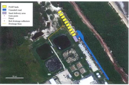
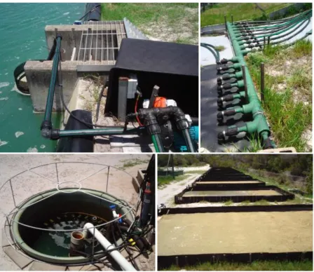
Figure 1 Aerial view of BIRC showing position of PASF development. ... 11

Figure 2 Construction of the PASF recirculation system at BIRC showing one of the pond water supply pumps (top left), the pond water mixing manifold (top right), the filtered-water collection sump (bottom left) and the completed PASF beds (bottom right). ... 13

Figure 3 Schematic diagram of the experimental integrated PASF recirculation system. ... 14

Figure 4 Schematic view of PASF prototype (all measurements in mm). ... 15

Figure 5 Harvest of prawns using traps (left) and live transport (right). ... 18

(6)

6 Figure 7 PASF bed showing short-circuit where water could routinely be released from the bed to allow sun drying (left) and the worm harvester (right). ... 22 Figure 8 Quadrat sampling from PASF beds showing worm holes/burrows and substrate structure with mottling of aerobic and anaerobic sediments. ... 24 Figure 9 Growth of black tiger prawns over 2 successive seasons (2013/14 and 2014/15) in 2 PASF-recirculated ponds. Mean (± se) weights achieved after stocking, relative to expected growth

(7)

7 Figure 26 Water pH levels in two recirculated prawn ponds (G1 and G2) and discharge from five deep and five shallow PASF beds (mean ± se) in Seasons 1 and 2. The licenced discharge minimum and maximum for BIRC are also provided. ... 45 Figure 27 Dissolved oxygen levels in two recirculated prawn ponds (G1 and G2) and discharge from five deep and five shallow PASF beds (mean ± se) in Seasons 1 and 2. The licenced discharge

(8)

8 Figure 44 Total phosphorus levels in discharge from four PASF beds (2 shallow and 2 deep) at

different times after the start of an artificial tide on two sample days in Season 2. ... 73

Figure 45 Total ammonia levels in discharge from four PASF beds (2 shallow and 2 deep) at different times after the start of an artificial tide on two sample days in Season 2. ... 74

Figure 46 Nitrite levels in discharge from four PASF beds (2 shallow and 2 deep) at different times after the start of an artificial tide on two sample days in Season 2. ... 74

Figure 47 Nitrate levels in discharge from four PASF beds (2 shallow and 2 deep) at different times after the start of an artificial tide on two sample days in Season 2. ... 75

Figure 48 Dissolved organic nitrogen levels in discharge from four PASF beds (2 shallow and 2 deep) at different times after the start of an artificial tide on two sample days in Season 2. ... 75

Figure 49 Dissolved organic phosphorus levels in discharge from four PASF beds (2 shallow and 2 deep) at different times after the start of an artificial tide on two sample days in Season 2. ... 76

Figure 50 Phosphate levels in discharge from four PASF beds (2 shallow and 2 deep) at different times after the start of an artificial tide on two sample days in Season 2. ... 76

Figure 51 Total sulphide levels in discharge from four PASF beds (2 shallow and 2 deep) at different times after the start of an artificial tide on two sample days in Season 2. ... 77

Figure 52 Total alkalinity levels in discharge from four PASF beds (2 shallow and 2 deep) at different times after the start of an artificial tide on two sample days in Season 2. ... 78

Figure 53 Estimated worm production from different juvenile stocking densities in PASF ... 92

Figure 54 PASF economic decision tool – Title page. ... 95

Figure 55 PASF economic decision tool – Bed Parameters worksheet (worked example). ... 96

Figure 56 PASF economic decision tool – Polychaete Production worksheet (worked example). ... 97

Figure 57 PASF economic decision tool – Post Production worksheet (worked example). ... 98

Figure 58 PASF economic decision tool – Labour worksheet (worked example). ... 99

Figure 59 PASF economic decision tool – Operating worksheet (worked example). ... 100

Figure 60 PASF economic decision tool – Capital worksheet (worked example). ... 101

Figure 61 PASF economic decision tool – Summary worksheet (worked example). ... 102

Figure 62 PASF economic decision tool – Risk Analysis worksheet (worked example). ... 103

Figure 63 PASF economic decision tool – Prawn Farm Benefits worksheet (worked example). ... 104

Figure 64 Pictures of outside (left) and inside (right) the covered broodstock pond (N1) at BIRC. .. 109

Figure 65 Mean (± se) weights of prawn broodstock grown in refilled production pond (G2) and covered pond (N1). ... 111

Figure 66 Pictures showing four different prawns sampled on 6 August 2014. ... 112

Figure 67 Harvested prawn broodstock being transferred to road transport tank. ... 113

Figure 68 Frequency of moulting and mortalities of broodstock following unilateral eyestalk ablation. ... 113

Figure 69 The experimental system showing tanks (left) and water supply from recirculation sump (right). ... 121

(9)

9

Executive summary

This study examined the physical and chemical properties of a novel, fully-recirculated prawn and polychaete production system that incorporated polychaete-assisted sand filters (PASF). The aims were to assess and demonstrate the potential of this system for industrialisation, and to provide optimisations for wastewater treatment by PASF. Two successive seasons were studied at

commercially-relevant scales in a prototype system constructed at the Bribie Island Research Centre in Southeast Queensland. The project produced over 5.4 tonnes of high quality black tiger prawns at rates up to 9.9 tonnes per hectare, with feed conversion of up to 1.1. Additionally, the project produced about 930 kg of high value polychaete biomass at rates up to 1.5 kg per square metre of PASF, with the worms feeding predominantly on waste nutrients. Importantly, this closed

production system demonstrated rapid growth of healthy prawns at commercially relevant production levels, using methods that appear feasible for application at large scale.

Deeper (23 cm) PASF beds provided similar but more reliable wastewater treatment efficacies compared with shallower (13 cm) beds, but did not demonstrate significantly greater polychaete productivity than (easier to harvest) shallow beds. The nutrient dynamics associated with seasonal and tidal operations of the system were studied in detail, providing technical and practical insights into how PASF could be optimised for the mitigation of nutrient discharge. The study also

highlighted some of the other important advantages of this integrated system, including low sludge production, no water discharge during the culture phase, high ecosystem health, good prospects for biosecurity controls, and the sustainable production of a fishery-limited resource (polychaetes) that may be essential for the expansion of prawn farming industries throughout the world.

Regarding nutrient discharge from this prototype mariculture system, when PASF was operating correctly it proved feasible to have no water (or nutrient) discharge during the entire prawn growing season. However, the final drain harvest and emptying of ponds that is necessary at the end of the prawn farming season released 58.4 kg ha-1 of nitrogen and 6 kg ha-1 of phosphorus (in Season 2). Whilst this is well below (i.e., one-third to one-half of) the current load-based licencing conditions for many prawn farms in Australia, the levels of nitrogen and chlorophyll a in the ponds remained higher than the more-stringent maximum limits at the Bribie Island study site. Zero-net-nutrient discharge was not achieved, but waste nutrients were low where 5.91 kg of nitrogen and 0.61 kg of phosphorus was discharged per tonne of prawns produced. This was from a system that deployed PASF at 14.4% of total ponded farm area which treated an average of 5.8% of pond water daily and did not use settlement ponds or other natural or artificial water remediation systems.

(10)

10

Introduction and background

Remediation and reuse of wastewater holds many benefits for intensive land-based aquaculture. On-farm water treatment and recirculation takes positive control of the most important element in an aquaculture operation: the water supply. With 100% recirculation, water and nutrient discharge during the growing season can be minimised, and reliance on natural waterways to replace water is reduced. In some places – for example, where water quality may be poor during or following heavy rainfall – water recirculation can offer much better surety of supply and quality than adjacent rivers and waterways. And for biosecurity, it can provide better protection from endemic diseases by greatly reducing a key vector for transmission (viz., inflow water).

In Australia, large-scale settlement ponds have provided water treatment services for prawn farms for many years (Preston et al., 2000). Upwards of 30% of farm ponded area is often committed to settlement ponds, and whilst this generally takes the place of otherwise productive pondage, farmers opt for this approach for nutrient mitigation because it is technically feasible and because it is accepted best practice. Alternative water treatment methods that use lower farm footprints and potentially create valuable commodities from waste nutrients have more recently been developed. Examples include sand beds and algal reactors by MBD Energy (2015) at the Pacific Reef Fisheries prawn farm in northern Queensland. Of similar utility and particular interest in this study are the polychaete-assisted sand filters (PASF) described by Palmer (2010), which have shown potential for water treatment (Palmer, 2008; 2011) and economical production of nutritious polychaete biomass (Palmer et al., 2014).

The intensification of prawn farming practices in Australia is also driving the investigation of better water treatment mechanisms. At the lower prawn stocking densities that were initially used in the 1980s and 1990s (e.g., 20 m-2) prawns were successfully farmed in ponds (typical area 0.5-1 ha) without any appreciable water exchange. This was made possible because the algal blooms that proliferate in these large-scale outdoor systems absorb dissolved nutrients and in turn provide an environment that facilitates high health and vigour in prawns. More recently however, farms in Australia are stocking ponds at higher rates (30-40 m-2, or higher), which invariably increases the levels of waste nutrients produced. As a result of these intensifications waste products need to be continually removed for ecosystem health. Licenced water discharge levels can also tend to be lower than operational levels in grow-out ponds, so farms need to more effectively treat their discharge. Prawn domestication is also seen as a high priority for farming practices in Australia. This is known to hold promising productivity gains through selection and specialised breeding practices (CSIRO, 2015), and also offer better surety of seed stock supplies and more control over disease within vertically integrated farms. Biosecure broodstock production systems will be needed to support such industrial endeavours in the future, as will increasing supplies of suitable polychaetes that are widely considered to be indispensable for prawn maturation diets (Harrison, 1990; Kawahigashi, 1998). Several operational imperatives will be necessary in these prawn broodstock culture systems, including well balanced nutrition, good water qualities, maintenance of adequate water

(11)

11 In considering PASF as an industrial option, there are several important considerations including: 1) water volumes able to be treated, 2) percentage of farm area needed, 3) capacity to adhere to licensed discharge levels, 4) suitability for water recirculation, 5) complexity for on-farm

management, 6) risk factors and surety of critical supplies, 7) investment and operational costs, 8) depreciation of equipment and long-term economic feasibility, 9) functional advantages the mechanism can provide.

The present study assesses PASF on these industrially relevant terms, and standardises the results for direct comparison with other potential methods. Since sand bed depth is an important aspect of PASF design, being likely to affect both water treatment efficacies and worm productivities, this was specifically investigated within a replicated prototype system and through robust water chemistry and seasonal system productivity assessments. Other factors investigated help to assess its industrial suitability and highlight novel aspects of this innovation for consideration by the mariculture

industry. The overall aim was to provide insight into how the PASF system can integrate with, and provide value for commercial prawn farming systems.

Materials and methods

PASF construction

In 2013, a 10-bed PASF system was constructed at the Bribie Island Research Centre (BIRC) funded by a Queensland Government Research Facilities Infrastructure grant. The system was designed to treat wastewater from any of the four larger (each 1600 m2) outdoor ponds on the site (Figure 1).

(12)

12 During the experimental period two of these ponds were stocked with prawns. Each PASF bed in the system was constructed to be operationally identical providing a 10-module configuration that could support replicated trials. System design provided similar operational conditions for each bed (e.g., surface areas, plumbing, inflow from ponds, head and suction pressures) and was based on the best prototype identified in previous work. Site preparation involved clearing vegetation, compaction and finishing the ground surface with a very slight slope (i.e., 50 mm in 10 m), and provision for heavy vehicle access (e.g., trucks carrying sand). Water supply and discharge installations involved pipe trenching for correct flows, and backfilling and re-levelling for smooth, flat ground surfaces.

After this, the PASF system was constructed. Pipes and materials most-commonly used in local rural activities were used, with considerations for their durability in the harsh (sun and seawater)

environment. High-density polyethylene (HDPE) pond liners (2 mm thickness) were used to form impervious bottoms and sides for the PASF beds. The corners of each bed were folded and welded to provide water-tight seals. Each bed was 9.3 m long and 5.8 m wide giving a surface area of 53.94 m2 (nominally 54 m2). This provided maximum width for beds constructed from rolls of plastic that were 7 m wide. Lengths of corrugated slotted ag-drain (50 mm diameter) were positioned across the width of beds at 900 mm centres to provide under-sand drainage, and this was connected to one main drainage line fashioned from 50 mm rural poly pipe. In the first season of the project, a heavy-duty geotextile sock (RTS grade) was used to cover the slotted drainage pipes. However in the second season, this was replaced with a slightly coarser (standard) grade to potentially help reduce the sock clogging that was apparent in Season 1.

PASF integrated design

Pumps were installed to draw water from inside a coarse (6 mm) screen next to the monk drain of two lined 1600 m2 ponds (Figure 2). These pumps were controlled with timers and synchronised to pump at specified times and for variable periods to deliver the desired daily volumes and flows. A manifold was installed to mix the water being supplied from the two ponds, so that each PASF bed was supplied with the same quality of wastewater. Flow meters (BIL DN 40 mm) measured the volumes of water supplied to each PASF bed, and daily adjustments to flows provided approximately similar total volumes (where possible) to each bed so that similar organic loading rates were applied. A 2,000 L sump with submersible pump and float switch was installed to collect all PASF-filtered water, and this was recirculated back to both ponds at equal rates.

Figure 3 provides a schematic diagram of the recirculated prawn/worm system. The total volume of the system (when the ponds were full) was 4.8 megalitres. The surface area ratio of PASF-treatment area (540 m2) to ponds (3200 m2) was 1 : 5.9. Not including the collection sump, water distribution pipes and manifold, the PASF beds used 14.4 % of total ponded farm area (ponds + PASF beds). The external standpipe arrangement (Figure 4) allowed the beds to be operated during wet weather1 by retaining a pool of pond water over the sand mass whilst potentially still filtering water.

1

(13)

13 Alternatively, during dry weather the drainage holes were used to continuously release filtered water from the PASF beds at controlled rates.

During dry weather the PASF beds were managed with three simulated tides each day, and

preferably so that the surfaces of beds could drain and dry in the sun each afternoon2. An example of the timing of pumps to achieve approximately 5% exchange with the ponds per day is given in Table 1 below. During wet operations, similar total daily pumping times (and volumes) were applied, but this was split into more pumping periods, 1) to provide more regular oxygenation of surface waters at night, and 2) to provide more regular supply for a more continuous percolation through the sand beds when head differentials were smaller.

Figure 2 Construction of the PASF recirculation system at BIRC showing one of the pond water supply pumps (top left), the pond water mixing manifold (top right), the filtered-water collection sump (bottom left) and the completed PASF beds (bottom right).

Internal overflow pipes installed on all beds were not generally used during normal operations so that all water pumped into the beds (according to flow meter readings) was treated via percolation

2

(14)

14 through the mass of sand. These overflows were a necessary design factor for use, 1) in case of oversupply of pond water, and 2) potentially during heavy rainfall when they would allow the lens of freshwater to be skimmed from the water surface.

Figure 3 Schematic diagram of the experimental integrated PASF recirculation system.

Prawn pond

G1

1600 m

2

x

1.5 m deep

= 2.4 mega-L

PASF beds – 54 m

2

x 10

Mixing manifold

Collection sump

(Not to scale)

Prawn pond

G2

1600 m

2

x

(15)

(16)

16 Table 1 Example of pond-water-supply pump timing for dry and wet weather operations of PASF.

Dry weather operations Wet weather operations

Pump on Pump off Pumping time Pump on Pump off Pumping time

4 pm 6 pm 2 hr 4 pm 5 pm 1 hr

10 pm 12 am 2 hr 8 pm 9 pm 1 hr

4 am 6 am 2 hr 12 am 1 am 1 hr

4 am 5 am 1 hr

8 am 9 am 1 hr

12 pm 1 pm 1 hr

Total daily pump time 6 hr Total daily pump time 6 hr

Filtration sand

Bulk sand purchased from a local sand mine (Southern Pacific Sands at Godwin Beach near Bribie Island) was used in the PASF system. The grade of sand used was GTS2000 (see Table 2) which had a hydraulic conductivity of 2,243 mm hr-1. This offered slightly higher percolation rates compared with a similar product that was successfully used in previous work (BMS2000 – 1,727 mm hr-1).

Table 2 Particle size distribution of sand used in the PASF beds.

SAMPLE Sieves (mm) 2.00 1.00 0.50 0.25 0.15 0.53 Pan

GTS2000 % Retained 0.8 6.4 27.3 60.0 5.0 0.2 0.4

After delivery to the site by single body trucks, a front-end loader tractor was used to initially load the sand into each bed. When loading the sand the bucket on the front of the tractor was used as a relative measure for sand volume. All deep beds (5) received 35 buckets and all shallow beds (5) received 22 buckets of sand. A small (5 tonne) excavator was used to roughly spread the sand, and this was finished to an even thickness and flat surface by hand rakes after drainage pipes were installed (via hand trenching with shovels). The finished average thickness after wetting and settling was 130 mm for shallow beds and 230 mm for deep beds.

Prawn pond operations

The two prawn culture ponds used in the study were an average of 1.5 m deep, had surface areas of 1600 m2, and therefore each pond held a maximum volume of 2.4 megalitres. They were fully lined and sealed with welded 1.5-mm high-density polyethylene plastic, which was replaced with new liner at the end of Season 1. One monk drain was positioned on one side of each pond, which provided a screened (6 mm) discharge/overflow point. All inflow seawater was screened with a

300-µm nylon sock. Pond filling began on 30/09/13 and 16/10/14 in Seasons 1 and 2, respectively. A standard pond fertilisation protocol (after Palmer et al., 2010) consisting of dolomite (300 kg ha-1 spread evenly over pond bottoms before fill) and N and P fertilisers3_{was applied during filling to}

3

(17)

17 encourage an algal bloom. Follow-up doses of inorganic fertilisers4 were then added to the ponds on a biweekly basis until Secchi depths5 reached 50 cm; this continued until about two weeks after stocking when enough nutrients to sustain the phytoplankton bloom was being added as formulated prawn feed. Blue dye (Aqua Blue – 2 satchels) was added to each pond when the initial algal bloom typically waned, and molasses was also added to each pond (1 L per day for 3-4 days) while the bloom was stabilising to help prevent the pH from climbing too high due to photosynthesis. Ponds were stocked with Penaeus monodon postlarvae nine days after filling began in Season 1 and seven days after filling began in Season 2. In Season 1, prawn ponds were stocked with

approximately 50,000 postlarvae (PL15) on 8 October 20136, and in Season 2 both ponds (G1 and G2) were stocked with 60,000 PL15 on 23 October 2014. This provided prawn stocking densities of about 31 m-2 in Season 1 and 38 m-2 in Season 2. In each year prawn seedstock were sourced from Truloff Prawn Farms at Alberton in southeast Queensland. They were progeny from wild broodstock captured in Joseph Bonaparte Gulf (14°06′S 128°50′E) in the Northern Territory.

Water quality measurements were undertaken in both ponds twice daily using a multi-probe meter (YSI Pro Plus) that simultaneously measured pH, dissolved oxygen, temperature and salinity. Measurements were taken in the morning (about 6 am) when dissolved oxygen levels were at their lowest (before any appreciable daily increase had occurred), and in the afternoon (about 3-4 pm) when pond pH values were near their maximum due to photosynthesis of the algal bloom.

Management of the prawn ponds was guided by the Australian Prawn Farming Manual (2006). This involved up to four feeds per day, with total daily feed amounts given by standardised percentages of total stock biomass; this was estimated from the average body weights of prawns multiplied by an assumed survival of those stocked (80% survival was assumed in both seasons). The feeding program was based on amounts recommended in the manual for subtropical regions (average daytime temperature <28°C). Ridley Aquafeed’s formulated prawn feeds were used in both years: the “Enhance” range was used in Season 1, and the “MR” range was used in Season 2. Feed trays (one per pond) were deployed each season from day 45 (45 days since stocking) to provide daily

measures of the prawns’ appetite and fine-tune feeding according to standard practices. Automatic belt feeders (four per pond) were also deployed at this time in association with airlifts to deliver and partially spread the mid-night ration.

Towards the end of each crop, and particularly in Season 2 when pond carrying capacities were particularly high and pH values started to decline, dolomite7_{(21 kg per week = 131 kg ha}-1_{) was}

applied to each pond to help stabilise pH and ensure adequate calcium and magnesium supplies for hard prawn shells. This was added by broadcasting the dry product onto the water surfaces around the entire periphery of the ponds. Also towards the end of each crop, when morning pH values

4

Monoammonium phosphate (9.5%): 1.2 kg ha-1; urea (47.5%): 6 kg ha-1; potassium nitrate (43%): 5.4 kg ha-1.

5

Secchi depth is a convenient measure of the turbidity of pond water.

6_{In Season 1 pond G2 was stocked with juveniles on the 15}th_{November 2013 after its PLs had alternatively}

been reared in a smaller pond for 6 weeks due to pond availability issues.

7

(18)

18 declined below 7, hydrated lime8 was also added to each pond (1-3 kg per day for 3-4 days in a row) by placing it in a 20-L bucket, mixing with pond water at high concentration in the bucket, and then partially submerging the bucket by suspending it in the flow of the aerator to produce a slow release of dissolving material. Care was taken during these later stages not to add too much lime due to low pH, so that afternoon pH values remained below 8.49; at this pH and with relatively high salinities and temperatures, total ammonia levels of over 2 ppm would yield increasingly dangerous levels of un-ionised ammonia (recommended to stay below 0.25 ppm by the Australian Prawn Farming Manual, 2006).

Both prawn culture ponds were continuously aerated with paddle wheels (2 hp; Chenta) and/or Force 7.2 submersible aspirators (1.5 hp; Acqua & Co.). Each pond was initially equipped with one operating paddlewheel. When morning dissolved oxygen (DO) levels started falling below 3 ppm (day 100), more aeration horsepower was added by installing an aspirator on the opposite side of each pond. Towards the end of Season 2 when high prawn carrying capacities were evident from low morning DO measurements, it was necessary to replace this aspirator with another paddlewheel (giving two paddlewheels per pond), which provided up to 25 hp of aeration ha-1. In Season 2 after almost all prawns had been harvested using traps, aeration was reduced to a minimum of one aspirator per pond.

Weekly prawn harvests (partial harvests from both ponds) commenced when they reached an average size of 30 g (on 19 February in 2014 and 2015). Up to four traps per pond were deployed and all prawns captured were transported live (Figure 5) to Truloff Prawn Farms at Alberton where they were processed using their standard methods. Quality assessments were made by comparing several physical attributes (e.g., apparent health and condition, shell hardness, and general appearance including colour and any superficial necrosis) with those of the farm’s own product.

Figure 5 Harvest of prawns using traps (left) and live transport (right).

As is typical of most prawn farming operations, no water exchange was applied to ponds for the first one to two months after fill. This approach generally conserves the nutrients added as fertilisers and allows a strong phytoplankton bloom to develop. Typically in the third month of culture, increasing

8

Hydrated lime: LIMIL from Sibelco, Aust.

(19)

19 amounts of pond water are discharged to waste, and this is normally replaced with new intake water so that phytoplankton densities and nutrients are regularly diluted (up to 10% exchange per day is often used where necessary). In the present study, instead of discharging this water to waste, it was treated by the PASF beds and fully recirculated back to the ponds. In Season 1, all wastewater was treated and recirculated up until the first prawn harvest (day 135 after stocking); after that,

wastewater was replaced with new intake water to ensure that no stock losses occurred10. However in Season 2, due to improvements made to the PASF system, all wastewater was treated by the PASF beds and recirculated back to the prawn culture ponds. This meant that in Season 2, no water was discharged from the integrated prawn/worm system until the final drain harvest of prawns (day 204 after stocking).

In Season 2, a prolonged period (50-51 d) between the last partial trap harvest (24/03/15) and final drain harvests (13 & 14/05/15) was implemented in an attempt to run the nutrient levels in pond waters down below BIRC’s discharge limits with PASF treatment. During this final water treatment period, no prawn feed was added to the ponds and aeration was reduced to one aspirator per pond.

PASF operations

All PASF beds were fully dried and screeded to provide a smooth sand surface before wetting with pond water. An even depth of sand was provided throughout each bed. Since the bottom liners had a 50 mm fall towards the underflow outlet (Figure 4), the surfaces of sand also had about 50 mm fall. This slight fall in the sand bed surface aids in maintaining a smooth progression of the advancing artificial tides, and also helps to prevent excess organic loading in depressions that inevitably form when the sand settles.

As a general rule, pond water supplies to the PASF beds in the past have been minimised before stocking polychaete seedstock, so that populations of potential predators (e.g., nematodes) that may exist in pond water are also minimised in the beds prior to stocking. After stocking polychaete seedstock, a three-day settling-in period has also been applied where wet-weather operations (see “PASF integrated design” Section above) maintains a pool of water above the sand beds, before normal dry-weather drain-down operations are implemented. Accordingly in the present study, pond water supplies to the PASF beds began just a few days prior to initially stocking the PASF beds with polychaetes each season, which was on 22/11/13 (46 days after stocking prawns into ponds in Season 1), and on 19/11/14 (28 days after stocking prawns into ponds in Season 2).

Polychaete seedstock used in the study were eighthgeneration (in 2013) or ninth generation (in 2014) domesticated Perinereis helleri supplied under contract by P&C Palmer Consolidated Pty Ltd. Nectochaete (three-day-old larvae) estimates were undertaken volumetrically in seawater and juvenile estimates were undertaken volumetrically in nursery sand. Nectochaetes were stocked into the pool of pond water over the PASF beds after a 50:50 dilution and a five-minute acclimation period. Juveniles were stocked into recently drained beds by shallow-planting small quantities (e.g., 400-500 mL) of nursery sand containing juveniles evenly across the entire beds’ surfaces, with pond water supplies resuming soon after.

10

(20)

20 Several approaches to seedstock supplies for the PASF beds were investigated in the study. In the first season higher densities and a more varied approach to stocking age was implemented (see below) to potentially demonstrate high production levels from various methods, and with a focus mainly on maximum polychaete biomass production. In the second season lower stocking densities were used with greater focus on live supplies and production of larger worms that are more suitable for bait markets.

Specifically in Season 1, 399,250 P. helleri nectochaetes were stocked into Beds 7, 8, 9, and 10 on the 25/11/13 and 26/11/13. This provided nectochaete stocking densities of 7,400 m-2 for these four beds. Beds 7 and 8 had been previously filled with water from Pond G1 containing a strong (50 cm Secchi depth) green chlorophyte bloom supporting a healthy copepod population; Beds 9 and 10 had alternatively been filled with water from Pond G2 containing a moderate (100 cm Secchi depth) brown diatom bloom supporting healthy populations of rotifers and copepods. To provide a pelagic environment for settlement of nectochaetes, beds were given three days of static operations (water pooled over sand beds with no water percolation) followed by three days of wet-weather

operational mode (pooled water over sand with percolation), before normal drain-down operations commenced. In addition to these nectochaetes, Beds 7, 8, 9 and 10 were also later stocked with a small number (20,000 per bed = 370 m-2) of two-month-old juveniles (on 24/01/14) when it appeared that the previously stocked nectochaetes had had low survival. The remaining six beds (Beds 1, 2, 3, 4, 5 and 6) were each stocked exclusively with 324,000 one-month-old juveniles on 28/11/13 and 29/11/13, giving stocking densities of 6,000 m-2.

In Season 2, all 10 beds were stocked with 108,000 one-month-old juvenile P. helleri on the 20/11/14 and 21/11/14, giving stocking densities of 2,000 m-2. Again, a minimised one-to-two day operational period was applied before stocking, and a three-to-four day settling-in period

(percolation with pooled water over the beds) was applied prior to commencement of normal drain-down operations.

After stocking and settling in periods, all beds were managed in exactly the same way regarding water volumes supplied and operational modes depending on the prevailing weather conditions (wet or dry weather operations – see “PASF integrated design” section above). Water supply rates to beds were managed and equalised on a daily basis by monitoring flow meter readings11.

Dry-weather operations were routinely applied unless the beds needed protection from rain with the wet weather operational mode. In Season 1, water treatment rates began with about 3% exchange of pond water per day, then after about one month rising gradually to a maximum of 9-10% exchange per day; whereas in Season 2, treatment rates began at a slightly higher rate with 4-5% exchange per day, rising to a maximum of 6-7% per day several weeks later (Figure 6). During the experimental periods the PASF beds treated an average of 6.6% of pond water daily in Season 1 and 5.8% in Season 2. Total volumes pumped from the ponds to the PASF beds each day were governed by how long the pumps operated each day. After the prawn ponds were drain harvested, clear water from one or two recently filled ponds (no fertilisers applied and no appreciable algal bloom) was used to continue this daily water supply to the PASF beds until they were also harvested.

11

(21)

21 One factor that was identified with potential to confound studies of nutrient concentrations flowing from the PASF beds was drainage rate. For example, higher drainage rates would tend to dilute dissolved nutrients being produced through the mineralisation of organic matter within the sand beds. To validly assess such differences between beds of different depths it was necessary to regularly equalise drainage rates during the experimental operations. This was made possible in the present work by the interchangeable size of drainage holes in the external standpipes (refer to Figure 4 above). Interchangeable standpipes with different sized holes ranging from 14 to 35 mm (diameters) were constructed for each bed, and removing the standpipe effectively provided the largest possible (50 mm) outlet. Daily observations on bed drain-down times guided the equalisation of bed drainage rates by changes to the size of drainage holes. As a general rule, if beds had not drained by noon each day, drainage hole sizes were increased to the next graduation, or if a bed appeared to be draining more rapidly than the rest, the hole size was reduced.

(22)

22 Beds that clogged to the point where their upper surfaces were not fully drying in the afternoon sun were short circuited by digging a hole in the sand close to the bottom outlet, disconnecting the first 19-mm drainage line from the main collection pipe and alternatively installing a 19-mm poly elbow (inside diameter of 16 mm) (Figure 7). This allowed a continuous slow (16 mm) discharge of

unfiltered water from above the sand mass. Whilst this was expected to reduce the efficacy of sand filtration, it still encouraged water to percolate down through the sand bed to filter some water and provide oxygen to worms within the mass of sand. This backup plan for clogged beds was developed towards the end of Season 1, but was standardised and routinely applied in Season 2 when the maximum outlet size (50 mm) could not provide sufficient water release for afternoon sun drying. Artificial feeding of the worms was initiated each season when the green-water supply from the ponds ceased. This was on the 3/04/14 in Season 1 and 15/05/15 in Season 2. Up to 400 g of prawn feed starter (Ridley Starter 1) was evenly spread on each bed when fully drained every one or two days. This was undertaken for two to four days per week and continued until the harvest of each bed began. Generally, no feeding was undertaken on weekends to allow uneaten feed to be fully

consumed, and no feeding was applied during wet weather operations when benthic algae tended to develop on the beds providing an alternative feed source for the worms.

Worms were harvested progressively from beds in Season 1 from 29/5/14 till 1/10/14, and in Season 2 from 1/04/15 till 14/10/15 using a modified dredge system that separated the worms from sand (Figure 7). Harvested worms were immediately placed on coarse sieves to remove sand and silt-laden mucus, then transferred to a 500 L raceway (6.5 m long x 30 cm wide x 25 cm deep) supplied with moderate aeration (6 x 30 mm airstones) and clean seawater exchange (10 L min-1) to allow purging of gut contents. The next day purged worms were weighed (after 10 s drip time in a fine net) to provide harvest weights from the previous day. Purged worms were then sorted so that only large worms (>0.6 g) were supplied to bait markets; large and small worms were supplied to prawn hatchery markets (live or frozen).

(23)

23 One half of each bed was harvested weekly in Season 1, with small worms and those large worms not sold as live product each week frozen in 250 g flat packs. Demand from live worm markets guided the amounts harvested in Season 2, where at times only one-quarter of a bed was harvested each week. Weights of worm biomass harvested from each bed were tallied, but importantly, comparisons of total harvests between beds were confounded by different culture periods; only quadrat samples (described below) provided valid worm production comparisons between treatments (i.e., between shallow and deep beds).

Experimental design

Sand bed depth was the main treatment investigated. It was studied both in terms of efficacies of water treatment and worm productivities. Two depths were each implemented in five beds during the initial loading of sand prior to Season 1. After wetting and settlement this provided five

replicates of either 230 mm (Beds 1, 3, 5, 7, 9 = deep beds) or 130 mm (Beds 2, 4, 6, 8, 10 = shallow beds). Using experience gained from several previous years of development, these depths were at the perceived extremes that could be practically managed and which would still offer a reasonable degree of water filtration. For example, overly deep sand beds present more difficulties in the harvest of worms using the current mechanical harvesting equipment, and overly shallow beds do not provide sufficient filtration media over drainage pipes. These two depths studied were on either side of the nominal 200-mm depth originally reported for PASF by Palmer (2010).

The maximum possible drainage rates of shallow and deep beds were experimentally compared at around the same stage in both seasons after a significant period of operation and at a time following the heaviest organic loading. In Season 1 this was undertaken on 25/02/14 after 94 days of

operation, and in Season 2 on 23/02/15 after 97 days of operation. These comparisons were made with the maximum hole size (50 mm – i.e., with stand pipes removed) in two ways: 1) using equal maximum head pressure with the same total depth of water (60 cm) over the discharge point (see “underflow pipe” in Figure 4) for all beds (note that over flow pipes were extended in shallow beds to facilitate this test), and 2) using the operational heads that the PASF system normally used, namely 43- or 53-cm depth over the discharge point for shallow or deep beds , respectively, which gave a 50 mm water depth over the highest surface of the sand beds at the highest part of the artificial tide.

(24)

24 Figure 8 Quadrat sampling from PASF beds showing worm holes/burrows and substrate structure with mottling of aerobic and anaerobic sediments.

To assess prawn growth, weekly samples of 10-12 prawns were randomly taken from each pond and individually weighed. Initially these were captured with fine nets or taken from feed trays, but when prawns reached an average size of 8-9 g a cast net was used to obtain each sample. Mean sizes in each pond were compared with the growth expected under sub-tropical conditions as provided by feeding charts in the Australian Prawn Farming Manual (2006). Total prawn production was assessed by adding partial harvest amounts with final drain harvest amounts and weights of progressive size check samples.

The replacement of pond liners at BIRC between Seasons 1 and 2 allowed some other interesting assessments (e.g., accumulation of pond sludge and barnacle growth) that otherwise would have been more difficult in previously used ponds. To estimate the volumes, solids and organic contents of settled materials in each pond, the circular sludge piles that accumulated on the middle bottom of each pond in Season 2 were sampled and measured one or two days after draining Pond G2 or G1, respectively. An approximate diameter and four evenly-spaced depths across the radii of the piles provided a rudimentary way of estimating volumes, using the CAD computer graphics program (see Results) which converted the piles to flat circular discs and calculated volumes as a cylinders. Three samples (300 mL) of sludge were taken across radii of the piles in each pond on the same days that volume estimates were made. These were submitted to Unitywater Laboratories and ALS

(25)

25 Densities of barnacles on the walls of each pond were also assessed after draining ponds in Season 2. This was undertaken by counting the number of barnacles within 12 stratified rectangular quadrats for each pond. A frame fashioned from aluminium angle was used to standardise quadrat samples at 50 mm wide and 1500 mm long (0.075 m2). Quadrats were vertically arranged from the water level down, with one sample positioned in each pond corner (4 per pond), and two samples (10 m from corners) on each wall.

Water quality and nutrient measurements

To facilitate routine prawn pond management decisions, twice-daily water quality measurements of dissolved oxygen (DO), pH, temperature and salinity were undertaken by submerging a multi-probe system (YSI Pro Plus) in one corner of each pond. Daily measurements were generally timed to coincide with the lowest daily DO levels (about 6 am) and the highest daily pH levels (around 4 pm). These water qualities were also studied in the PASF discharge through weekly or fortnightly

measurements (around 8 am) taken by submerging the probe inside the discharge pipe of each PASF bed.

Notably in Season 1, pond availability at BIRC prevented the study of two identical ponds prior to the start of water recirculation through the PASF beds. As a proxy for pond G2 during this time, data collected from the smaller covered nursery pond (N1) holding the prawn juveniles (that were later transferred to pond G2) is presented. This caused several water quality differences that are apparent in the data between the ponds before the prawns were transferred on 15/11/13, including higher water temperatures and different Secchi depths.

To study nutrients and other water chemistry, weekly or fortnightly water samples were taken from the discharge of each bed and from the mid-water column near the pump intakes in each pond. Samples from PASF beds reflected the same water being recirculated back to the ponds. This

seasonal sampling was routinely undertaken in the mornings during mid-tidal flows, which tended to occur between 7 and 8 am. Water samples were immediately placed on ice and submitted to Unitywater Laboratories for NATA-accredited analyses on the same day that samples were collected. Parameters studied included total suspended solids (TSS), turbidity, chlorophyll a, total nitrogen (TN), total ammonia (TAN), nitrite, nitrate, dissolved organic nitrogen (DON), total phosphorus (TP), phosphate, dissolved organic phosphorus (DOP), total sulphide and total alkalinity12.

In Season 1, water nutrient sampling was suspended after the short circuiting of beds (that was necessary due to sand bed clogging) because this confounded the PASF filtration effect by allowing water to track past the sand filtration process. However in Season 2 water quality studies extended through a bed-clogging (e.g., overload) event, and then well past the last trap-harvest of prawns to study the potential for PASF to recover from clogging and to continue operating. This later interest in the ability of PASF to reduce nutrient levels in the ponds after pond feeding had ceased, when prawn stocks were at a minimum, relates to the disposal of pond water with the drain harvest. The effect of wet-weather operational mode on PASF efficacies was studied on two occasions when scheduled sample days coincided with wet weather. This occurred on 7/01/14 in Season 1 and on 12/02/15 in Season 2. All other water samples were taken during routine dry-weather operations.

(26)

26 In addition to these routine weekly/fortnightly water samples, two time-series experiments were performed in Season 2 as the organic loading built to a maximum (i.e., on 19/01/15 and 16/02/15). This was undertaken to evaluate the changes in nitrogen, phosphorus and dissolved nutrients present at different stages of the tidal outflow from PASF. The experiments simulated normal afternoon tidal flows with an inflow duration of 2.5 hr, with samples taken as pond water slowly covered the sand beds and then began to recede (e.g., approx. 10% covered at 5 min, 50% at 15 min, 75% at 30 min, 100% at 60 min, 3-4 cm deep over highest part of bed at 120 min, and 1-2 cm deep at 240 min). They involved samples from two shallow and two deep beds at 5, 15, 30, 60, 120 and 240 min after the inflow began at 4 pm. Beds 5 and 9 (deep) and 8 and 10 (shallow) were studied on 19/01/15, and beds 7 and 9 (deep) and 8 and 10 (shallow) were studied on 16/02/15. Parameters measured included TN, TP, nitrite, nitrate, TAN, phosphate, DOP, DON, total sulphide and total alkalinity.

Statistical analyses

In cases where laboratory results were lower than their minimum detection limits, arbitrary levels of half their detection limit were assigned in order to avoid un-natural skewness in the data towards zero. Results were analysed with GenStat (2015) using one- or two-way ANOVA and LSD pairwise comparison of means. The time-series nature of the seasonal and tidal water quality data was taken into account by an analysis of variance of repeated measures (Rowell and Walters 1976), via the AREPMEASURES procedure of GenStat (2015). This forms an approximate split-plot analysis of variance (split for time). The Greenhouse-Geisser epsilon estimates the degree of temporal autocorrelation, and adjusts the probability levels for this.

Results and discussion

Prawn production

Prawn production during the study was very successful in the PASF-recirculated system. Compared with the “Sub-tropical Growth” projections provided in the Australian Prawn Farming Manual (2006), above-average prawn growth was achieved in both seasons (Figure 9). Growth was particularly good in Season 2, but this may have been due to several factors unrelated to the recirculation of

wastewater, including higher prevailing temperatures (see the section below on Seasonal water qualities) and the change to the more-advanced MR range of feeds offered by Ridley Aquafeeds. Table 3 provides a summary of other prawn production statistics for the two seasons. In Season 1, higher survival was apparent in Pond G1 than in Pond G2, which was very likely due to the need to grow and transfer the prawns between two ponds during the grow-out cycle. This also likely caused the lower prawn production and higher feed conversion ratio in pond G2.

(27)

27 from that pond; sufficient natural feed (including detritus and pond biota) may have allowed the remaining lowest-density prawns to maintain a reasonable growth trajectory despite the lack of a high-protein pellet diet.

Figure 9 Growth of black tiger prawns over 2 successive seasons (2013/14 and 2014/15) in 2 PASF-recirculated ponds. Mean (± se) weights achieved after stocking, relative to expected growth according to the Australian Prawn Farming Manual (2006).

Prawn quality was assessed as outstanding in the study. In both seasons harvested prawns that were supplied live to one of the major prawn producing companies in Australia were visually no different from that farm’s own produce. Being supplied live to the farmers meant that there was no

deterioration of the product due to chilling or storage prior to cooking. Factors taken into consideration were overall size, evenness of size, colour, and general health. There was no

(28)

28 transport time. In the farm’s view the prawns were as good as their own farm produce, and they were processed through their processing plant in a similar manner to their own product.

Table 3 Prawn production statistics for Seasons 1 and 2.

Parameter

Season 1 2013/14 Season 2 2014/15 Pond

G1

Pond N1/G2

Pond G1

Pond G2

Number of postlarvae (PL15) stocked 50,000 50,000 60,000 60,000

Stocking density (PLs m-2) 31.3 31.3 37.5 37.5

Calculated* survival (%) 67.3 61.6 71.1 68.9

Total harvest (kg pond-1) 1164.8 1095.1 1579.9 1580.5

Total harvest (tonnes ha-1) 7.28 6.84 9.87 9.88

Age** at first trap harvest (d) 135 135 120 120

Mean prawn weight at first trap harvest (g) 26.9a 29.1a 27.8b 30.8b

Age** at final drain harvest (d) 165 163 204 205

Mean prawn weight at drain harvest (g) 42.7 40.5a 45.1 54.9 Harvested amounts at drain harvest (kg) 265.2 191.4 38 21.6

Feed conversion ratio 1.3 1.32 1.12 1.14

*Based on weights harvested divided by previous size estimates. **Number of days after stocking as PL15.

ab_{Estimates made 2 days}a_{or 1 day}b_{before harvest.}

Sludge production

The sludge piles that accumulated in each pond in Season 2 (Figure 10) had approximate volumes of 5.47 m3 in pond G1 and 7.96 m3 in pond G2 (see Figure 11 for volume calculations). Levels of

moisture, volatile solids and macronutrients of the sludge piles (Table 4) were not significantly different between the two ponds (P>0.05).

Table 5 provides some mass balance calculations for the estimated volumes of sludge in each pond at the end of Season 2, including wet weight estimates, dry weight calculations, and calculated total nitrogen and total phosphorus.

(29)

29 Figure 11 Sludge volume estimates given by CAD program output on cross-sectional (XS) area and standard cylinder volume calculations.

Table 4 Contents (mean ± se, n = 3) of accumulated sludge in ponds after the drain harvest in Season 2. Within rows, means with similar letters are not significantly different (P > 0.05).

Parameter Pond G1 Pond G2

Moisture (%)* 90 ± 1.54a 91.6 ± 0.64a

Total volatile solids (% total solids)** 32.7 ± 1.92a 34.9 ± 0.49a Total nitrogen as N in dry matter (g kg-1)* 213.2 ± 60.43a 259.2 ± 36.76a Total phosphorus as P in dry matter (g kg-1)* 111.4 ± 39.72a 180.3 ± 7.03a

*Tested by ALS Laboratories; **Tested by Unitywater Laboratories

Table 5 Mass balance calculations using mean values provided in Table 4 for sludge left in the middle of each pond after the drain harvest in Season 2.

Parameter Pond G1 Pond G2

Average weight (mean ± se, n = 3) of wet sludge (kg L-1) 1.048 ± 0.007 1.065 ± 0.021 Wet weight of sludge (tonnes) (= volume x average weight) 5.732 8.482 Wet weight of sludge (tonnes ha-1) (x 6.25 multiplier) 35.825 53.01 Dry weight of sludge (tonnes ha-1) (minus moisture) 3.583 4.983

Dry weight of sludge (kg pond-1) 573.28 797.28

Total nitrogen in sludge (kg ha-1) 763.9 1,291.6

Total nitrogen in sludge (kg pond-1) 122.2 206.7

Total phosphorus in sludge (kg ha-1) 399.1 898.4

(30)

30 Whilst these data were considered somewhat imprecise13, they do provide a standardised way to evaluate and compare sludge piles in future work with PASF and in other prawn farming systems. For example, Robertson et al. (2003) compared the traditional flow-through prawn farming model with a recirculated design using vertical artificial substrate within a settlement pond. Although our methods of calculating sludge volumes were different from those used by Robertson et al., the amounts of sludge that accumulated in ponds in the present study were much lower. In Robertson et al., dry weight sludge volumes were estimated to be 96.9 tonnes ha-1 for recirculated ponds and 47.38 tonnes ha-1 for flow-through ponds, which are both many fold higher than estimates made in the present study (less than 5 tonne ha-1: Table 5).

Robertson et al. (2003) considered methods of sludge removal during the cropping cycle for their recirculated approach. In the present study, by contrast, all sludge was left in the pond at the end of Season 2, and spread around the bottom of the pond before refilling (Figure 12) so that it could usefully contribute to nutrients needed for bloom development in the next crop. About 33% of the solids which accumulated in the centre of ponds in Season 2 was organic matter (volatile solids), and this is also quite low compared with previous key nutrient-budget studies for flow-through prawn farming systems with 5-10% water exchange per day (e.g., Funge-Smith and Briggs, 1998: 63% organic matter).

Figure 12 Pond G2 prior to refilling after Season 2. Sludge was allowed to dry and crack in the sun and was then spread away from the centre of the pond (as shown) to provide nutrients for the next pond bloom.

This is an important finding, since sludge production and its removal from ponds and disposal can be significant problems for farmers. Standard practice is to allow it to de-water after the drain harvest and dry until it cracks in the sun before physical removal with heavy machinery. It is generally placed into land fill sites that are well away from natural water flows. However, this accumulation of sludge is greatly increased when the suspended solids contents of intake waters at flow-through farms are

(31)

31 continually added to ponds with regular (daily) water exchanges. On some farms this can be

excessive requiring removal each year.

Essentially, prawn farmers using flow-through systems are providing two settlement zones for suspended solids that are captured from adjacent natural waters; namely, the centres of their prawn grow-out ponds, and (in Australia) their dedicated settlement ponds, which capture further

settleable solids prior to release of their wastewater. Many farmers have lined the sides of their grow-out ponds with HDPE plastic to minimise the erosion of pond embankments caused by circulating pond waters, since bank erosion can contribute significantly to settleable solids in the farming system (Burford et al., 1998). Full recirculation eliminates these regular additions of silts (with exchange water) to the farming system. And, in turn, PASF appears to further reduce this accumulation of settled solids and organic matter sludge of prawn ponds, probably because of sediment capture in the worm beds.

Worm production

A total of 570 kg of worm biomass was harvested in Season 1. This provided a production average of 1.056 kg m-2 over a 307-day culture period. This total was a combination of the smaller controlled-harvest samples taken during the culture phase and larger operational partial controlled-harvests. The total amount of supplemental feed added to the worm beds in Season 1 was 263 kg providing a 1:2.17 feed-to-worm conversion ratio. This artificial-feed conversion ratio does not take into account the algae-based feed and includes the considerable growth of worms during the water filtration phase of the experiment during which no supplemental feed was added (up to day 126).

In Season 2, a total of 353 kg of worm biomass was harvested providing a production average of 0.654 kg m-2 over a 328-day culture period. Again this included both controlled samples (to estimate survival and compare production across treatments) and operational harvests14. Most of this

polychaete biomass was sold at critical times each season into fishing bait and prawn broodstock feed markets, either as live or frozen products. Supplemental feed totalling 92 kg was used in Season 2 (from day 177), which was much less than in Season 1 because of the longer availability of green water which alternatively fed the worms for longer in Season 2. This gave an artificial-feed

conversion of 1:3.85. Pictures of live harvested worms in the storage raceway and frozen flat packs of worms are provided in Figure 13, and the harvested amounts and relative dates of final harvests for each bed with their respective ages at final harvest are provided in Table 6.

Operational worm harvests began on 29/05/14, 184 days after stocking in Season 1, but earlier in the second season (1/04/15) at 134 days after stocking. This earlier first harvest date in Season 2 was stimulated by market interest and larger prevailing worm sizes due to the relatively low stocking density. Although age (or culture period) had a strong influence on quantities harvested, which gradually increased during each season, this was unlikely to have been the main reason for the higher production in Season 1. This was presumably more due to the lower stocking densities applied in Season 2 (2,000 m-2), compared with Season 1 (>6,000 m-2). Although compromised by

14_{Progressive harvesting prevented the use of final harvest figures for formal statistical analyses of the effects}

(32)

32 different ages and culture periods, in Season 1 higher mean (± se) total harvests were obtained from PASF beds that were stocked with one-month-old juveniles (1.24 ± 0.07 kg m-2) than beds that were predominantly stocked with nectochaetes (0.78 ± 0.14 kg m-2). The highest production in both seasons was a deep bed (Bed 3) in Season 1 which produced over 79 kg (1.474 kg m-2) harvested 293 days after stocking 6,000 m-2 one-month-old juveniles.

Figure 13 Harvested live worms in raceway (left) and frozen flat packs of worms (right).

Harvest strategies each season took into account the densities and sizes of worms that were apparent from the controlled quadrat sampling. Beds with more smaller worms were harvested last because they were assumed to have more potential to grow to larger sizes for higher overall polychaete biomass production. Conversely, beds that appeared to have lower densities and larger worms were harvested first because they were assumed to have reached closer to their production potential, and because they could supply markets wanting larger worms earlier. Of course,

sequential harvests were necessary to some degree because all beds could not be harvested at once, and as discussed previously the commercial orientation of this strategy prevented total harvest data being used in thorough statistical analyses. However, this is partially circumvented by using daily growth rates which took into account their relative ages (see last column in Table 6). Deep beds produced an average (± se) of 4.33 ± 0.25 and 2.47 ± 0.1 g m-2 d-1, and shallow beds produced an average of 3.82 ± 0.44 and 2.8 ± 0.2 g m-2 d-1, respectively in Seasons 1 and 2. In most cases it appeared that the longer the worms grew in the beds, the greater the amounts of polychaete biomass that could be harvested; but these data also show that daily growth rates generally increased during each season, which is likely due to the onset of summer and warmer waters for faster metabolism and growth later in each season, coupled with the exponential growth (as is seen in other animals) that is facilitated by increasing feed intake as the they grow to larger sizes.

(33)

33 bed depth. However, much higher (P<0.05) densities did prevail in beds stocked with one-month-old juveniles, compared with beds predominantly stocked with worm larvae (nectochaetes) (Figure 14). Table 6 Worm harvest weights for polychaete-assisted sand filters in Seasons 1 (2014, grey) and 2 (2015, blue).

Sequence and dates of final

harvests

PASF bed Harvest total

(kg)

Harvest total (kg m-2)

Age after stocking* (d)

Polychaete biomass production

(g m-2 d-1)

4/06/2014 8 22.9 0.425 191 2.22

18/06/2014 7 43.6 0.808 205 3.94

2/07/2014 9 42.6 0.788 219 3.60

15/07/2014 10 58.8 1.088 232 4.69

8/08/2014 6 58.5 1.083 253 4.28

20/08/2014 5 64.8 1.2 265 4.53

3/09/2014 4 54 0.999 279 3.58

17/09/2014 3 79.6 1.474 293 5.03

25/09/2014 1 73.8 1.368 301 4.54

1/10/2014 2 71.7 1.328 307 4.33

8/04/2015 9 14.8 0.274 138 1.98

6/05/2015 10 24.9 0.461 166 2.78

27/05/2015 8 28.3 0.523 187 2.80

1/07/2015 6 30.3 0.56 222 2.52

5/08/2015 4 48.9 0.905 258 3.51

19/08/2015 2 34.8 0.644 272 2.37

1/09/2015 7 50.8 0.94 284 3.31

16/09/2015 5 38.2 0.708 300 2.36

7/10/15 1 42.5 0.787 321 2.45

14/10/15 3 39.5 0.732 328 2.23

*Time from first stocking to date of last harvest.

(34)

34 Taking into consideration the total number of larvae and/or juveniles that were stocked in Season 1, survival was also not significantly affected by sample date or sand bed depth (Figure 15), but again, one-month-old juveniles provided much higher (P<0.05) mean rates of survival (32.2 ± 3.62 %) compared with larvae (9.7 ± 1.04 %). Furthermore, the mean (± se, n=2) survival of larvae stocked into PASF beds that had an underlying base of chlorophytes and copepods from one source pond (as estimated on the second sample date of Season 2) was 8.6 ± 1.75 %, which is similar to the result of 10.8 ± 1.08 % given in two different beds supplied with an underlying base of diatoms and rotifers from the other pond. These subtle changes in the ecology of PASF beds did not seem to affect the survival of larvae.

Figure 15 Mean (± se) survival of worms sampled from beds before (Sample 1) and after (Sample 2) supplemental feeding for seven weeks in Season 1.

Worm sizes (Figure 16) and worm biomass production (Figure 17) in Season 1 were again not significantly affected by sand bed depth, but both worm size and worm biomass were much higher (P<0.001) in older worms (in Sample 2). Worm sizes were larger (P<0.05) in PASF beds stocked predominantly with larvae, and we speculate that this is due to the lower densities and lesser competition that prevailed. Worm biomass was higher (P<0.05) for beds stocked with one-month-old juveniles.

(35)

35 Figure 16 Mean (± se) size of worms sampled from beds before (Sample 1) and after (Sample 2) supplemental feeding for seven weeks in Season 1.

Figure 17 Mean (± se) biomass of worms sampled from beds before (Sample 1) and after (Sample 2) supplemental feeding for seven weeks in Season 1.