Finite Element Modeling of A phenomenological Constitutive Model for Super-elastic Shape Memory Alloy and its Application for Preload Process Analysis of Bolted Joint
Xiangjun Jiang1; Huang Jin1; Yongkun Wang1*; Fengqun Pan1; Baotong Li 2; and Peng Hao 3
1 Key Laboratory of Electronic Equipment Structural Design, Xidian University, Xi'an, Shaanxi, 710071, P.R.C. E-mail:
2 State Key Laboratory for Manufacturing System, Xi’an Jiaotong University, Xi'an, Shaanxi, 710049, P.R.C. E-mail:
3 State Key Laboratory of Structural Analysis for Industrial Equipment, Dalian University of Technology, Dalian,
Liaoning, 116023, P.R.C. E-mail: [email protected]
Abstract
A phenomenological constitutive model is developed to describe the uniaxial transformation
ratcheting behaviors of super–elastic shape memory alloy (SMA) by employing a cosine–type
phase transformation equation with the initial martensite evolution coefficient that can
capture the feature of the predictive residual martensite accumulation evolution and the nonlinear
hysteresis loop on a finite element (FE) analysis framework. The effect of the applied loading
level on transformation ratcheting are considered in the proposed model. The evolutions of
transformation ratcheting and transformation stresses are constructed as the function of the
accumulated residual martensite volume fraction. The FE implementation of the proposed model
is carried out for the numerical analysis of transformation ratcheting of the SMA bar element. The
integration algorithm and the expression of consistent tangent modulus are deduced in a new form
for the forward and reverse transformation. The numerical results are compared with those of
existing model and the experimental results to show the validity of the proposed model and its FE
implementation in transformation ratcheting. Finally, a FE modeling is established for a repeated
preload analysis of SMA bolted joint
keywords: SMAs; Super-elasticity; FE implementation; Phase transformation ratcheting; Preload process analysis of bolt
1. Introduction
SMA has been widely applied in MEMS, actuators, biomedical devices, organ transplantation,
transportation, aerospace and civil engineering due to its well-known super–elasticity, shape
memory effect, excellent biocompatibility and wear resistance [1-3]. In the last two decades, with
the deeper understanding of thermo–mechanical coupling behavior of SMA, more and more
scholars pay attention to the response of thermo–mechanical coupling behavior of the alloy
undergoing cyclic loading. The cyclic deformation behavior of SMA, as described in earlier
research, was followed with interested by the research group led by Miyazaki [4–5]. The group's
research concluded that, the residual irrecoverable deformation of SMA would increase gradually
with the increase of cycle times under the mechanical loading cycles. The phase transformation
stress would also decrease with the increase of cycle numbers. Strnadel et al. [6-7] had studied the
effect of alloy elements and components on mechanical cyclic deformation behavior of
super–elastic NiTi alloy by experiments, and revealed the inhibition effect of high nickel content
on cyclic residual deformation. Nemat–Nasser had also observed the deformation features of
super–elastic NiTi alloy under cyclic loadings by experiments [8]. It was revealed that the
increment of residual martensite strain and the dissipation energy decreases with the increase of
cycle numbers, and tend to be stable following several cycles.
The super–elasticity of NiTi SMA gradually deteriorates during the process of cyclic
deformation. This phenomenon could mainly be expressed as four aspects: the residual
martensite strain accumulation, the gradual decrease of transformation stresses, the gradual change
of phase transformation modulus, and the gradual decrease of dissipation energy with the cyclic
loadings [5, 9-13]. The researches done by [14-20] show that the mechanical behavior of the alloy
is strongly dependent on the loading rate. The non–monotonic relationship can be found between
the dissipation energy and the loading rate. The mechanical dissipation and the latent heat of phase
transformation cause the heat generation of the alloy. Kan et al. [21] had also studied
experimentally the cyclic deformation behavior of the untrained super–elastic NiTi SMA at
different loading rates. The results show that all of the phase transformation modulus, the starting
stress of martensitic transformation, the hysteresis loop and the residual strain of NiTi SMA are
strongly dependent on the loading rate.
constitutive models had been built by different scholars [22–25] to describe the
thermo–mechanical coupling deformation characteristics of SMA. As a further work, the FE
implementation of the proposed model was to be carried out to calculate an accurate stress-strain
responses for SMA-based devices. In the generalized plasticity frame, the return-mapping
algorithm was utilized for the analysis of super-elastic NiTi alloy. [26, 27]. However, it was not
yet possible to describe the deterioration of super–elasticity and shape memory effect of untrained
materials during cyclic deformation. In view of the shortcomings of the above work, some
scholars had further extended the above constitutive model. Based on the existing experimental
observations with cyclic deformation, the corresponding cyclic constitutive model were
established by Lagoudas and Auricchio [28] to describe the accumulation of interfacial defects and
residual martensite in cyclic deformation. Though the Lagoudas’s model shows a good capability
in the prediction of the nonlinear hysteresis loop shape with a lot of material parameters, that
model can only give a reasonable description for the cyclic deformation characteristic of a specific
loading conditions, instead of predicting the dependence of that one on the applied loading level.
Kan and Kang [29-30] made a further expansion of the cyclic constitutive model based on the
experimental observation by Kang [31] that is able to reasonably describe the applied loading
level related to super–elastic deterioration phenomenon. Furthermore, the Kan-Kang's model
accounts for the asymmetric effect of tension and compression of the material on the phase
transformation ratcheting behavior and the effect of applied loading level with just
a small number of material parameters. Nevertheless, the linear phase transformation hardening
rule employed by Kan-Kang's model cannot predict the nonlinear hysteresis loop shape well.
This paper thus develops a phenomenological constitutive model to describe the uniaxial
transformation ratcheting behaviors of super–elastic SMA. A cosine–type phase transformation
equation with the initial martensite evolution coefficient that can capture the feature of the
predictive residual martensite accumulation evolution and the nonlinear hysteresis loop is
employed in the proposed model on a FE analysis framework. The return-mapping algorithm and
the consistent tangent modulus are deduced in a new form for the phase transformation. The
validity of the proposed model and its FEimplementation in transformation ratcheting is finally
examined by comparison between the proposed model and the existing model and experimental
bolted joint.
2 Constitutive modeling for NiTi SMA under cyclic loading
In the last one decade, many researchers focused on the constitutive modeling to describe the
cyclic deformation of NiTi SMA. The phenomenological constitutive model shows good candidate
to be integrated into the structure computational methods, such as FE method, to predict the cyclic
deformation of SMA structure. However, these models with FE implementation seem to be
difficult to analyze efficiently the complex structure due to relatively low computation efficiency
and nonlinearity.
Therefore, in this work, an one–dimensional constitutive model for phase transformation
ratcheting of super–elastic SMA is proposed based on the Brinson–model, and then implemented
into FE model of one–dimensional bar element to describe the cyclic deformation of some
mechanical structures, such as SMA bolt joint, SMA washer, and so on.
2.1 Constitutive equation and internal variables
In the proposed model, the total strain
can be decomposed into an elastic strain tensor
eand an inelastic strain tensor
in with infinitesimal strain assumption.e in
(1)The residual deformation of SMA under cyclic loadings is considered to be attributed to the
residual martensite deformation due to the phase transformation ratcheting. In order to
characterize this deformation mechanisms, there are two internal variables are introduced here in
Helmoltz free energy, which is assumed to be additively decomposed into elastic and inelastic
parts, as follow:
)
,
,
(
)
,
,
,
(
inT
inT
e
ε
ε
ψ
ψ
ψ
(2)The internal variable
as the martensite volume fraction depicts the stress–inducedmartensite phase transformation, and is constrained by 0≤
≤1.
characterizes theaccumulative martensite transformation, including the accumulated martensite volume fraction
c
.:
(
in, , , )
( , , ) 0
e
T
in
T
σ ε ψ ε ε
ψ
(3)where
: (
)
: (
)
(
)
in in
e in
ψ
ψ
σ ε ε
ε ε
ε ε
(4a):
:
:
:
in c
c
ψ
ψ
ψ
ψ
ψ
(4b)The incomplete phase transformation between martensite and austenite could be observed
during the cyclic phase transformation [29–31]. Furthermore, the amount of residual martensite
would increase with the increasing number of loading cycles. Therefore, the total
induced–martensite volume fraction
that represents the progressive increase of residualmartensite strain is set as internal variable and divided into two parts, i.e., reversible martensite
volume fraction
r and irreversible residual one
ir.r ir
(5)According to the experimental observations, the phase transformation deformation evolves
with the increasing number of loading cycles, and reaches a stable value after a certain cycle
[29–31]. In order to account these evolution process, the internal variable
c is picked as theaccumulated martensite volume fraction
c that represents the evolution process of somevariables and material parameters with the increasing number of cycles, and is written by
0
|
( ) |
t
c r
d
(6)where, t is a kinematic time.
Based on the frame of generalized plasticity, the total inelastic strain
in in Eq. (1) equals tothe transformation strain
tr from stress–induced martensite phase and its reverse.in tr
(7) The SMA constitutive model used here is based on a model originally formulated by [22–23],which is a phenomenological macro–scale one–dimensional constitutive model and can be written
0
( )
( )
0 0Θ(
0)
( )
( )
0 0s s
E
E
T T
(8)where
E
s is the Young’s modulus,
is the transformation coefficient,Θ
is the thermalelastic coefficient;
T
is the temperature. The subscript ‘0’ indicates the initial values. Young’smodulus
E
s and transformation coefficient
are the function of the martensite volumefraction
, which are given as( )
(
)
s
A M A
E
E
E
E
(9a)( )
s( )
L
E
(9b)It is assumed that the equivalent transformation strain and the recoverable martensite volume
fraction shows proportional relationship (irreversible martensitic transformation does not
participate in the transformation process). Then, the following relationship can be obtained
tr
L
(10)Eq. (5) illustrates that the total induced–martensite volume fraction
consists of reversiblemartensite volume fraction
r and irreversible residual one
ir. Since the irreversiblemartensitic transformation does not take part in the phase transformation process, the stress is only
the function of reversible martensite volume fraction, which is irrelevant to the residual martensite
volume fraction in the phase transformation. The expression forms of
r are as follows:(i) Transformation to martensite phase
if
T
M
S and
scr
C T M
M(
s)
crf
C T M
M(
s)
:1
1
cos
[
(
)]
2
2
ir ir
f f
r M A cr M A
f M S
cr cr
A M s f
C T M
(11) (ii) Transformation to austenite phaseif
T
A
S andC T
A(
A
f)
C T
A(
A
s)
:cos[ (
)] 1
2
r ir
f M A
r A M
A s
M A A
a T A
C
(12)where, cr s
M
C
are slope for the relation between critical transformation stress and temperature,A
s andf
A
are starting and finishing temperature of austenite transformation,M
s andM
f arestarting and finishing temperature of martensite transformation, rf
A M
is the volume fraction of
martensite transformation at the end of transformation to martensite phase, irf
M A
is the residual
volume fraction of martensite transformation at the end of transformation to austenite phase. The
parameters
a
A anda
M are expressed asA
f s
a
A
A
, Mf s
a
M
M
(13)Now, Eq. (8) can be rewritten for the no initial values case with considering the irrecoverable
feature as follow
( )
( )
s r
E
(14)2.2 Evolution law of parameters governed by accumulated martensite volume fraction As described in [28-30], the evolution of transformation ratcheting and transformation stresses
with the number of loading cycles are related to the accumulated martensite volume fraction
c.It was found by Lagoudas [28] that the evolution of peak strain and valley strain was owing to the
transformation ratcheting, and provided an evolution equation by taking the accumulated
martensite volume fraction as governing variable. However, the further research by Kan [29]
found that the parameters of transformation ratcheting and transformation stress associated with
the loading stress level. The detailed evolution equations can be referred from the previous work
[29]. The evolution equations are outlined as follows to satisfy the integrity of the content in this
work.
(i) Evolution equation for residual martensite volume fraction
max
( )
c b
ir ir f c
AM
c
e
(15)where
maxir is the maximum irreversible residual martensite volume fraction corresponding tothe maximum load of stable cycle phase transformation. The material parameter b is to govern the
introduced in the evolution law associated with the loading stress level to consider the correlation
between that level and the residual martensite fraction, and written as
( ) (
)
AM AM AM
f s f n
AM AM AM
f s
Q
Q
Q
c
Q
Q
(16a)( ) max(
( ))
f f
AM AM
c
c
(16b)where
Q
AMf
AMf ,1
(
| |)
2
x
x
x
,c
AMf is the value ofc
AM at the endpoint of theforward transformation. The material parameter n is to describe the nonlinear relationship between
the residual martensite volume fraction and the loading stress level. It can be found according to
Eq. (19a) that in the forward phase, the value of
c
AM increases with the increase of the loadingstress level in the interval of
Q
sAM
Q
fAM, and reaches its maximum at the endpoint offorward transformation.
(ii) Evolution law of transformation stress
Due to incomplete phase transformation during loading cycles, the super–elastic NiTi SMA
shows the mixture state of the austenite phase and residual martensite phase. The transformation
stresses decrease with the increasing number of loading cycles. Thus, based on the experimental
observations [31], the evolution equations with an exponential formulation were proposed by [29]
to describe the progressive evolution of the transformation stresses with increasing number of
loading cycles from their initial values to stable ones, and are introduced here as
0
(
0 1)(1
)
AM c s c
AM AM AM AM
s s s s
σ
σ
σ
σ
e
(17a)0
(
0 1)(1
)
MA c f c
AM AM AM AM
f f f f
σ
σ
σ
σ
e
(17b)0
(
0 1)(1
)
MA c s c
MA MA MA MA
s s s s
σ
σ
σ
σ
e
(17c)0
(
0 1)(1
)
MA c f c
MA MA MA MA
f f f f
σ
σ
σ
σ
e
(17d)where AM s
σ
0 ,σ
AMf0 , MA sσ
0 andσ
MAf0 are the transformation stresses of initial cyclic loading,and AM s
σ
1 ,σ
AMf1 , MA sσ
1 andσ
MAf1 are the transformation stresses of stable phasetransformation. AM s
c
,c
AMf , MA sc
andc
MAf are the parameters to govern the saturated rates of3 FE modeling for one–dimensional bar element of SMA ratcheting behavior
3.1 Numerical integration algorithm
Based on the infinitesimal strain assumption, the increment of substep n+1 of total strain
1
n
can be defined as the summation of the increments of elastic strain, and transformationstrain,
1 1 1
e tr
n n n
(18)According to Eq. (10), the increment formulation of transformation strain can be written as
1 ( 1)
tr r
n L n
(19)Based on Eq. (14), the stress in incremental calculation can be obtained as
1 s1
(
1)
1 (r 1)n
E
n n n L n
(20)in which,
n1
n
n1 is the strain in the current increment step, and
n is the strain inthe substep n.
In this research, the total martensite volume fraction is divided into two parts, i.e., reversible
martensite volume fraction
r and irreversible residual one
ir. Hence, the increment ofreversible martensite volume fraction can be written as:
( 1)
( 1) n ( 1)
r ir
n n
(21)According to Eqs. (11-12, 17), the phase transformation conditions can be introduced as:
( , )
AM( ) 0
AM s
F
σ
, forward phase transformation (22a)( , )
MA( ) 0
MA s
F
σ
, reverse phase transformation (22b)Substituting Eq. (20) into Eq. (22), it gives
1
(
1)
1 ( 1)( ) 0
s r
n n n L n s
E
σ
(23)in which,
( )
AM( )
s s
σ
σ
for forward phase transformation, and( )
MA( )
s s
σ
σ
forreverse phase transformation.
Solving Eq. (23) by the Newton-Raphson method yields
1 1 1
( 1)1 1 1 1 1 ( 1) ( 1) 1 1
(
)
( )
d
d
d
d
(
)
s r
n n n L n s
tr
s s r tr s
n n n L n n n L n n n tr
E
σ
c
E
E
E
H
in which,
H
tr
H
forfor forward transformation,H
tr
H
rev for reverse transformation. The increment of total martensite volume fraction can be updated in substep k+1 of Newton
iteration by Eq. (20) until the convergence conditions is reached, i.e.,
( 1)
1 n 1
tr
k k
c
Toler
.(n1) 1 (n1) 1
tr
k k
c
k
(25)Derived from Eqs. (5, 9, 15), the incremental formulation of some variables in Eq. (24) can be
obtained as
d
d
s M AE
E
E
(26)max
d
1
d
d
1
d
1
cr
tr A M
A M A M tr
r tr M A
f b
M A
ir AM
M A
c be
(27) After(n1)
and
(rn1) are obtained, the increment of transformation strain and the stressand can be updated by Eqs. (19) and (20).
3.2 Solving for incremental stiffness matrix
In order to construct the FE model of one–dimensional bar element of super–elastic NiTi SMA
ratcheting behavior, the constitutive equation as Eq. (14) should be expressed as the incremental
formulation. The increment stiffness matrix of bar element should be further derived. Therefore,
Eq. (14) needs first to be expressed as the relationship of the change in nodal force and the
elemental deformation in length. Then it is carried through a resolution of nonlinear equation by
the variational method to obtain the stiffness matrix. The relationship between of force and
deformation is expressed as
0
= ( )
ln
+ ( )
s
s s s r s
s s s
L
E
A
A
L
L
L
x
x
F
(28)where, s s
A
s sA
s sL
x
F
is the force vector of bar element,
s is the axial stress ofof bar element,
L
s is the real–time length of bar element after deformation;x
is the nodal
coordinates of bar element, and
x
L
s is the nodal position vectors of bar element,s
sA
sx
L
s
is the vector formula of axial stress.Since the phase transformation strain is a relative large value, the total strain is calculated in
the logarithmic formulation
ε
ln
L L
s s0
to approximate the real one.The variation formula of
F
s can be expressed asd
d
=
d
d
r s sma r
F
F
x K
U
x
x
(29)in which,
d
d
d
d
d
d
s s
r
A
rA
rL
s
F
x
(30)
According to the variation formula of Eq. (28), the following expression can be obtained as
d
d
r
β
x
(31)and
0
d
d
d
d
ln
d
d
d
d
r s s r s
r tr s tr s s
L
E
E
L
E
L
x
T T 2 3 0 01
1 ln
ln
s s s s
r
s s s s s s s
L
E
L
E
L
L
L
L L
L
L
xx
xx
β =
From Eq. (9), it can be derived
d
d
d
d
s m a L sE
E
E
E
(32)Now, the stiffness matrix
K
smaU cannot be obtained yet, unless the increment of the phasetransition
d
d
r is given. The derivation process of the increment of the phase transition willbe discussed as follow.
(i) Transition to martensite phase
(
)
AM cr
s s M s
σ
C T M
(33a)(
)
AM cr
f f M s
σ
C T M
(33b)Eq. (11) can be rewritten as
+
arccos 2
1
2
1
AM AM AM r ir ir
f s f f f
A M M A M A
(34)The differential formulation of Eq. (34) can be further expressed as
0
1 2
d
d
+
1
AM AM
s f
AM
r AM AM
A M
(35)in which,
1 2 2
0
2
1
2
1
1
AM f f f
ir r ir ir
A M
M A M A M A
1-
1
c
AM c AM AM
s f
ce
and
0 1
0 1
2 cc
arccos
2
1
1
AM AM AM AM AM r ir ir
f f s s f f
A M M A M A
ce
(ii) Transition to austenite phase
For reverse transition, Eq. (12) can be rewritten as
(
)
arccos 2
r r ir1
A s A A f
M A A M M A
C T A
C a
(36)With the description in [36], the reverse transition stresses can be expressed as
(
)
MA
s A s
σ
C T A
(37a)(
)
MA
f A f
σ
C T A
(37b)Another expression can be written as
MA
s s A
A
T σ
C
(38a)MA
f f A
A
T σ
C
(38b)Therefore, Eq. (13) can be expressed as
A
A MA MA
f s s f
C
a
A
A
σ
σ
Therefore, the differential formulation of Eq. (36) can be derived as
0 1 2d
d
1
MA MA s f MAr MA MA
M A
(40)in which,
1 2 2
0
2
1
2
1
MA r ir r r ir
f f f
M A M A
A M A M A M
0 1
1
c
MA c MA MA
s s
ce
and
0 1
0 1
2
arccos 2
1
c
MA c MA MA MA MA r r ir
s s f f f
M A A M M A
ce
Combined with Eqs. (29-32, 35, 40), the stiffness matrix
K
smaU of single bar element of SMAcan be obtained.
4 Numerical simulation and model verification
In this section, cyclic responses for ratcheting associated with one dimensional cyclic behavior
of SMA by current FE model are verified by some typical experimental results outlined in this
section [31] and additional experimental observations made in the current work to describe the
transformation ratcheting during the stress–controlled cyclic loading at room temperature. The
typical tensile-unloading stress–strain curve of super–elastic SMA is shown in Fig. 1. It is shown
an apparent super–elastic feature of SMA. However, its curve presents a little bit different from
the description in the referred literature for the NiTi SMA manufactured by other companies (e.g.,
SMA, San Jose, CA, USA). It exhibits an apparent hardening behavior during the stress–induced
martensite transformation. After unloading, it could be seen a relative high residual strain
(εr=1.5%) remained. The high residual strain implies that there is an incomplete phase
transformation from the stress–induced martensite to original austenite after unloading, which
leads to some remained amount of martensite. It is further found that the amount of remained
martensite increases progressively with the cyclic loadings. It is different from the ratcheting of
ordinary metals without phase transformation, this phenomenon of accumulation deformation had
illustrates that the pure austenite replaced by the mixture of austenite and remained martensite in
the metal after the cycle loadings. Certainly, the stresses are no longer the phase transformation
stresses of the pure austenite and martensite.
Fig. 1. Typical tension–unloading stress–strain curve of materials [29]
Some parameters should be defined prior to discuss the ratcheting deformation of super–elastic
SMA, as shown in Fig. 1. Those parameters include the elastic modulus of austenite EA and
martensite EM, the start stresses of austenite to martensite
sAM and martensite to austenite
sMA,the finish stress austenite to martensite
AMf and martensite to austenite
MAf . The subscript ‘0’here indicates the first phase transformation cycle of cyclic tension–unloading. εL is the uniaxial
maximum phase transformation strain. It should be noted that the parameters of elastic modulus
and transformation stress are nominal variables due to the existence of residual martensite and its
change during the cyclic loadings. Moreover, the dissipation energy Wd is defined as the area
around by the stress–strain curve in each loading–unloading cycle,
d
d
W
This parameter reflects the damping feature of NiTi SMA, which is a unique property of the
metals, and has been extensively applied in the engineering applications.
The capacity of the proposed model to describe the uniaxial transformation ratcheting of NiTi
SMA at the temperature with pure austenite phase is firstly verified by comparing the predicted
results with the corresponding experimental ones by Kang et al. [31] and the simulated ones by
Kan et al. [30]. The material parameters of the used NiTi SMA cited from Kang et al. [31] are
Table 1 Material parameters observed by Kang et al. [31].
A
E
=72 GPa;E
M=45 GPa;v
A=0.3;v
M =0.3;
L=0.043;T
=295 K;0,
AM s T
σ
=320 MPa;σ
AMf T0, =550 MPa;σ
s TMA0, =405 MPa;σ
MAf T0, =120 MPa;1,
AM s T
σ
=120 MPa;σ
AMf T1, =550 MPa;σ
s TMA1, =317 MPa;σ
MAf T1, =50 MPa;AM s
c
=0.05;c
AMf =0.05;c
sMA=0.05;c
MAf =0.05; n=2;
irmax=0.75;b
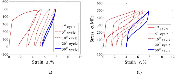
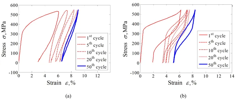
=0.2.The results obtained with various peak stresses, e.g., 450, 500 and 550 MPa are shown in Figs.
2-4. It is seen from the figures that the proposed model provides reasonable predictions to the
uniaxial transformation ratcheting of super-elastic NiTi SMA, compared with the experiments
observed by Kang et al. [31], as shown in Figs. 2(a)–4(a). The simulated results obtained from
simulated results with various peak stresses are shown in Figs. 2(b)–4(b). The figures show the
reasonability by the current FE model to predict the uniaxial transformation ratcheting of
super–elastic SMA, including the hysteresis loop curve, and the predicted peak and valley strain
The peak and residual strains of super–elastic SMA increase progressively during the initial
several loading cycles, and to a stable value since then. The nearly-total closed hysteresis loop
means that the strain increment happens in the tension loading is completely recoverable under the
following unloading. The closed hysteresis loop that still becomes smaller and smaller during the
further cyclic loading means that the dissipation energy decreases with the increase number of
loading cycles. Compared with the Kan-Kang's model with linear hardening law, as describe in
[29], the introduction of the cosine-type nonlinear function in the constitutive model enables the
predicted hysteresis loop with an apparent nonlinear feature that is more identical with the
experimental results .
Due to the introduced power function f
( )
AM
c
that is associated with the applied loadinglevel in the phase transformation ratcheting simulation, the model can reasonably predict the
variation of peak and valley strain with different applied loading level. It should be noted that the
introduction of the power equation with the coefficient of m and n, as described by Eqs (20a) and
(22a), can reasonably improves the prediction of peak strain and valley residual strain changing
experimental results yet, especially for larger loading levels. This indicates that the power
equation introduced in the proposed model dose still not fully reflect the highly nonlinear
relationship between the transformation ratcheting and the applied loading level. To achieve better
prediction results, it should be introduced a more complex function formulation with added more
material parameters.
(a) (b)
Fig. 1. Experiments and simulations for cyclic tension–tension with loading stress of 450 MPa: (a) experimental
result; (b) simulated result by proposed model.
(a) (b)
Fig. 2. Experiments and simulations for cyclic tension–tension with loading stress of 500 MPa: (a) experimental
(a) (b)
Fig. 3. Experiments and simulations for cyclic tension–tension with loading stress of 550 MPa: (a) experimental
result; (b) simulated result by proposed model.
To evaluate the current FE model, some experiments under the uniaxial cyclic loading
conditions is carried out and then are used to verify the validity of the proposed model in the
following discussions. The materials used in the new experiments are the super-elastic NiTi SMA
micro-tubes (Ni, 55.89% at mass, Xi’an Saite Metal Materials Development Co., Ltd., China). The
heat treatment process is different from the SMA used in Kang et al. [31], and then the start
temperature of martensite transformation Af is 282K lower than the test temperature 298K, the
original phase of the alloy is the pure austenite phase. Three different kinds of the uniaxial
nominal are controlled by axial load under cyclic tension–unloading with positive mean loads,
including cyclic tension–unloading tests with various applied peak stresses, e.g., 325, 365 and 405
at room temperature. The number of cycles is prescribed as 50, and the stress rate is prescribed as
20MPa/s. The material parameters used in the current FE model are determined by trial and error
method from the test data, as described in Section 2.2, and listed in Table 1 for the current FE
simulation.
Fig. 5(a)-7(a) show the experimental results of the uniaxial tension-unloading, which is used to
understand the basic performance of the NiTi SMA. It can be found from Fig. 6 that the start and
finish stresses of forward transformation shows decrease from 285 MPa to 225 MPa with the
increase number of loading cycles; while the start and finish stresses of reverse transformation are
from 345 MPa to320 MPa, respectively. After the unloading, a small residual strain is observed. It
is mainly caused by the martensite residual during phase transformation.
uniaxial transformation ratcheting of super-elastic NiTi SMA. The predicted peak and residual
strains, and their evolution characteristics are in fairly good agreement with the experimental
results obtained in the cyclic tension-unloading tests by current tests. Also, the dependence of
transformation ratcheting on the applied peak stress is reasonably predicted by the model due to
the employment of stress-dependent power function.
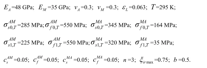
Table 2 Material parameters determined by tests of current work
A
E
=48 GPa;E
M=35 GPa;v
A=0.3;v
M =0.3;
L=0.063;T
=295 K;0,
AM s T
σ
=285 MPa;σ
AMf T0, =550 MPa;σ
s TMA0, =345 MPa;σ
MAf T0, =164 MPa;1,
AM s T
σ
=225 MPa;σ
AMf T1, =550 MPa;σ
s TMA1, =320 MPa;σ
MAf T1, =35 MPa;AM s
c
=0.05;c
AMf =0.05;c
sMA=0.05;c
MAf =0.05; n=3;
irmax=0.75;b
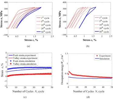
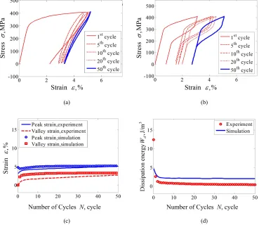
=0.5.From Figs. 5(c, d), 6(c, d) and 7(c, d), it is found that the peak and valley accumulation strains
increase with a exponential function law during the loading cycles, and the dissipation energy Wd
decreases on the contrary. The relative high degree of uniformity illustrates that the proposed
model could reasonably simulate the transformation ratcheting of SMA. After a certain cycles,
both of accumulation strains and dissipation energy show apparent change and quickly to a stable
value. These findings also agree with the conclusions simulated by Kan-Kang's model [33].
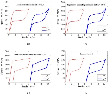
To further demonstrate the reasonability of the proposed constitutive model to predict the
transformation ratcheting of super-elastic NiTi alloy, two representative constitutive models
developed by [28-29] are discussed about their capability to predict the transformation ratcheting
in Fig. 8, respectively. The experimental data is obtained from [7]. The proposed model shows the
capability to predict the nonlinear feature of hysteresis loop by compared with the Kan-Kang's
model with linear hardening feature and the identical number of material parameters. Compared
with the Lagoudas's model, the proposed model can also predict the nonlinear feature of hysteresis
loop with the smaller number of material parameters. In addition, the proposed model can further
give a reasonable description for the cyclic deformation characteristic on a specific applied
loading level.
(a) (b)
(c) (d)
Fig. 5. Experiments and simulations for cyclic tension–unloading transformation ratchetting with constant loading
stress of 325 MPa: (a) experimental results; (b) simulated results; (c) curves of peak and valley strains vs. cycle
numbers; (d) curves of dissipation energy vs. cycle numbers.
(c) (d)
Fig. 6. Experiments and simulations for cyclic tension–unloading transformation ratchetting with constant loading
stress of 365 MPa: (a) experimental results; (b) simulated results; (c) curves of peak and valley strains vs. cycle
numbers; (d) curves of dissipation energy vs. cycle number.
(a) (b)
(c) (d)
Fig. 7. Experiments and simulations for cyclic tension–unloading transformation ratchetting with constant loading
stress of 405 MPa: (a) experimental results; (b) simulated results; (c) curves of peak and valley strains vs. cycle
(a) (b)
(c) (d)
Fig. 8. Stress–strain response of SMA to cyclic loading up to a constant value of stress: curves for the first and
50th cycles: (a) experimental results; (b) simulated results by Lagoudas's model; (c) simulated results by
Kan-Kang's model; (d) simulated results by proposed model.
It should be noted that the exponential function introduced in the proposed model correlated
the phase transformation ratcheting to the loading stress level still cannot fully reflect the high
nonlinear correlation between this ratcheting behavior and the loading stress level (e.g. Figs. 3 and
7). In order to achieve the better prediction results, it is necessary to consider the introduction of
more complex functional forms, and increase more material parameters. The evolution of the
phase transformation ratcheting strain is the focus of this paper. Therefore, this paper adopts a
simpler exponential function which can describe its general rule.
For some cases with unsatisfactory simulation results, the following are explained:
(1) In the phase transformation process, the mismatch of the internal strain of austenite and
martensite produces large local stress between the interface of austenite and martensite. The local
induced plasticity due to phase transformation is produced. However, because the grain size of the
selected material for experiment is relatively large, only the austenite near the interface between
austenite and martensite can be motivated the induced plasticity due to phase transformation at
some certain stress level. When the outer stress level reaches the starting critical stress of austenite
dislocation slip, that slip of the whole grain can be motivated. Therefore, by the comparison
between the experimental results of Figs. 2(a)-4 (a), it is known that the valley value strain of the
first circle show a significant nonlinear growth, and the same phenomenon can be observed from
the experimental results of Figs. 5-7.
(2) The phenomenological constitutive model proposed in this paper shows reasonability as
the amount of the induced plasticity is small. However, it does not consider the critical motivation
conditions of the starting stress of the dislocation slip of austenite. Therefore, when the stress level
of the external load reaches a certain value, for example, more than 500MPa, there exists a certain
difference between the proposed model and the experimental value in the prediction of the
hysteresis loop.
(3) Because of the above reasons, the prediction of ratcheting strain has a certain deviation in
the initial cycles when the external load is larger, and since then a better prediction result is
obtained. Although the proposed model has a certain numerical difference from the experimental
results in the prediction of individual conditions, the main characteristics of the described phase
transformation ratcheting behavior are in accordance with the experimental results. For this kind
of cyclic deformation with so strong nonlinearity, the accurate description of the hysteresis loop
should increase a lot of material parameters, which is not conducive to the application of the
engineering for the constitutive model.
5. Numerical examples for the analyses of preload force of SMA bolted joint
The preload force of SMA bolted joint is an important factor for the service properties of bolted joint, which also plays a crucial role in protecting the static and dynamic characteristics and
the locking and sealing properties of the whole SMA joint. However, in some conditions, it is
inevitable to reload the preload force of SMA bolt. This repeated process might decay the
excellent super-elastic of SMA bolt due to its phase transformation ratcheting of materials,
super-elastic SMA, a simplified FE model to analyze the repeated preloading process of SMA bolt
is derived, and used to calculate the repeated preloading process of SMA bolted joint, as a
numerical example. The member stiffness and the repeated preloading numbers are the influence
factors considered in this research.
A preset interference method is adopted in this research to simulate the bolt preloading, which
had successfully been used to simulate the preloading process of bolt in [32-34]. The preset
interference amount of
u
is built by shortening the distance of the bolt head and the nut inmodel as shown in Fig. 9. That means the preload force will be produced between the bearing
surfaces of the bolt head or nut and the member that will be integrated into one surface after bolt
preloaded.
(a) (b)
Fig. 9. Loading process and FE modeling of bolted joint: (a) before preloaded; (b) after preloaded.
5. 1 FE modeling for the preload process of SMA bolted joint
For simplicity, the FE model is only established by a half of the whole bolted joint structure in
this research due to its symmetrical characteristic on the whole structure size and load–bearing
feature of bolted joint along the contact surface of the contacted members. The nodes (e. g. node
numbers of 2 and 4) close to the side of bearing surface of one member are fixed as the restrained
end. For the specific preloading process, the initial parameters for simulation should be input into
model firstly, such as the elastic modulus of material, cross sectional area and effective length of
bolt bar, to calculate the tensile stiffness of bolt, and the compression stiffness of members. The
initial value of
u
. The target of the iterative calculation is to reach the force equilibriumconditions, i.e.
F
b
F
m
F
p0 from initial force conditionsF
b
F
m
0
. For each sub-step ofiterative calculation, a sub tension force is applied on the bolt, and the sub compression force is
used on the member. The amount of deformation for each iterative sub–step are set as
u
b andm
u
for bolt and member, respectively. For the absolute coordinates value of nodes 2 and 4 foreach iterative sub–step calculation, the following deformation equation gets to work:
1
1
b b b
n n n
m m m
n n n
b m
n n n
u
u
u
u
u
u
u
u
u
(42)
in which, n is number of iterative sub–step.
The amount of interference
u
decreases gradually with iterative calculation in progress.For the case of
u
0
, the amount of penetration between the bearing surfaces of the bolt or nutand the member is zero, and the iteration is terminated. It should be noted that the target
preloading force
F
p0 should be continuously adjusted the amount of initial interference
u
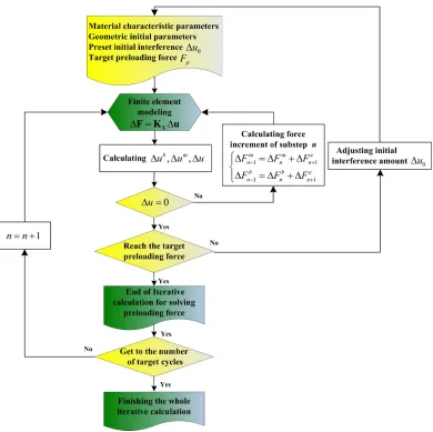
0bytrial and error method. The specific implementation process is shown in the flow chart of Fig. 10.
It should be noted that the SMA bolt element and the member element are independent for
each other in FE modeling. It means that the force increments of iteration for
F
nm and
F
neare applied on the SMA bolt element and the member element, respectively, in spite of
m e
n n
F
F
. Then the deformations for each element are calculated independently until theFig. 10. Flow chart of analysis of the repeated cyclic preloading
The equilibrium equation of SMA bolt or member can be expressed using the standard FE
assembly operation:
F K
U
u
(43)Where,
F
indicates the increment of nodal force vectors of bar elements of the FE model,
u
is the nodal displacement vectors,K
U is the stiffness matrices.The FE model of a member is shown in Fig. 9. It can be seen that the member elements consist
of the nodes 1 and 2. The node 2 is the restrained end, and the node 1 is the force applied end of
member element. Thus, Eq. (43) can be further decomposed into
11 12
1 1
21 22
2 2
u u
u u
F
K
K
u
where,
u
1,u
2 andF
1,F
2 are the displacements and the forces of the node 1 and 2,respectively.
F
1 andF
2 are a pair of equilibrium forces with equal magnitude in oppositedirections.
K
11u ,K
12u ,K
13u ,K
21u andK
22u are the partitioned matrices of matrixK
mU.Since the member is equivalent to a bar element in the FE model, the relationship between
force vector and displacement vector of the node i can be written as
0
0
0
=
m mm m m m m m
m m m
E A
L
L
k L
L
L
L
L
x
x
F
(45)
where,
A
m is the equivalent cross section area of the member element.L
m0 are the initialunstressed length of member element,
E
m is the elastic modulus of member element,k
m is thecompression stiffness of member element.
F
m is the force vector of member element,i j
x x
x
depicts the relative nodal position denoted byx
i andx
j in the global frame. i,j=1 or 2 are the node numbers of member element.
L
m
i
j
T i
j
1/2
x
x
x
x
is thestressed length of the member element after deformed.
With the first order Taylor expansion of Eq. (45), it can be derived as
m m
F
F
x
x
(46)Since
F
jF
i, the incremental relationship between nodal force and element length can beexpressed as
m m m
F
K u
where, m i
j
F
F
F
, i i m j j
u
x
u
u
x
, andk
k
k
k
m m m m m
K
The stiffness matrix of one node can be obtained by the differential calculation as
T T
0 0 0
3 3
2 2
0
k
m m m m m m m m m m mm m
m m m m m m m
E A
E A L
L
k L
L
L
k
L
L
L
L
L
L
L
F
xx
xx
I
I
x
(47)where,
I
3 is 3×3 is identity matrix.The equilibrium equation of member structure can be achieved using the standard FE assembly
m
m m
F K
u
K
U
u
(48)The boundary condition of member element during the preloading of bolt is
u
4=0
. Thus,33 3 3 4 3 u
K
u
F
F
F
(49)The further derivation gives
1 33
3 u 3
u
K
F
(50)According to the above calculation, the deformation of each element of member and the
relationship of stress and strain are obtained.
As for the SMA bolt, the FE model of bolt is established simplistically to be a bar element. As
shown in Fig. 9, the SMA bolt element consists of nodes 3 and 4. Therefore, Eq. (43) can be
divided into 33 34 3 3 43 44 4 4 u u u u
F
K
K
u
F
K
K
u
(51)where,
u
3,u
4 andF
3,F
4 are the displacements and the forces of the nodes 3 and 4,respectively.
F
3 andF
4 are a pair of equilibrium forces with equal magnitude in oppositedirections.
K
33u 、K
34u 、K
u43 andK
44u are the partitioned matrices of matrixK
bU.The boundary condition of SMA bolt element during the preloading of bolt is
u
4=0
. Thus,33 3 3 4 3 u
K
u
F
F
F
(52)The further derivation gives
1 33
3 u 3
u
K
F
(53)Since the FE model of SMA bolt is established as just one bar element, it is no need to carry out
the assembly calculation of FE modeling. Therefore,
b
b b
F K u
K
U
u
(54)where,
k
k
and
k
sma b
K
U .sma U
K
is the stiffness matrix of node in SMA bolt element, and can be seen inEq. (48). It is given by comparing Eq. (51) and Eq. (54),
3
4
b
F
F
F
, 34
b
u
u
u
,33 34
43 44
u u
b
u u
U
K
K
K
K
K
(55)5.2 Simulations and Results
In this section, it is given a numerical example about the repeated preload process of SMA
bolted joint based on the above FE model. The M6 NiTi SMA bolt is selected in this research.
Upper and lower members are completely identical, including dimensional size and materials. The
calculation approach of the member stiffness can be cited from the references in Motosh and
Nassar[35-36] who had developed the analytical model to describe the accurate member stiffness
relatively. The stiffness value is calculated as km=4×10⁸ N·m–1 as a reference with the dimensional
sizes of height 50mm and diameter 30mm, and the elastic modulus 70×109 Pa and Poisson ratio
0.28 of selected aluminum.
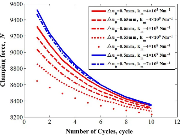
FE simulations are conducted for ten transverse loading cycles. Figure 11 shows the
stress–strain hysteresis loops obtained from the bolt bar for different amount of preset interference,
i.e. △u0=0.5mm, △u0=0.55mm, △u0=0.6mm, △u0=0.65mm and △u0=0.7mm, that correspond
to the initial preload forces of SMA bolt as Fp0=8.65kN, Fp0=8.86kN, Fp0=9.04kN, Fp0=9.19kN
and Fp0=9.32kN. It can be found that the SMA material of the bolt experienced the cyclic
ratcheting with increasing number of repeated preloading cycles. The repeated cyclic preloading
will produce lower clamping force of bolt with the same amount of preset interference until
tension stress value of bolt is close to the martensite start stress. Similar to the materials ratcheting
behavior, the clamping force of SMA bolt experiences the great attenuation during the initial
several loading cycles and tends to be stable with a very small value since then. It should be noted
that although the attenuation rate of the clamping force of bolt increases with the increase of initial
preload force of bolt, the larger initial preload force of bolt shows higher residual clamping force
after experienced cycle preloading. After experienced nearly five loading cycles, the martensite
phase produced in initial preload will be close to disappearance. It can also be found from Fig. 12
that the higher member stiffness would improve the reduction of preload force under repeated
stiffness in this research is higher than km=7×10⁸ N·m–1, the initial preload and its attenuation rate
are not changed obviously. It means that the effectiveness of the optimum design from the
standpoint of adjustment of km will not be too obvious.
(a) △u0=0.5mm, km=4×10⁸ N·m–1 (b) △u0=0.55mm, km=4×10⁸ N·m–1
(c) △u0=0.6mm, km=4×10⁸ N·m–1 (d) △u0=0.65mm, km=4×10⁸ N·m–1
(g) △u0=0.7mm, km=1×10⁹ N·m–1
Fig. 11. Curves of stress–strain responses on bolt bar under different load cases
Fig. 12. Clamping force reduction of bolt with increasing loading cycles under different load cases
5. Conclusions
In this work, a phenomenological constitutive modeling and its FE implementation of
super–elastic SMAs is carried out to simulate the transformation ratcheting behaviors of the
super–elastic SMA undergoing cyclic loading, the conclusions are obtained as follows:
(1) The assumed cosine–type phase transformation function considering the initial martensite
evolution is verified to be candidate for predicting the contributions of cyclic accumulation of
residual martensite caused by incomplete reverse transformation, and the nonlinear behavior of
transformation stresses can be controlled by accumulated martensite volume fraction as a internal
variable. The correlation between the applied loading level and the transformation ratcheting is
also able to be captured by the proposed model.
(2) A FE model derived by return-mapping method is then to analyze the attenuation law of the
clamping force of SMA bolt experiences as numerical example. It is found that the great
attenuation of clamping force of SMA bolt happens during the initial several loading cycles and
tends t
![Fig. 1. Typical tension–unloading stress–strain curve of materials [29]](https://thumb-us.123doks.com/thumbv2/123dok_us/1004373.1600276/14.612.207.420.138.291/fig-typical-tension-unloading-stress-strain-curve-materials.webp)
![Table 1 Material parameters observed by Kang et al. [31].](https://thumb-us.123doks.com/thumbv2/123dok_us/1004373.1600276/15.612.112.447.90.205/table-material-parameters-observed-kang-et-al.webp)