MULTI-LAYER GRID REFINEMENT
METHOD
TSUN-ZEE MAI1 1
Department of Mathematics, University of Alabama
Tuscaloosa, AL. 35487, USA
Email: [email protected]
LEINA WU2 2
Department of Mathematics and Computer Information Systems, Queens University of Charlotte
Charlotte, NC. 28274, USA Email: [email protected]
Abstract:
The uniform grid scheme has been widely used to solve a partial differential equation. Due to the extreme large linear systems generated by the uniform grid scheme, a lot of computation time is required. To improve the efficiency of the uniform grid scheme, a more economical method is desirable. In this paper, we propose a multi-layer grid refinement method for solving a partial different equation over a rectangular domain with Dirichlet boundary conditions. Numerical experiments demonstrate that the efficiency has been improved significantly, and the accuracy is satisfactory.
Keywords: multi-layer grid refinement method; domain decomposition; partial differential equation; iterative methods
1. Introduction
Groundwater problems [5, 6, 10] have always been around our daily lives. Contamination of the groundwater source can cause serious environmental hazards. Regions with sinkholes can be particularly susceptible to the groundwater contamination. Once water enters a sinkhole, it receives litter filtration or chance for degradation of the chemicals. Then the water will migrate down to the groundwater table where it will disperse in the groundwater and migrate in the direction of the groundwater flow.
Researchers from geological sciences have been conducting studies about the hydraulic heads and contamination spreading problems. For instance, if there is a rectangular domain where the boundary conditions are given, and the initial contamination value at the sinkhole is also known, it is desired to find out the contamination values in the region around the sinkhole. Researchers have been using the model
“MODFLOW” to solve hydraulic head problems by a two-step procedure [5]. First, the whole region is
discretized into one uniform coarse grid domain, and the solution to each grid within the region is solved. Once the solution to the whole region is obtained, a second region which is of most interest around the sinkhole is constructed. This region is covered with fine grids and the “interface” boundary values of this region are interpolated from the solution attained previously by the first step. Another linear system corresponding to the second region is then produced and solved.
method based on the incomplete Cholesky factorization [1, 4] namely incomplete LU (ILU) is used and accelerated by the BICGSTAB procedure [7]. Since the computational time is proportional to the size of the generated linear system, our goal is to reduce the size of the linear system without sacrificing too much accuracy Therefore, we place fine grids over the interested domain and coarse grids outside the interested domain in the region. Modifications are needed for approximating the partial derivatives of the points that lie on the boundaries of the interface of the interested and less interested domains. In this paper two spatial dimensions are considered. We believe that three spatial dimensions can also be applied, see [3].
2. Problem Descriptions and Grid Refinement Method
In this section, we describe a grid refinement method for solving a partial differential equation (PDE) defined on a rectangular region of the form
( , ) xx ( , ) yy ( , ) x ( , ) y ( , ) ( , )
A x y u C x y u D x y u E x y u F x y uG x y (1)
where A, C, D, E, F are functions of x and y, with Dirichlet boundary conditions on the boundaries. A numerical solution of the partial differential equation is based on a finite difference scheme. In order to have an accurate approximation, the grid size must be very small. In this case, the generated linear system becomes very large and sparse. The computation time is substantial. More often we are only interested in some small domains in the region. It is not necessary to put very small grids on the less interested domains. It motivates us to investigate the multi-layer grid refinement method so that we may balance the accuracy and the computation time.
2.1. Multi-Layer Grid Refinement Method
The idea of the multi-layer grid refinement method is to decompose the original spatial domain into several subdomains. For simplicity, we describe the two-layer method using two subdomains, namely the interested domain and the less-interested domain. The coarse grids are put on the less-interested domain; therefore, it is also referred to as the coarse grid domain. The fine grids are put on the interested domain which is then also referred to as the fine grid domain. Once the grids are placed, one linear system is generated. Then we are able to solve both subdomains simultaneously. We note that the fine grid domain can be formed in a rectangular shape or in other shapes, such as L shape or circular shape. In this research, we focus on the rectangular shape. We also note that the fine grid domain can be placed in anywhere within the original region to fit physical needs. Again for simplicity, we assume that the fine grid domain is located in the center of the region, see Fig.1.
Fig.1 Grid pattern for the two-layer scheme
In order to obtain the difference equation, the finite difference scheme with the 5-point stencil is used; see Fig.2 and Fig.3.The mesh sizes ∆x1,∆x2,∆y1,∆y2 may be different. However, we assume that within
directions are the same, i.e. ∆x1 = ∆x2 = ∆y1 = ∆y2. We refer to these points as regular points. We let H denote
the coarse mesh size and let h denote the fine mesh size. Therefore, for the regular points, the stencil is illustrated by Fig.3.
Fig.2. 5-point stencil for the finite difference method Fig.3. 5-point stencil for the finite difference method with same mesh sizes
It is well known that central finite difference schemes for the partial derivatives uxx, uyy , ux, uy are
given by (2),
2 2
2 2
, ,
, .
2 2
E W C N S C
xx yy
E W N S
x y
u u u u u u
u u
k k
u u u u
u u
k k
(2)
All of those formulas are of order . For the regular points of each subdomain, the partial differential
equation can be discretized using the above formulas. However, in order to form one linear system by using two different grid sizes, it is necessary to consider the “inner boundaries” or the interfaces between the coarse grid domain and the fine grid domain. The central difference formulas (2) are no longer feasible for the discretization on the interface boundary points.
There are two types of interface boundary points. Some boundary points are next to coarse grid points. Some are not. We refer to these points as irregular points. The boundary points with adjacent coarse grids are illustrated in Fig. 4 .
Fig.4 . 5-point stencil for boundary points with adjacent coarse grids
In this situation un, uc and us are boundary points, uw is the adjacent coarse point, and ue is the
adjacent fine grid point. By using the Taylor series expansion, we may obtain the finite difference approximations for uxx, uyy , ux, uy as
x2
y2
x1
y1
Uc Uw
Us
Ue Un
K K
K K
Uc Uw
Us
Ue Un
h
h h H uw
us
ue
un
2
2 2 2 2
2 ( ) 2
, ,
( )
( )
, .
( ) 2
W E C N S C
xx yy
E W C N S
x y
h u H u h H u u u u
u u
h H h H h
H u h u H h u u u
u u
h H h H h
(3)
Putting these approximations into (1), we obtain the difference equation
0u x y( , ) 1u x h y( , ) 2u x y h( , ) 3u x h y( , ) 4u x y h( , ) G
(4)
where
1 2 2 3 4 2
0 2
2 2
, , , ,
( ) 2 ( ) 2
2 ( ) 2
.
A HD C E A hD C E
h h H h h H h H h h
A H h D C
F
hH h
(5)
We assume that . Then and can be written as
1 22 , 3 22
(1 ) (1 )
A hD A hD
h h
(6)
and α0 becomes
0 2 2
2 ( 1) 2
.
A h D C
F
h h
(7)
The other kind of boundary point that is not adjacent to a coarse grid point is shown in Fig.5.
Fig.5. 5-point stencil for boundary points without adjacent coarse grids
The discretization formula proposed by Jun and Mai [2] in the MIP algorithm has been applied and
modified as given below. For the case illustrated in Fig.5, there is no grid to the left of uc. The finite
2
2 2 2 2
2 ( ) 2
,
( )
( )
,
( ) 2
b E C N S C
xx yy
E b C N S
x y
h u l u h l u u u u
u u
h l h l h
l u h u l h u u u
u u
h l h l h
(8)
where ub is the value on the boundary of the region defined by the Dirichlet conditions of the partial
differential equation, l is the distance between uc and ub. The same principle is extended to other three
boundaries.
2.2. The Accuracy Analysis of Grid Refinement Method
The general difference equations on the left interface between the fine grid domain and the coarse grid domain (except the corner points) can be written as
0uC1uE2uN3uW4uS 0 (9)
where
1 2 2 2 3 2 4 2
0 1 2 3 4 2
2 1 2 1
, , , ,
(1 ) (1 )
2(1 )
.
h h h h
h
(10)
We note that here we assumelh. After solving uCfrom the equation (9), we obtain
1 1 1 1
.
1 1 1 1 2 2
C E W N S
u u u u u
(11)
It is easy to see that the expression in the first bracket represents a linear interpolation of uEand uW.
Meanwhile, we may consider the expression in the second bracket to be a linear interpolation of uN and uS.
The accuracy of the linear interpolation can be found in the following lemma [9].
LEMMA 2.1. Let , and be the linear interpolation of with and
. Then if | | for all , and some constant M, then
| | (12)
Since uc is the approximation of the exact value u, the error can be computed by
1 1 1 1
1 1 1 1 2 2
1 1 1 1
.
1 1 1 1 2 2
C E W N S
E W N S
u u u u u u u
u u u u u u
(13) By LEMMA 2.1, we have
2 2
1 (1 )
1 E 1 W 8
h
u u u M
and
2
1 1
2 N 2 S 2
h
u u u M
where
2 2
2 2
max u , u
M
x y
over the interval [a, b]. Therefore, the total error of the approximation
u
Ccan be combined as
2 2 2
2
1 (1 )
1 8 1 2
.
8 2(1 ) 8
C
h M h
u u M
Ml Ml h M
h
(15)
This indicates that the accuracy of the approximation on the left interface becomes the first order of h. Similarly, the same order of accuracy can be obtained on all the other interfaces and corner points. The accuracy on the interface points is then combined with the regular points that are of the second order accuracy. Thus we obtain the accuracy for the whole grid refinement scheme is of the first order. We summarize the result in a theorem.
THEOREM 2.1. The accuracy of the grid refinement scheme with the treatment on the interface points by (3)
and (8), along with the difference scheme (2) for the regular points for solving Eq. (1), is of first order.
3. Numerical Experiments
We perform numerical experiments using the grid refinement method on model problems. We focus on the convergence, accuracy, and efficiency of the grid refinement method.
3.1. Model Problems
We first introduce the model problems for our numerical experiments.
3.1.1. Model Problem 1 (MP1).
uxxuyy 0
(16)
over the region Ω= [0, 1] × [0, 1]. The boundary conditions are given by
u(0, )y cosy,
1 (1, ) cos ,
u y e y u x( ,0)ex,u x( ,1)excos1.
(17)
The exact solution is uexcosy.
3.1.2. Model Problem 2 (MP2).
uxxuyy D x y u( , ) xE x y u( , ) y u G x y( , ) (18)
whereD x y( , )sin sinx y, E x y( , )cos cosx yand G x y( , ) sin cos ,x y
over the region Ω = [0, 1] × [0, 1]. The boundary conditions are given by
u(0, )y 0, (1, )u y sin1cos ,y u x( , 0)sinx, ( ,1)u x sin cos1.x (19)
The exact solution isusin cosx y.
In this paper, we use the stopping criteria ( )
2
2 i
u u
u
where u(i) is the approximate solutions at
3.2. Efficiency of the Two-layer Scheme
In the previous section, we have proven that the grid refinement method using the treatment of inner boundary points similar to the MIP procedure is of order h. Table 1 shows the exact errors that indicate the first order accuracy. When H and h are halved, the error is reduced by approximately 1/2.
Table 1. Error with various H and h for MP1 and MP2
H h Matrix
Size
Error on the interested
domain (MP1)
Error on the interested
domain(MP2)
1/10 1/20 97 4.4838E-04 5.6406E-04
1/20 1/40 417 2.3312E-04 2.9620E-04
1/40 1/80 1729 1.2434E-04 1.5867E-04
1/80 1/160 7041 6.5710E-05 8.3674E-05
Even though the method is of first order, it is very efficient. For example, if the solution of a dense set of points in the interested domain is needed, then a very fine mesh must be placed on the entire region. This leads to a huge linear system. The computation time is significant. On the other hand, the grid refinement method only places the same fine mesh size on the smaller interested domain; the rest of the region can be covered with larger mesh size grids. In such a case, a smaller linear system is generated and less computation time is subsequently needed.
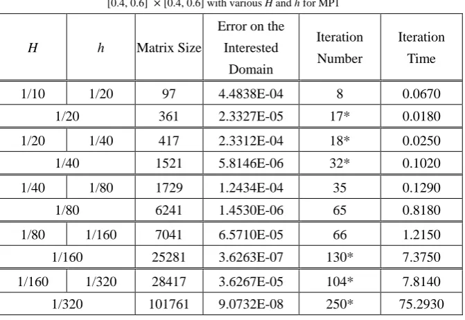
Table 2. Computation time and the 2-norm error on the interested domain [0.4, 0.6] × [0.4, 0.6] with various H and h for MP1
H h Matrix Size
Error on the
Interested Domain
Iteration Number
Iteration Time
1/10 1/20 97 4.4838E-04 8 0.0670
1/20 361 2.3327E-05 17* 0.0180
1/20 1/40 417 2.3312E-04 18* 0.0250
1/40 1521 5.8146E-06 32* 0.1020
1/40 1/80 1729 1.2434E-04 35 0.1290
1/80 6241 1.4530E-06 65 0.8180
1/80 1/160 7041 6.5710E-05 66 1.2150
1/160 25281 3.6263E-07 130* 7.3750
1/160 1/320 28417 3.6267E-05 104* 7.8140
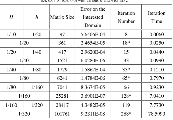
Table 3. Computation time and the 2-norm error on the interested domain [0.4, 0.6] × [0.4, 0.6] with various H and h for MP2
H h Matrix Size
Error on the
Interested Domain
Iteration Number
Iteration Time
1/10 1/20 97 5.6406E-04 8 0.0060
1/20 361 2.4654E-05 18* 0.0250
1/20 1/40 417 2.9620E-04 15 0.0440
1/40 1521 6.0280E-06 33 0.0990
1/40 1/80 1729 1.5867E-04 35* 0.1210
1/80 6241 1.4784E-06 65* 0.7970
1/80 1/160 7041 8.3674E-05 66 0.9230
1/160 25281 3.6901E-07 128* 7.0410
1/160 1/320 28417 4.3482E-05 119 7.7730
1/320 101761 9.2311E-08 268* 78.5990
Table 2 and Table 3 show the accuracy and efficiency of the grid refinement scheme for MP1 and MP2, respectively. There are five groups of data in Table 2 and Table 3. The first row of each group indicates the grid refinement scheme, and the second row indicates the uniform grid scheme over the entire region. We assume that [0.4, 0.6] × [0.4, 0.6] is the interested region. The interested region is covered by the same fine grids with size h for both schemes. The non-interested region is covered by coarse grids with mesh size H that is twice of h for the two-layer scheme. The results show that the accuracy of the fine grid scheme within the interested area is slightly less than that of the uniform grid scheme; but the iteration time spent on finding solutions, is dramatically reduced. From the tables, it can be seen that both the size of the linear system and the number of iterations are reduced significantly. Because of the smaller linear system and less number of iterations, the computation time is significantly reduced. We note that the iteration numbers with (*) in the subsequent tables indicate the half-iterations produced by the “bicgstab” from MATLAB.
3.3. Geology Simulation
We now attempt to apply the grid refinement method on a geology problem concerned with the groundwater transport model. For the transport model, the governing equation involves ux and uy that serve
the velocity terms. We consider the PDE
· x 0 (20)
over the region Ω = [0.5, 20.5] × [0.5, 20.5] with the zero boundary conditions. It is assumed that q is the point sink/source at the center of the region. In this research, we assume that the coefficients D and E are constants that contribute the velocity of the flow. It is known that in order to have a numerical stability, the
Peclet number Pemust be less than or equal to 2, see [10]. For the uniform grid scheme,
· ∆ 1 (21)
should be satisfied, where represents the uniform grid size. When the grid refinement scheme is used,
we let D be the maximum of D(x, y) and E(x, y) and we let ∆ represent the minimum of H and h. So (21) becomes
max{ ( , ), ( , )} min{ , } 1.D x y E x y H h (22)
Let us use a hypothetical model with the equation
10 5 0
over [0.5, 20.5] × [0.5, 20.5] andThe function q is defined below as the sink/source in our experiments.
10, at , 10.5,10.5
0, elsewhere. (24)
Table 4 shows the computation time for obtaining the solution using the uniform grid scheme and the two-layer scheme. The interested region in this experiment is set to be [8.5, 12.5] × [8.5, 12.5].
Table 4. Computation time for Geology Simulation
H h Size Iteration Time
1 1/10 2017 1.141
1/5 1/10 11041 0.956
1/10 1/10 39601 4.958
1 1/16 4561 6.911
1/2 1/16 5665 9.42
1/16 1/16 101761 28.722
1/5 1/20 15921 14.699
1/10 1/20 44481 19.062
1/20 1/20 159201 65.222
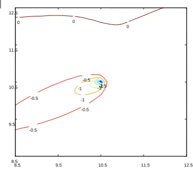
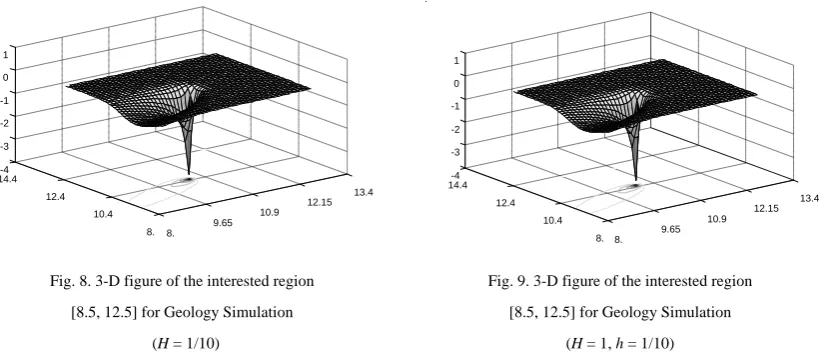
With h = 1/10, the contour plots of the solution over the interested region are given in Figures 6 and 7, where Figure 6 is the plot from the uniform grid scheme. Moreover, the 3-D plots are given in Figure 8 and Figure 9 for the uniform grid scheme and the two-layer scheme, respectively. From the figures, we can see that they are very alike, but the computation times are very different. In general, the computation time required by the uniform grid scheme is ranging 4 to 15 times more than the two-layer scheme.
Fig. 6. Contour figure of the interested region [8.5, 12.5] for Geology Simulation
(H = 1/10)
Fig. 7. Contour figure of the interested region [8.5, 12.5] for Geology Simulation
(H = 1, h = 1/10)
-3-2-1.5
-1 -1
-0.5
-0.5
-0.5
-0.5
0 0
0
8.5 9.5 10.5 11.5 12.5
8.5 9.5 10.5 11.5 12.5
-2-1.5
-1 -1
-0.5
-0.5
-0.5
-0.5
0
8.5 9.5 10.5 11.5 12.5
8.5 9.5 10.5 11.5 12.5
Fig. 8. 3-D figure of the interested region
[8.5, 12.5] for Geology Simulation (H = 1/10)
Fig. 9. 3-D figure of the interested region
[8.5, 12.5] for Geology Simulation (H = 1, h = 1/10)
4. Conclusions
In this research, we study the commonly used uniform grid scheme and propose the grid refinement scheme for solving a partial different equation over a rectangular domain with Dirichlet boundary conditions. The grid refinement technique can be applied to some irregular domains, such as circular and L-shape domains. We also study some variant of the grid refinement schemes, such as the two-layer scheme and the three-layer scheme. Numerical experiments demonstrate that the efficiency has been improved a great deal when the uniform grid scheme and the grid refinement scheme are compared. Even though the accuracy of the proposed method has been shown of the first order, the accuracy is satisfactory. Especially when we focus on the interested region, the accuracy is very comparable to the fine uniform grids accuracy, but the computation time is reduced dramatically. A geological simulation is also conducted. With a huge efficiency improvement, the solution obtained by the grid refinement scheme is very comparable to the solution obtained by the uniform grid scheme.
References
[1] Horn R. A.;C. R. Johnson. (1985). Matrix Analysis, Cambridge University Press, Cambridge, England. [2] Jun Y.; Mai Tsun-Zee (2006): ADI method-Domain decomposition, Appl. Numer. Math., 56, pp.1092 – 1107.
[3] Jun Y.; Mai Tsun-Zee (2009): Numerical analysis of the rectangular domain decomposition method, Communication in Numerical Methods in Engineering, 25, pp.810 – 826.
[4] Meijerink J. A.; Van Der Vorst H. A..(1977): An iterative solution method for linear systems of which the coefficient matrix is symmetric M-matrix, Math. Comput. 31, pp. 148 – 162.
[5] Mehl S.; Hill M.C.(2004): Three-dimensional local grid refinement for block-centered finite-difference groundwater models using iteratively coupled shared nodes: a new method of interpolation and analysis of errors, Advances in Water Resources, 27, pp. 899 – 912.
[6] Press W. H.; Flannery B. P.; Teukolsky S. A; Vetterling W. T. (1992): LU Decomposition and Its Applications. Numerical Recipes in FORTRAN: The Art of Scientific Computing. Cambridge University Press, Cambridge, England.
[7] Van Der Vorst H. A.(1992: Bi-CGSTAB: A fast and smoothly converging variant of Bi-CG for the solution of nonsymmetric linear systems, SIAM J. Sci. Statist. Comput. 13, pp. 631 – 644.
[8] Young D. M. (1971). Iterative Solution of Large Linear Systems, Academic Press.
[9] Young D. M.; Gregory R. T. (1972). A Survey of Numerical Mathematics, Addison-Wesley Educational Publishers Inc. [10] Zheng C.; Bennet G.D.(2002). Applied Contaminant Transport Modeling, John Wiley and Sons, New York.
8. 9.65
10.9
12.15 13.4
8. 10.4 12.4 14.4-4
-3 -2 -1 0 1
8.
9.65 10.9 12.15
13.4
8. 10.4 12.4 14.4-4