University of Pennsylvania
ScholarlyCommons
Publicly Accessible Penn Dissertations
1-1-2013
A Three Layered Framework for Annual Indoor
Airflow CFD Simulation
Yue Wang
University of Pennsylvania, [email protected]
Follow this and additional works at:http://repository.upenn.edu/edissertations
Part of theComputer Sciences Commons,Environmental Engineering Commons, and the
Mechanical Engineering Commons
Recommended Citation
Wang, Yue, "A Three Layered Framework for Annual Indoor Airflow CFD Simulation" (2013).Publicly Accessible Penn Dissertations. 813.
A Three Layered Framework for Annual Indoor Airflow CFD Simulation
Abstract
Computational fluid dynamics (CFD) is one of the branches of fluid mechanics that uses numerical methods and algorithms to solve and analyze problems that involve fluid flows. Computers are used to perform the millions of calculations required to simulate the interaction of liquids and gases with surfaces defined by boundary conditions. Indoor airflow simulations are necessary for building emergency management, preliminary design of sustainable buildings, and real-time indoor environment control.
The simulation should also be informative since the airflow motion, temperature distribution, and contaminant concentration is important. However, CFD computation is usually time-consuming, and not suitable for simulating real-time indoor air movement. Many researchers are concentrating on both hardware utilization and CFD algorithms, to make simulation much faster. Fast flow simulations are important for some applications in the building industry, such as the conceptual design of indoor environment, or they are coupled with energy simulation to provide deep analysis on the performance of the buildings. Such application does not require the same high level of accuracy as traditional CFD simulation because it only requires conceptual or semi-accurate distributions of the flow but within a short computing time. However, year round simulation is needed rather than the analysis of two or three extreme cases in order to help the designer investigate the problem clearly. To meet these special needs, an efficient and informative fluid simulation method is needed to provide fast airflow simulation with an inevitable but nominal compromise in accuracy.
This research provides a comprehensive workflow for the designer to simulate and analyze the annual indoor environment. In addition to the hardware acceleration deployed, fast fluid simulation algorithm is developed, and a machine learning based interpolation is used to allow the simulation coverage to be conducted annually. The outcome of this research is a methodology that allows the annual simulation time similar to the one used to perform two or three extreme cases of simulation using current methods.
Degree Type Dissertation
Degree Name
Doctor of Philosophy (PhD)
Graduate Group Architecture
First Advisor Ali M. Malkawi
Subject Categories
A THREE LAYERED FRAMEWORK FOR
ANNUAL INDOOR AIRFLOW CFD SIMULATION
Yue Wang
A DISSERTATION
in
Architecture
Presented to the Faculties of the University of Pennsylvania
in
Partial Fulfillment of the Requirements for the
Degree of Doctor of Philosophy
2013
Supervisor of Dissertation
Ali M. Malkawi
Professor of Architecture
Graduate Group Chairperson
David Leatherbarrow
Professor of Architecture; Chair, Graduate Group in Architecture
Dissertation Committee
To Prof. Malkawi
Acknowledgment
I could never find adequate words to express my gratitude to my advisor
Professor Ali Malkawi. With his vision into the research frontier, unreserved
support, constructive advice, broad knowledge, diligence, and great sense
of humor, he has been my role model since my first day of graduate study.
I appreciate his profound belief in my work and abilities. I would like to
extend my sincere thanks to my committee members for their invaluable
advice and suggestions: Prof. Paulo E. Arratia and Dr. Yun Kyu Yi.
This research has received help from scholars in Purdue University.
Some part of the FFD simulations in this research was performed using a
ABSTRACT
A THREE LAYERED FRAMEWORK FOR
ANNUAL INDOOR AIRFLOW CFD SIMULATION
Yue Wang
Ali Malkawi
Computational fluid dynamics (CFD) is one of the branches of fluid
mechanics that uses numerical methods and algorithms to solve and
an-alyze problems that involve fluid flows. Computers are used to perform
the millions of calculations required to simulate the interaction of liquids
and gases with surfaces defined by boundary conditions. Indoor airflow
simulations are necessary for building emergency management, preliminary
design of sustainable buildings, and real-time indoor environment control.
The simulation should also be informative since the airflow motion,
tem-perature distribution, and contaminant concentration is important.
How-ever, CFD computation is usually time-consuming, and not suitable for
simulating real-time indoor air movement. Many researchers are
concentrat-ing on both hardware utilization and CFD algorithms, to make simulation
much faster. Fast flow simulations are important for some applications in
the building industry, such as the conceptual design of indoor environment,
the performance of the buildings. Such application does not require the
same high level of accuracy as traditional CFD simulation because it only
requires conceptual or semi-accurate distributions of the flow but within
a short computing time. However, year round simulation is needed rather
than the analysis of two or three extreme cases in order to help the designer
investigate the problem clearly. To meet these special needs, an efficient
and informative fluid simulation method is needed to provide fast airflow
simulation with an inevitable but nominal compromise in accuracy.
This research provides a comprehensive workflow for the designer to
simulate and analyze the annual indoor environment. In addition to the
hardware acceleration deployed, fast fluid simulation algorithm is developed,
and a machine learning based interpolation is used to allow the simulation
coverage to be conducted annually. The outcome of this research is a
methodology that allows the annual simulation time similar to the one used
Table of Contents
1 Introduction 1
1.1 Motivation 1
1.2 Problem statement 2
1.3 Background 3
1.4 Dissertation outline 5
2 GPU Accelerations 7
2.1 Introduction 7
2.2 Methodology 14
2.3 Speeding up simulation using OpenCL 17
2.4 Case studies 24
2.4.1 Cavity case benchmark 24
2.4.2 Pure conjugate gradient benchmark 25
2.4.3 Hot room case 28
2.5 Conclusions 29
3 FFD Accelerations 31
3.1 Introduction 31
3.2 Case study 35
3.3 Conclusions 36
4 Strategy Planning Algorithm 39
4.1 Introduction 39
4.2 Predicting the convergence speed 42
4.3 Minimal simulation by case reuse 49
4.3.1 Predicting output differences 51
4.3.2 Assigning edge values in a graph 52
4.3.3 Strategy planning module 53
4.3.4 Multivariate interpolation 55
4.4.1 Introduction 56
4.4.2 Regression and prediction 57
4.4.3 The strategy graph 61
4.4.4 Solving cases that can be directly interpolated 62
4.4.5 Simulate certain cases after interpolation 64
4.4.6 Perform simulation on the remaining cases 66
4.5 Discussion 70
4.6 Conclusions 74
5 Conclusions 76
5.1 Summary 76
5.2 Precision and speed tradeoff 78
5.3 Limitation of this research 79
A Vector Difference Definition 81
Bibliography 85
List of Tables
4.1 Four selected cases in annual simulation 46
4.2 Summary of relationship between input difference and
iterations needed to converge from one case to another 48
4.3 Input parameters for caseid200, 8744 and 344 63
4.4 Input parameters for caseid8430, 20 and 188 66
4.5 Input parameters for caseid20 and 1664 68
5.1 Three Layered framework. The estimated total speed-up
List of Figures
2.1 OpenFOAM simulation workflow (All the computations
are performed by CPU) 18
2.2 OpenFOAM simulation workflow 23
2.3 OpenCL Benchmark for 500 by 500 regular mesh 25
2.4 GPU and CPU solving time of conjugate gradient method 26
3.1 Simple Room Case Demonstration 36
3.2 Screenshot of the FluidSim program 37
4.1 Reusable case study settings 43
4.2 Outdoor temperature and indoor ventilation air speed, as
output by energy simulation 44
4.3 A weighted graph and its minimum spanning tree 53
4.4 Mixed convection case settings 58
4.5 Predicted Difference vs. Real Difference 59
4.6 Diagnostic plots for the linear regression 60
4.7 Magnified small fraction of the minimum spanning tree 61 4.8 Temperature and velocity distribution for case id200
and case id8744 64
4.9 Temperature and velocity distribution for caseid344 65 4.10 Temperature and velocity distribution for case id8430
and case id20 67
4.11 Temperature and velocity distribution for case id188 68 4.12 Temperature and velocity distribution for caseid 20 and
case id1664 69
4.13 minimum spanning tree for 8760 cases 70
4.14 Similar cases forming clusters in the graph 72
Chapter 1 Introduction
1.1 Motivation
Annual hourly simulation is important in many applications in the building
simulation field. The building envelope is affected according to the outdoor
condition and internal load, and both change rapidly throughout a year. The
amount of solar energy received is the main cause of the daily and yearly
temperature variations. These temperature variations also create forces
that drive the atmosphere in its endless motions, which, in turn, affects
outdoor humidity level. An indoor air control system relies on outdoor
temperature and humidity values to calculates the enthalpy from it, and
thus calibrates the following hour’s control strategies. Moreover, occupant
activity varies according to daily and weekly schedules. As a result, the
hour-to-hour indoor condition can span a great range. This is the reason
why most simulation algorithms in building simulation, such as energy
simulation, tend to be performed annually.
Computational Fluid Dynamics (CFD) is one of the branches of fluid
mechanics that uses numerical methods and algorithms to solve and analyze
problems that involve fluid flows. CFD is widely used in building simulation
studies. Computers are used to perform the millions of calculations required
to simulate the interaction of liquids and gases with surfaces defined by
Fast indoor airflow simulations are necessary for designing building
emergency management systems, the preliminary design of sustainable
buildings, and modeling real-time indoor environment control. The
sim-ulation should also be informative since the airflow motion, temperature
distribution, and contaminant concentration are important. However, CFD
computation is usually time-consuming and to simulate annual indoor air
movement is not practical. Thus, only one or two extreme cases (such as the
hottest hour in the summer and coldest hour in the winter) will be simulated
by CFD in most design analysis.
Extreme cases will yield extreme results. Most realistic hourly results
throughout the year will reside in much closer boundaries. Thus most
as-sumptions and conclusions drawn from those extreme cases of simulations
will be exaggerated. Moreover, while doing coupling simulation with other
types of simulation (for instance, energy simulation or particle simulation)
with hourly time step, a few extreme cases can hardly suffice. Research
shows that CFD should be performed hourly when doing coupling simulation
with energy simulation [1–7].
The motivation of this research is to accelerate CFD simulation, making
it capable to perform year-round simulation.
up the traditional simulation strategies to cover annual simulation (8760
static state case hours) in a fairly reasonable amount of time and with
acceptable precision.
This research will provide a way to utilize various methods and
algo-rithms in order to speed up the simulation, and gives a tentative solution
to make annual simulations possible.
1.3 Background
The traditional CFD workflow for solving annual hourly simulation will work
as follows:
• Iterate all potential annual hourly boundary conditions, and solve them
one by one.
• For each of the simulation cases, CFD will convert the boundary
condi-tions into an equation set.
• When the final equation sets are formulated, an iterative solver will be
used to solve the equation set.
In this traditional simulation strategy, there are three obvious different
• CFD will first try to discrete the equations in the model part into
sev-eral linear equations, and try to use an iterative method to solve these
systems.
• Differential equations are used to describe the physics of the real world.
Traditionally Navier-Stokes equations are applied to determine indoor
air movement.
• Among the 8760 hourly cases, many cases are highly similar because
the inputs do not change that much. Thus, reusing the calculated
re-sults as often as possible might help to reduce unnecessary calculation
significantly.
Since this workflow will take months or even years to simulate a annual
hourly case, the implementation of each layer should be improved in order
to make it more efficient. Most research conducted has focused on only one
layer at a time and it is assumed that some speed can be gained by exploring
multiple layers simultaneously. However, there are limitations in each layer,
and one can only obtain a certain speed in each layer. Thereby, it is better
to speed up all three layers simultaneously, and try to combine the
speed-ups in all layers together. There is a significant amount of research that
contributes to understanding each of the three layers; however, the most
simu-lation by integrating all these layers together to maximize the simusimu-lation
performance.
This research provides a tentative method to accelerate each layer. The
low-level mathematical procedures will be accelerated using the GPGPU
method. Traditional Navier-Stokes equations will be replaced by the FFD
model to speed up the convergence. And finally, strategy planning algorithm
will be developed to minimize the simulation by case reuse.
All three layer optimizations will be designed as optional plugins. Each
one is a standalone simulation optimization strategy, but it should also be
integrated with other methods to make the framework as general-purposed
as possible.
1.4 Dissertation outline
In the following chapters, each layer of the annual CFD simulation problem
will be analyzed in detail. Based on these discussions, this research will
propose a method to solve the problem.
In Chapter 2, a GPGPU acceleration method is introduced. An OpenCL
routine is provided with case studies to validate its efficiency and accuracy.
In Chapter 3, a time-averaged FFD model is developed. The efficiency
In Chapter 4, a strategy planning algorithm is provided to minimize the
simulation by case reuse. A machine learning algorithm is used to predict
case differences, which is used by a minimum spanning tree algorithm to
plan the optimal simulation strategy. An interpolation method is developed
to eliminate simulation for most annual cases. Both the machine learning
algorithm and the interpolation method is also validated.
Finally, Chapter 5 summarizes the contribution of this research and
Chapter 2 GPU Accelerations
2.1 Introduction
Since air distribution within a room is usually highly turbulent, the
Reynolds-averaged Navier-Stokes (RANS) equation and accompanying turbulent model
are used instead of direct simulation of the traditional Navier-Stokes
equa-tion. The K-epsilon model is one of the most common RANS turbulence
models. The model is widely used in building science research, especially
indoor air quality and thermo distribution simulation [8–12].
The K-epsilon model is a industry standard for airflow simulation in
building performance analysis, and most researches published in the
build-ing simulation field used this model as the primary engine. However, even
with this time-averaged approach, the Navier-Stokes equation is notable
for the length of time it takes to solve. Though researchers continuously
improve the numerical algorithm to improve the efficiency, CFD is non-linear
and can only be used to solve limited simple building simulations problems
on modern CPU’s.
The traditional CFD program divides the space into grids and applies
the Navier Stokes equation, turbulent models, boundary conditions and so
Finite Volume Method, or Finite Element Method. Then the program will
try to solve the linear system using the conjugate gradient method. The
process is quite time consuming in general.
Several enhancements have been incorporated into the solving strategies
of CFD codes recently. A strongly-implicit-procedure (SIP) solver is added to
the iterative solution of implicit approximations of multidimensional partial
differential equations [13–15]. This method is suitable for solving systems
of linear equations resulting from a discretisation of partial differential
equations (PDEs). It is a widely used method in fluid mechanics. The results
show two to three speed ups over the original sparse matrix iterative solver.
Also, Habich implemented the Bouzidi bounce-back with interpolation to
meet the numerical requirements of continuous surfaces [16].
However, any improvements related to a pure numerical mathematical
analysis view is quite limited. Those new solvers might solve certain matrix
types faster, but they might perform even worse on other types of matrices
since they rely heavily on the form of the matrix. Moreover, these methods
would only give limited speed ups.
Recent advancement in the semi-conductors development make it
pos-sible that the power of parallel computing can be utilized to solve this
that it is possible to perform CFD more efficiently when new CPU chips
are available. Moore’s Law describes a long-term trend in the history of
computing hardware, in which the number of transistors that can be placed
inexpensively on an integrated circuit has doubled approximately every two
years [19]. For the past 30 years, the CPU transistor counts against dates of
introduction closely following Moore’s Law [20].
However, the exponential processor transistor growth predicted by the
Moore’s Law does not always translate into exponentially greater practical
computing performance. For example, the higher transistor density in
multi-core CPUs doesn’t greatly increase speed on many consumer applications
that are not parallelized [21–22]. In light of the costs for manufacture, the
performance per watt, and heat generation are concerned, consumer CPU
products developed by AMD and Intel switched from speed improvements
over one processor core, to multi core processors, which means, building a
single thread application that runs on one CPU core will not see dramatical
speed benefits in coming years [23–26]. Major CPU vendors’ focus switch
from improving clock speed, to integrating more cores to the processors.
This means that a non-highly paralleled CFD program will not benefit much
from the recent hardware development achievements. Remarkable
engineer-ing achievements in graphics processengineer-ing should also be taken into account
when designing the real-time CFD program, or the computation resources
in personal computers might be wasted in vain. Moreover, traditional CFD’s
requirements.
For this reason, in recent years, several research projects explored new
ways to speed up the simulation [27–29]. GPGPU (General Purposed
Graph-ics Processing Unit) method is one of the tentative approaches. The GPU
has attracted attention for numerical computing because its structure is
highly parallelized and optimized to achieve high performance for image
processing. GPU can perform floating-point calculations, which can be
quickly translated into shading thanks to the accelerated hardware.
More-over, GPU speed has improved dramatically over the past five years, and the
acceleration is now much greater than CPUs [30].
After realizing the power to do general-purpose computation on a GPU
(a.k.a. GPGPU), several companies published their specifications and
imple-mentations of computation framework on their own GPUs. Compute Unified
Device Architecture (CUDA) was developed by NVIDIA cooperation in 2007
[30]. AMD offers a similar SDK for their ATI-based GPUs and that SDK and
technology is called Stream SDK (formerly CTM, Close to Metal), designed to
compete directly with Nvidia’s CUDA [31]. DirectCompute was developed
by Microsoft to take advantage of the massively parallel processing power
of a modern graphics processing unit (GPU) to accelerate PC application
per-formance in Microsoft Windows Vista or Windows 7 [32]. Several research
are still many problems related to the CUDA framework. Portability is one
of the most important issues. Another is that CUDA programs can not be
run on a traditional CPU.
In 2009, Apple Inc. developed a new technology called OpenCL which
harnesses the power of GPU calculation to general purposed numerical
cal-culations. With the support of AMD, Intel, and NVIDIA, Apple proposed
OpenCL to the Khronos Group (creators of OpenGL, a cross-platform
com-puter graphics API) as the basis for a new standard. Demonstrating the
strength of the proposal, OpenCL was expanded to include digital signal
processors (DSPs) and other specialized processor architectures. It was
ratified as a royalty-free open standard in December 2008 [37]. On August
28, 2009, Apple released Mac OS X Snow Leopard, which contains a full
implementation of OpenCL [38]. AMD and NVIDIA are closely following this
step, releasing several OpenCL implementations in beta [39].
With the availability of these tools, it is now possible to apply the OpenCL
computing model to many simulation scenarios (i.e. human evacuation,
shadow simulation) to speed up performance. GPU is effective at computing
many similar floating point calculations simultaneously [40–41]. Therefore
if in a mathematical model, all the elements, or agents, share the same
governing equation, it is possible to speed up the performance by parallel
computing. For example, in Helbing’s human evacuation model [42–43], all
is possible by sharing and creating numerous threads with each thread
predicting the movement of one agent. In this research, CFD is used as
an example to introduce how the GPGPU method can provide benefits to
building simulation since in a CFD computation, all the elements (grid cells)
usually share the same governing equation, the Navier Stokes equation.
There are several ways to simplify the Navier-Stokes equation numerical
solving method to make CFD calculations faster. One of the most popular
ways is Fast Fluid Dynamics, which breaks the Navier-Stokes equations into
several sub-equations and solves them one by one. The FFD scheme was
originally proposed for computer visualization and computer games [44–47].
FFD creates a test bed to carry out experiments of fluid simulation on
GPU. FFD’s algorithm is a simple 4-step solver and can be written within one
or two hundred lines of code (LOC), compared to CFD’s millions of LOC. The
structure of all FFD procedures are simple iterations over all the grids, which
makes parallelization possible. However, traditional CFD does not iterate
through all the grid elements, but solves non-linear equation set instead.
This makes writing a FFD solver and converting the code to a GPU version
is practically possible. There are many open source software libraries and
applications widely available for download on various websites.
The FFD could correctly predict the laminar flow, such as a laminar flow
in a lid-driven cavity atRe = 100. However this research also showed the
FFD has some problems in computing turbulent flows due to the lack of
turbulence treatments. Although the FFD can capture the major pattern of
the flow, it cannot compute the flow profile as accurately as the CFD does.
Researchers tried to improve the FFD by adding some simple turbulence
treatments, but no general improvement was found.
The performance benefit of GPGPU computing gives hope to solve CFD
problems more efficiently [28–29]. The major technical difficulty is that
most mature CFD programs all have a large source code base. For example,
OpenFOAM [50], an open source CFD toolbox, has millions of lines of code.
When compiled into binaries, the program consumes about 200 megabytes
of disk space. It is not practical to convert such large portions of code
into GPU source code since GPU code and CPU code are different in many
ways, and converting CPU code to GPU code might take even more time
than writing the CPU code itself, inasmuch as GPU programming requires
detailed knowledge of the hardware, and proficient GPGPU programming
and debugging experience (GPU programming tools are not as advanced as
CPU versions). Therefore these factors make GPU programming much more
challenging than CPU programming. Moreover, CFD software programs
do not use simple C programming paradigm, instead, they usually have
very advanced software architecture, and use generic programming and
OpenFOAM, for example, heavily depends on C++ features such as operator
overloading, class inheritance, and templates. This makes it extremely
difficult to convert to OpenCL or CUDA code without losing the programming
flexibility provided by the software before. As a result, converting software
programs such as this requires rewriting the code to C first, which makes
the program source code footstep size increased by several times in the
end.
Although various researchers use FFD as a simple testbed to show
the possibility of running fluid simulation on GPU, no research has been
published in the Building Simulation field that uses CFD that includes a fully
fledged RANS model running on top of GPU, and there is also no available
code ready to be used for production due to the above technical difficulties.
One of the goals of this research is to find a generic method to accelerate
CFD algorithm, not the inaccurate FFD algorithm, via the OpenCL GPGPU
framework, in order to accelerate the computation without losing accuracy
of the CFD computation.
2.2 Methodology
Given the fact that it’s not practical to transit a large code base from CPU
men-with complicated software design and implementation, this research adopts
an eclectic method instead of translating the entire RANS solver to OpenCL.
Traditional performance tuning that is widely used in computer software
engineering is performed by this research [51]. In software engineering,
the performance tuning should follow these steps and this research strictly
follows them:
1. Assess the problem and establish numeric values that categorize
accept-able behavior.
2. Measure the performance of the system before modification.
3. Identify the part of the system that is critical for improving the
perfor-mance. This is called the bottleneck.
4. Modify that part of the system to remove the bottleneck.
5. Measure the performance of the system after modification.
In the first step, OpenFOAM is used as the initial code base [50]. The
execution binary files are compiled, and case files are simulated using the
engine as the reference. Several unit testing procedures are written in
this research to ensure that whenever the source codes are optimized, the
simulation results should be similar as the reference implementation results
Secondly, this research adopts a time profiling tool to measure the
performance of the unmodified program. In this case, Apple’s Xcode
In-struments tool is used for timing [52]. This is a software built on top of
Sun’s DTrace utilities, and it is capable to time various system performance
functions including the cumulative execution time consumption for each of
the functions in the source code with great precision [53–54].
Thirdly, the function that consumes most of the running time, the
bottleneck, is found. Later, this research will show that one small function,
the conjugate gradient solver, takes most of the running time. This behavior
is well known in numerical analysis and can be explained since it is the
dominant procedure in finite methods.
Fourth, the bottleneck function is rewritten in OpenCL with exactly the
same mathematical algorithm, with all the iteration running in parallel. Even
though conjugate gradient is a small function, the conversion takes great
effort. The reasons to that are explained later.
Lastly, with the unit test performed to ensure CPU version and GPU one
give same results for simulation cases, this research compares the execution
time of traditional programs and GPU counterparts to show the performance
2.3 Speeding up simulation using OpenCL
Though in theory it is possible to convert the entire program into a OpenCL
version and run it in full speed, this is not practical. Given the fact that GPU
programming is much more difficult than traditional programming, it is not
possible to transit that large code base into an OpenCL program.
For the CFD-related problem, most computations happen in only a few
pieces of code. For example, in OpenFOAM, there are thousands of C++
APIs and functions such as fvm::, fvc::, interpolation, matrix solvers,
turbulent models, etc. However, benchmarking using profiling tools (such
as Instruments on Mac OS X based on Sun’s dtrace utility) shows that one
of the procedures, the conjugate gradient method, takes more than 90
percent of the overall running time. Other procedures’ running time can be
neglected.
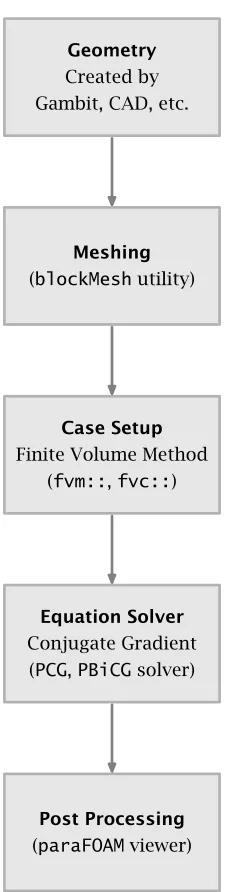
This behavior is easy to explain as shown in Figure 2.1. Traditional CFD
programs divide the space into grids and apply the Navier Stokes equation,
turbulent models, boundary conditions and so on to each grid, and then
solve the problem using Finite Difference Method, Finite Volume Method, or
Finite Element Method. The most common way to solve the Navier-Stokes
equation in industry is to use the finite volume method. Most commercial or
open source CFD codes have a finite volume solver built in, such that all the
Geometry Created by Gambit, CAD, etc.
Meshing (blockMeshutility)
Case Setup Finite Volume Method
(fvm::,fvc::)
Equation Solver Conjugate Gradient
(PCG,PBiCGsolver)
Post Processing (paraFOAMviewer)
Figure 2.1 OpenFOAM simulation workflow (All the computations are performed by CPU)
is applied. Then the program will try to solve the linear system using the
For example, Dean and Glowinski listed all the procedures it requires
to discretize the Navier-Stokes equation into several linear equations using
the finite element approach [55]. Although the process is complicated, most
operations are just one-pass scalar-vector multiplication or vector-vector
addition, which is relatively simple and requires little time. However, solving
the linear equation takes more time. Since the Navier-Stokes equation is
non-linear, although it can be written in a linearized (matrix manipulation)
fashion, both the left side and right side of the linear equation will have
unknown variables. It requires many iterations to be converged, while
each iteration is also a conjugate gradient iteration. The ADFC project
implements the Navier-Stokes solver using finite element method in C++,
and preliminary benchmarks show similar results (90 percent of the running
time is devoted to conjugate gradient method, implemented in the source
code file gradiente_conjugado.c) as of OpenFOAM [55–56].
In mathematics, the conjugate gradient method is an algorithm for the
numerical solution of particular systems of linear equations, namely those
whose matrix is symmetric and positive-definite [57]. The conjugate gradient
method is an iterative method, so it can be applied to sparse systems
that are too large to be handled by direct methods such as the Cholesky
decomposition. Such systems often arise when numerically solving partial
differential equations [58].
positive-definite matrix can be written in a small piece of code [59]. For
exam-ple, the conjugate gradient method source code in OpenFOAM, PCG.Cand
PBiCG.Cis only 200 lines each with comments, or 70 lines with comments
stripped. This helps make GPU acceleration possible.
Each step of the Conjugate Gradient method only requires one of the
following three operations [59]:
• saxbyoperation is used to compute s=ax+by;
• productoperation is used to compute the product of a sparse matrix
times a full vector;
• dot_productoperation is used to calculate the dot product of two
vec-torsx andy.
With the following three parallel operations, the conjugate gradient
method can be implemented efficiently on a multi-core GPU:
• The parallel version of saxbycreates the number of threads that equal
to the number of elements in the vector, and for each GPU thread i, it
computes si =axi+byi.
memory) as well as to increase the efficiency (reduce theO(n2) problem
into aO(n)problem). For each GPU threadi, it calculates thei-th element
of the resulting vector.
• The parallel version ofdot_productrequires simultaneously adding all
thexiyi values together in order to utilize the parallel computing power.
There is extensive research on this topic and the most mature strategy
is to utilize the parallel prefix reduce method [61].
Finally, the originalPCG.CandPBiCG.Csource code were replaced with
the newly written OpenCL parallelized OpenCLCG.C. The changed code is
hosted on Google code.
The change of the code is massive and takes a great amount of
hu-man labor because hu-many technical difficulties are encountered during the
modification:
• GPU Programming is, by nature, much more complicated than traditional
programming in nature. Most programming interfaces and instructions
are low-level, and they require knowledge of the hardware to get
max-imized performance, However, few technical details are published by
the GPU vendors. There are also few mature tools available which can
execute runtime debugging and profiling compared to traditional CPU
• OpenFOAM (and most other mature CFD codes) use C++ programming
lan-guage to abstract higher level parameters (vectors or tensors) as classes,
and use advanced C++ features (operator overloading, templates, generic
libraries) for rapid development. However, none of these features are
available in OpenCL. This procedure should convert to a clean C
im-plementation with additional utility function and glue code to convert
between C data structures and C++ classes.
• The converted C programs should be converted to GPU version. Each
iteration should be abstracted as thread, and all the variables should
be manually allocated, deallocated, copied, sent and received, in proper
place and time. After the conversion, the code is almost expanded by ten
times, and many of its parts are solely memory objects handling code.
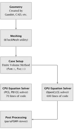
As shown in Figure 2.2, the original source code with comments purged
was about 70 lines and is now expanded to more than 600 lines, which
includes the three kernels described before as well as many important
routines for controlling the GPU to create memory allocations, performing
the calculation, as well as sending the data between GPU and CPU forward
and backward. Since all solvers and models are directly based on these
matrix solvers, the modification makes it possible to accelerate any solvers
so all the cases that were supported by the program can be simulated without
Geometry Created by Gambit, CAD, etc.
Meshing (blockMeshutility)
Case Setup Finite Volume Method
(fvm::,fvc::)
CPU Equation Solver (PCG,PBiCGsolver)
70 lines of code
GPU Equation Solver (OpenCLCGsolver)
600 lines of code
Post Processing (paraFOAMviewer)
2.4 Case studies
2.4.1 Cavity case benchmark
This research is benchmarked on an Intel Xeon CPU. The frequency of the
processor is 3.60GHz. A case is used with space divided into 500×500 grids,
and let the OpenFOAM program to simulate one time step. Different GPU
cards are used to test the program.
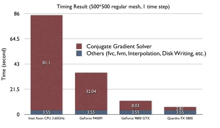
For the CPU case, this research used the unmodified OpenFOAM solver
to simulate the case. The conjugate gradient solver requires 81.1 seconds
to accomplish the work while other procedures required 3.55 seconds. This
confirms our previous statement that conjugate gradient is the bottleneck.
This research attempted to simulate the case using different GPUs with
the OpenCLCG.C solver. GeForce 9400M card uses 32.04 seconds on the
conjugate gradient procedure. GeForce 9800 GTX card uses 8.03 seconds.
Quardro FX 5800 card uses 2.81 seconds. Thereby, it is 28.86 times faster.
The performance of cards varies because each card uses different
tech-nology and configurations. For example, the Quadro card uses 512-bit
GDDR3 memory, and the memory bandwidth is two times faster than
com-rently. It is expected that with the latest generation or cards, such as Fermi,
the performance can be even further improved.
As demonstrated with the benchmark Figure 2.3, instead of using 81.1
seconds, the conjugate gradient now takes about 2.81 seconds to finish, even
faster than other procedures, which takes 3.55 seconds to finish. Thereby,
the conjugate gradient method procedure is no longer the bottleneck.
0 21.5 43 64.5 86
Intel Xeon CPU 3.60GHz GeForce 9400M GeForce 9800 GTX Quardro FX 5800
2.81 8.03
32.04 81.1
3.55 3.55
3.55 3.55
Timing Result (500*500 regular mesh, 1 time step)
Ti
me
(s
eco
nd
)
Others (fvc, fvm, Interpolation, Disk Writing, etc.) Conjugate Gradient Solver
Figure 2.3 OpenCL Benchmark for 500 by 500 regular mesh
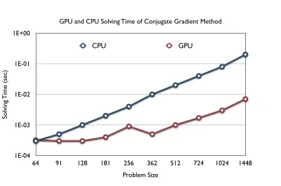
2.4.2 Pure conjugate gradient benchmark
problem size. Problems with different sizes of banded matrixes (band size
is 4) are solved by the conjugate gradient solver using Quardro FX 5800 card
and the execution times in relation to problem sizes are listed as Figure 2.4.
1E-04 1E-03 1E-02 1E-01 1E+00
64 91 128 181 256 362 512 724 1024 1448 GPU and CPU Solving Time of Conjugate Gradient Method
So
lvi
ng
Ti
me
(s
ec)
Problem Size
CPU GPU
Figure 2.4 GPU and CPU solving time of conjugate gradient method
For each single iteration, the execution time of the CPU procedure grows
linearly with the linear system problem size. This is because the number of
floating points calculation (FLOP) is a linear function of matrix and vector
sizes. However, for GPU the linear relation only holds when the problem
is because when OpenCL procedure is started, it takes some time to do
initialization, kernel compilation, data loading and pushing, etc. For small
problem sizes, GPU might be even slower than CPU, while for larger problems,
these overheads can be neglected. Not until the problem size reached
certain limits (called “turning point” in the following discussion) can the
performance grow linearly.
In Zuo’s research, the turning point is a hundred thousand while in this
research it is 256 [28–29]. This is because the two simulation procedures are
different. Zuo was executing full FFD in GPU, while this research only
per-forms a CG on GPU. FFD has only four equations that takes short simulation
time, but putting the entire program running on top of GPU requires much
more memory objects, kernels, and other resources. Thus, the initialization,
data transport, etc, take significantly longer. While in this research, the
conjugate gradient resource requirement is more light weighted, but the
actual calculation is more intense. In this case, the turning point is lower.
Although not sufficient for real time dynamic fluid simulation of large
buildings, the performance improvement has several potential applications
in building simulation. One possible area is the external coupling method of
CFD and energy simulation. With the estimated speed up presented before,
the annual case simulation is possible, and its total running time can be
reduced to within a couple of hours, comparable to the time used for Energy
2.4.3 Hot room case
The previous two cases compare the performance of conjugate gradient
alone and CFD as a whole to show speed-up over the traditional code
im-plementation. However, the accuracy of the OpenCL code is still open to
examination. To illustrate that the OpenCL enhanced version can meet
the precision requirement of building simulation study, in this case, the
originalhot room case provided by official OpenFOAM distribution is used
as testing example [62]. The performance improvement is similar (25.4x)
to the previous experiments. Here the research only focuses on numerical
precision.
In this case, a room with dimensions of 10x6x2 meters and a box that
will represent a heat source 1x1x0.5 meters in dimensions was tested. The
temperature of walls, ceiling and floor is set to 300 K and the temperature
of the heater to 500 K. The standardk-model is used and steady case is
simulated. Refer to [50] manual and case file for its setup.
After the iteration has been completed, the temperature values along
the x direction at the intersection line of plainy =0.7H and plainz=0.5D
are extracted from the result file and compared. CPU version’s result and
GPU version’s are almost the same, with relative difference lower than 0.1
difference between CPU and GPU results, however, are related to rounding
errors during the numerical evaluations.
2.5 Conclusions
As can be seen from the first case analysis, the method presented in this
research can increase the performance of CFD computation to great extent,
with much less effort than transitioning the entire code base. It is expected
that this method can be applied to many other CFD codes as well because
most CFD codes uses finite methods.
According to the second case, the turning point of this method is lower
than previous studies of GPGPU fluid simulation, which means for almost
any building simulation problem ranging from coarse grid to fine grid, GPU
is always faster.
The most important feature of the method, as can be seen from the third
case, is high precision. Its precision is of the same level as CPU calculation.
While FFD uses different equations and algorithms, this method follows the
same governing equations and numerical methods, which makes it highly
accurate and thus can be applied to research and engineering work.
It is still possible to port other portions of the source code into OpenCL
It is also possible to use preconditioned method to further optimize the
speed of conjugate gradient. However, these are beyond the scope of this
research.
This research demonstrated a way to speed up the CFD program without
Chapter 3 FFD Accelerations
3.1 Introduction
The foundation of computational fluid dynamics is based on the
Navier-Stokes equations. The Reynolds-averaged Navier-Navier-Stokes (RANS) equations
are time-averaged equations of motion for fluid flow. They are primarily
used while dealing with turbulent flows. The K-epsilon model is one of the
most common RANS turbulence models [63]. It is a two-equation model,
which means, it includes two extra transport equations to represent the
turbulent properties of the flow [64]. This allows a two-equation model to
account for history effects such as convection and diffusion of turbulent
energy. The K-epsilon model should be a reference implementation for us
since it is the most widely used solver in building science. When a new
solver is developed, the results to the K-epsilon model should be compared
to validate whether the new solver is accurate enough [65].
There are three major alternatives to the traditional method, all used
heavily in computer animation. They are the Lattice Boltzmann Method,
Smooth Particle Hydrodynamics, and Fast Fluid Dynamics.
Instead of solving the Navier-Stokes equations, the Lattice Boltzmann
such as Bhatnagar-Gross-Krook (BGK) [66–68]. Due to its particulate nature
and local dynamics, LBM has several advantages over other conventional
CFD methods, especially in dealing with complex boundaries,
incorpora-tion of microscopic interacincorpora-tions, and parallelizaincorpora-tion of the algorithm [69].
An important advantage of the Lattice Boltzmann Model allows efficient
parallelization of the simulations. Benchmark shows that LBM on parallel
machines with fast internet connection have close to linear speed-up when
more processing units are added [70–73].
In general, room airflows are not fully turbulent. Most room airflows
are locally turbulent [74]. Although measurements indicate that the flow in
the main body of ventilated rooms may be transitional, airflow at diffuser
outlets tends to be turbulent [75]. In this case, it is hard to use the Lattice
Boltzmann Method to catch the turbulent property of indoor airflow, which
is not good at simulating low Reynolds number problems.
Another alternative is Smoothed Particle Hydrodynamics (SPH). SPH was
developed by L. B. Lucy and R. A. Gingold for the simulation of astrophysical
problems, the method is general enough to be used in any kind of fluid
simulation [76–77]. J. J. Monaghan and S. A. Munzel introduce SPH in detail
[78–79] . The use of particles instead of a stationary grid simplifies these
two equations substantially. Because the number of particles is constant
There are three problems that make SPH difficult to apply to
build-ing airflow simulations. First, in order to simulate realistic chaotic fluids,
extremely high amounts of particles should be introduced to the system.
Second, there are significant difficulties when introducing the traditional
tur-bulent models into the kernel function, since turtur-bulent models usually take
advantage of time averages behavior, while simulating the particle
move-ment over a certain amount of time and taking the average behavior will
use much more computing power. Third, and most importantly, particles in
the geometry are always moving similar to the fluid. It is not possible, for
example, to calculate a steady-state case, such as the traditional one does.
This is because the traditional CFD uses Euler view and SPH uses Lagrangian
view.
The research thus will use the third approach, Fast Fluid Dynamics,
which simplifies the Navier-Stokes equation numerical solving method to
make CFD calculations faster, as the foundation. In Stam’s research, for the
first time, an unconditionally stable model which still produces complex
fluid-like flows was proposed [44]. The unconditionally stable behavior
increases the FFD model’s performance because it is possible to use arbitrary
long time step to perform the simulation. The FFD scheme was originally
proposed for computer visualization and computer games [45–46].
FFD had a successful application in computer graphics, which intends
application is open to question. Some of the recent researches apply FFD to
building simulation. Zuo and Chen validate FFD for room airflow [48–49].
Even though FFD can correctly predict the laminar flow, it has some problems
in computing turbulent flows due to the lack of turbulence treatments. Zuo
and Chen continue to make several explorations and discovered many ways
to improve their model [80–81].
The FFD algorithm is improved by increasing its speed and accuracy
[82]. Enhancement of the computing speed can be realized by modifying
the time-splitting method. Using the new FFD model for several indoor
airflows, the results show a significant reduction in computing time and great
improvements in accuracy. The method is further improved by reducing
the numerical viscosity that is caused by a linear interpolation in its
semi-Lagrangian solver [83]. The results show that the hybrid interpolation can
significantly improve the accuracy of the FFD with a small amount of extra
computing time.
In Stam’s FFD model, the simulation will almost never reach a
steady-state since the simulation numerical scheme does not ensure steady-steady-state
convergence. This research requires steady-state solution. In order to solve
this problem, the time-averaged method is reintroduced in this research.
Flows are simulated for a period of time, and averaged temperature and
A case study will be shown in the next section to validate real-time
convergence behavior of the time-averaged FFD model.
3.2 Case study
A standalone fluid simulation system is written to predict indoor air
move-ment. The system adopts Stem’s FFD algorithms. Each iteration is composed
of four computational steps [44]. After each iteration, a time-averaged
resid-ual is calculated. When the residresid-ual is below the threshold, the computation
will be halted and the solution can be treated as the steady-state solution.
The system assumes the simulated case is a 2D rectangular room
illus-trated in Figure 3.1, with one inflow vent placed on the left wall and one
outflow vent placed on the right one. The user can change the geometries
of the system. In this application, the room width and room height can be
adjusted via the interface. Also, the position of the two vents can be changed
via the slider. Finally, software users can also change inflow temperature
and speed.
The study employs fast fluid simulation algorithm developed by Jos
Stam and validated by Qinyan Chen to perform the calculation. The system
first conducts auto meshing according to the user input, then a steady case
is simulated on the fly. A vector map of the indoor air speed and a gradient
Inflow
(Temperature, Speed)
Height
Width
Outflow
positionposition
Figure 3.1 Simple Room Case Demonstration
user. Because the simulation engine is robust, the visualization is displayed
realtime just as users change the parameters.
The screenshot of the application is illustrated in Figure 3.2.
It can be seen from the software that the algorithm provides instant
response to the value change. The convergence criteria are set to meet the
averaged residual method mentioned in this chapter. The calculation is
close to real-time.
3.3 Conclusions
This chapter first analyzed the historic research of improving the simulation
performance by incorporating turbulent models. Stating those models are
Figure 3.2 Screenshot of the FluidSim program
state fluid numerical solving scheme, and Zuo and Chen’s turbulent model
for FFD.
However, although Stem’s stable fluid algorithm is unconditionally
sta-ble in terms of numerical scheme, it does not ensure steady-state solution
because of fluctuations in the fluid. By re-introducing the time-averaged
method, this research for the first time is able to simulate indoor airflow
towards steady-state solutions.
As can be seen from the case study, this solution can always give
estimated speed-up over the traditional CFD code is estimated to be 30
times to 50 times.
It is also possible to couple the FFD with GPGPU computing method
introduced in the previous chapter to increase the two performance
speed-up factors by two-fold. When multiplying the performance improvements
introduced in this and the previous chapter, it is possible to get
thousands-fold speed-up over traditional CFD code, thus making annual simulation
possible. It is estimated that for a small room with a relatively fine grid (30
by 30 by 30) ventilation simulation, it usually takes several hours to several
days to finish the annual hourly simulation, which is acceptable in some
circumstances.
To achieve more speed up over the previous improvements, good
op-timization strategies should be applied to let the simulation engine only
simulate what it needs to simulate, and reusing all the existing cases to
perform new cases results without simulation, or at least eliminates all the
unneeded iterations. In the next chapter, an optimal graph-based machine
learning algorithm is presented to demonstrate the optimal simulation
strat-egy, with the intent to further shorten the running time of annual hourly
Chapter 4 Strategy Planning Algorithm
4.1 Introduction
Since annual hourly simulations have more than 8000 hourly cases, to
calculate each case independently may take longer simulation time. It
is possible to reuse previous calculated results to generate new results,
thus considerably shortening the simulation execution time. Among many
methods, machine learning algorithms, which use existing results (training
and testing set) to train the model which is used to predict future results,
seem to be a good option.
Notably, artificial neural network (ANN) has been widely utilized. ANN
has the solid ability of self-learning and self-organization. It can employ
the prior acquired knowledge to respond to the new information rapidly
and automatically. In the area of fluid flow, the applications of the ANN
include the simulation of fluid flow and transport [84], the calculation of
coefficients of heat transfer in fluid-particle systems [85], the prediction
of flow field using a hybrid scheme of ANN [86], the dynamics simulation
of a steam generator in a nuclear reactor [87], and the computation of the
friction factor in pipeline flow [88].
An attractive attribute of machine learning models is their fast speed of
validated, it can provide almost real-time parametric and sensitivity analysis.
The typical time taken for an ANN model to execute one run is generally
several orders of magnitude smaller than that required for running a CFD
model [89]. Many researchers are trying to find a numerical method based
on ANN to solve Navier-Stokes equations [90–94]. Most of the work showed
that the trained ANN model predicts the behavior accurately. The results
demonstrate the power and robustness of ANNs for obtaining fast responses
to changing input conditions. However, although many studies focused on
using artificial neural network to solve the flow transport problem, most
researches, as listed above, do not use the Navier-Stokes equation as their
training foundation equation. Most researches have a limited focus field
such as flow and contaminant transport (GFCT) simulations, simulating Biot
number or heat transfer coefficient. Those who use Navier-Stoke equations,
usually focus on very low (less than 10) Re numbers, which are thus not
applicable to the building simulation field.
Recent studies also use meshless methods as an alternative to grid-based
flow computation [95]. Recent work has indicated that accurate results may
be obtained with meshless methods as compared with grid-based methods
[96–97]. In 2005, Zhi Shang combined ANN and meshless simulation
to-gether to simulate vapor-water two-phase flows in a tube with uniform and
non-uniform heating. It does not generate mesh in the calculation domain
chaos properties of turbulence. Moreover, some machine learning
algo-rithms would not solve the performance problems. Usually training all the
parameters requires 1,000,000 iterations, which might take a considerable
amount of time, and which takes much larger computation expanses than an
annual result simulation. Thus, indoor air is chaotic and machine learning
algorithms cannot catch the pattern very well.
CFD simulation is always time-consuming and it is even harder to cover
annual simulation (8760 static state case) in a fairly reasonable amount of
time and acceptable precision. Another way to reuse the result of existing
cases, is to use CFD to converge new case simulation using existing cases’
results as the starting point, and in some conditions the convergence will
take much fewer iterations. However, randomly using existing cases may
not achieve the desired performance gain, which is shown in the latter case
study in Section 4.2; thus, such reusing should be based on scheduling
strategies. This research will discuss a method to speed up annual CFD
simulation by using scheduling strategies. Two tools are designed in this
research to produce the optimal scheduling strategies.
1. A convergence speed predictor, discussed in Section 4.2, to predict the
number of iterations needed for using one case’s result as the starting
point to simulate the other one.
speed calculated by the predictor, to schedule an optimal strategy for
annual hourly CFD simulation by reusing previously calculated results.
4.2 Predicting the convergence speed
Though machine learning methods might not capture the chaotic property
of indoor air flow well, it can capture some of the other properties well,
such as the difference of inputs of two cases and the iteration steps needed
from one case as a string point to converge to the other case. There is a
strong relationship between the input variance and the output variance, as
well as strong relationships between the output variance and the iterations
required for convergence from one case to another. This provides the
foundation to design a convergence speed predictor used by an efficient
algorithm discussed in Section 4.3 to reuse as many existing simulated cases
as possible.
This research utilized a case study to investigate the possibility to
design a convergence speed predictor new algorithm. It is a one-room case
with a very simple ventilation system. The research used EnergyPlus to
produce annual supply air information as well as the weather information
as boundary conditions for CFD simulation. The goal of this case study
is to explore the properties and relationships of input parameters, output
10m
10m
3.5m
Inlet
Outlet
Figure 4.1 Reusable case study settings
Figure 4.1 describes the case, which has a 10mby 10m by 3.5m room. Its
location is set to Los Angeles, whose weather data will be queried and used
by the simulation. The wall has a U-value of 0.350W/m2K and the roof has
a U-value of 0.250W/m2K. The internal gains in the room are from lighting
and human body warmth. VAV box with reheat is assigned to condition the
room. The outdoor temperature (asx axis) and indoor ventilation air speed
(asy axis) of each hour from energy simulation is displayed as 8760 points
in Figure 4.2. These points served as inputs to independent CFD cases.
1. Highly condensed input distribution:
corre-0 0.15 0.30 0.45 0.60 0.75 0.90 1.05 1.20 1.35 1.50
0 10 20 30 40
Temperature (C) Air Speed (m/s)
Figure 4.2 Outdoor temperature and indoor ventilation air speed, as output by energy simulation
sponding CFD simulation. The geometry is always the same, and
bound-ary conditions are coarse and are simple functions of limited variables.
Such variables form low dimensional input space. In this example, there
are two variables (inflow air speed and outdoor temperature) and thus
two dimensional space. Complex cases will have higher dimensions, but
are usually still limited to less than five to ten dimensions.
Moreover, each dimension has very close boundaries. Building
sim-ulation has low variable variances. All temperatures fall within living
conditions for human beings. Velocities are within one or two meters
(278 K,0.45 m/s)to(308 K,1.2 m/s).
A annual simulation is composed of 8760 discrete steady state cases,
each representing an hour’s input setting in the year. There are almost
ten thousand points residing in this low dimensional, small space, which
leads to a very condensed distribution. Even if all the inputs are
distrib-uted randomly, for most of the given points, it is easy to find a point
that is very close to it. If the inputs have certain patterns similar to the
result given by this energy simulation, whose results form several
almost-horizontal lines (since the inner condition change according to a fairly
fixed schedule), such an observation can be even more obvious to find.
It is also clear that many of the cases are highly similar. For example,
if today’s noon weather is similar to tomorrow’s noon weather, chances
that indoor air control system will develop similar control strategies for
the two cases are high, not including all other uncertainties. Thus, it is
expected that the inputs of the cases are highly identical.
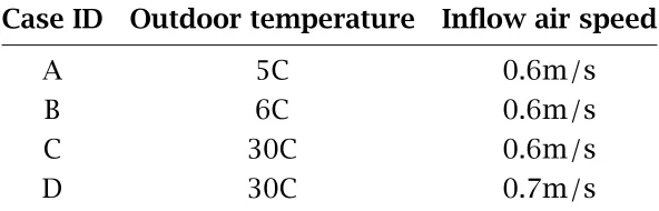
The following three observations are based on simulating four cases
randomly selected: A,B,C, andD as listed in Table 4.1.
2. Output similarity based on input similarity:
If the input variables of two CFD cases are highly similar, the
Case ID Outdoor temperature Inflow air speed
A 5C 0.6m/s
B 6C 0.6m/s
C 30C 0.6m/s
D 30C 0.7m/s
Table 4.1 Four selected cases in annual simulation
the two inputs differ, the greater the outputs deviate. For example,
case A = (5 C,0.6 m/s) and case B = (6 C,0.6 m/s) differ only by 1C,
thus their temperature field and velocity field are highly similar (less
than 1 percent difference). However, case B = (6 C,0.6 m/s) and case
C =(30 C,0.6 m/s) differs 24C, thus their outputs differ by around 10
percent. (Note: the percentage differences of temperature and velocity
field are derived by averaging the result in each grid.)
3. Input has different impact on output:
Different parameters usually have different levels of impact on the
output. Output is highly sensitive to some of the input variables.
Con-sidering the experiment, the outdoor temperature does not affect the
indoor airflow too much while the slightest change in inflow velocity has
a great impact on final results. For example, case B = (6 C,0.6 m/s)
and case C = (30 C,0.6 m/s) differ around 10 percent. However, case
outdoor temperature.
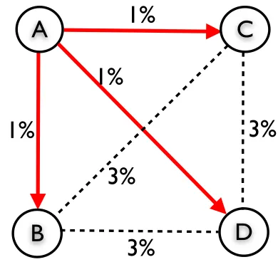
4. Iterations depend on output similarities:
Usually the number of iterations needed for using caseA’s result as
the starting point to simulate B, heavily depends on whether case A’s
result is similar to B’s result or not. This property is easy to explain.
When using caseA’s result as the initial starting point and to start the
conjugate gradient method iteration, the converging speed from Ato B
is closely related to their solution distance.
In this example, each case takes roughly 2000 iterations to
con-verge without basing them on any pre-calculated result as a starting
point. However, if two case’s outputs are similar, it requires fewer
it-erations. As described before, since case A = (5 C,0.6 m/s) and case
B =(6 C,0.6 m/s)are highly similar (less than 1 percent difference), It
takes just 22 steps to complete the B case simulation when using A’s
result as the starting point. On the contrary, according to a previous
analysis, case C = (30 C,0.6 m/s) and case D = (30 C,0.7 m/s) differ
greatly (greater than 50 percent difference). While using case C’s result
as the starting point to converge to caseD, it takes 2145 iteration steps,
almost the same iteration steps required for simulation without the bases
of existing results. CaseB and caseC’s similarity lies in between (around
10 percent difference), and it takes 364 steps fromB to C. Thus,
(such as usingC to simulateD) may not be favorable, and can even hurt
the performance. One should always choose the optimal starting existing
case for each of the case.
Cases Input Difference Output Difference Iterations
A-B (1C, 0m/s) 1 percent 22
B-C (24C, 0m/s) 10 percent 364
C-D (0C, 0.1m/s) 50 percent 2145
Table 4.2 Summary of relationship between input difference and iterations needed to converge from one case to another
The results of the previous three observations are summarized Table 4.2.
The results reveal that the three quantities (input difference of two cases,
output difference of two cases, and the number of iterations needed for
using one case’s result as a starting point to simulate the other one) are
inherently equivalent. Thus,the output difference can be used as an indicator
of convergence speed.
From the four observations in the case study, the following conclusions
can be drawn:
1. Case reusing is possible since many cases are similar, according to the
first observation.
with input difference and iteration steps needed, via the linkage of their
output difference, rather than simply using the input-output pair as a
testing and training set.
The two findings reveal that although it is difficult to generate a model
to formulate the case output as a function of case input, it is much easier
to formulate the difference of case outputs as a function of the difference
of case inputs. Thus, rather than training using the input and output data,
in this research, the difference of the inputs and the difference of the
outputs are used as training set and testing set. Moreover, according to the
observations above, the predicted difference’s magnitude can be used as a
strong indicator of the convergence speed.
Based on the machine learning model, a new scheduling algorithm will
be developed. The following section describes the algorithm structure in
its details to speed up by reusing as many existing cases as possible.
4.3 Minimal simulation by case reuse
There are large amount of similar cases for annual simulation. The output
similarities of cases can be directly predicted by the input similarities. Then
the optimal simulation strategies, which yields the list of simulation ordering
to ensure the fastest converging speed between every two nearby cases, will