Volume 2009, Article ID 381673,10pages doi:10.1155/2009/381673
Research Article
A Robust Subpixel Motion Estimation Algorithm Using
HOS in the Parametric Domain
E. M. Ismaili Aalaoui,
1, 2E. Ibn-Elhaj,
2and E. H. Bouyakhf
11Facult´e des Sciences de Rabat, Universit´e Mohammed V Agdal, 4 avenue Ibn Battouta, B.P. 1014 RP, 10000 Rabat, Morocco 2Department of Telecommunication, Institut National des Postes et T´el´ecommunication, avenue Allal Al Fassi,
Madinat El Irfane, 10000 Rabat, Morocco
Correspondence should be addressed to E. M. Ismaili Aalaoui,[email protected]
Received 28 April 2008; Accepted 24 October 2008
Recommended by Simon Lucey
Motion estimation techniques are widely used in todays video processing systems. The most frequently used techniques are the optical flow method and phase correlation method. The vast majority of these algorithms consider noise-free data. Thus, in the case of the image sequences are severely corrupted by additive Gaussian (perhaps non-Gaussian) noises of unknown covariance, the classical techniques will fail to work because they will also estimate the noise spatial correlation. In this paper, we have studied this topic from a viewpoint different from the above to explore the fundamental limits in image motion estimation. Our scheme is based on subpixel motion estimation algorithm using bispectrum in the parametric domain. The motion vector of a moving object is estimated by solving linear equations involving third-order hologram and the matrix containing Dirac delta function. Simulation results are presented and compared to the optical flow and phase correlation algorithms; this approach provides more reliable displacement estimates particularly for complex noisy image sequences. In our simulation, we used the database freely available on the web.
Copyright © 2009 E. M. Ismaili Aalaoui et al. This is an open access article distributed under the Creative Commons Attribution License, which permits unrestricted use, distribution, and reproduction in any medium, provided the original work is properly cited.
1. Introduction
The importance of image sequence processing is constantly growing with the ever increasing use of television and video systems in consumer, commercial, medical, and scientific applications. Image sequences can be acquired by film-based motion picture cameras or electronic video cameras. In either case, there are several factors related to imaging sensor limitations that contribute to the graininess (noise) of resulting images. Electronic sensor noise and film grain are among these factors [1]. In many cases, graininess may result in visually disturbing degradation of the image quality, or it may mask important image information. Even if the noise may not be perceived at full-speed video due to the temporal
masking effect of the eye, it often leads to unacceptable
single-frame hardcopies and to poor-quality freeze-frames
that adversely affect the performance of subsequent image
analysis [2].
The motion estimation process must be able to track objects within a noisy source. In a noisy source, objects appear to change from frame to frame because of the noise, not necessarily as the result of object motion [3].
Tracking objects within a noisy environment is difficult,
especially if the image frames are severely corrupted by additive Gaussian noises of unknown covariance; second-order statistics methods do not work well.
Higher-order statistics (HOS) in general and the bis-pectrum (order 3) in particular have recently been widely used as an important tool for signal processing. The classical methods based on the power spectrum are now being
effectively superseded by the bispectral ones due to some
definite disadvantages of the former. These include the inability to identify systems fed by non-Gaussian noise (NGN) inputs and nonminimum phase (NMP) systems and identification of system nonlinearity [4]. In these cases, the
these, the identifiability of NMP systems has received the maximum attention from researchers.
HOS-based methods have been proposed to estimate motion between image frames [5–9]. In, the motion esti-mation is based on the bispectrum method for sub-pixel resolution of noisy image sequences. In [7], the displacement vector is obtained by maximizing a third-order statistics cri-terion. In [8], the global motion parameters are obtained by a new region recursive algorithm. In [6], several algorithms are developed based on a parametric cumulant method, a cumulant-matching method, and a mean kurtosis error criterion. The latter is an extension of the quadratic pixel-recursive method by Netravali and Robbins [10]. In [11], it is shown that such statistical parameters are insensitive to addi-tive Gaussian noises. In particular, bispectrum parameters are insensitive to any symmetrically distributed noise and also exhibit the capability of better characterizing NGN and identifying NMP linear systems as well as nonlinear systems. Therefore, transformation to a higher-order domain reduces the effect of noise significantly. In this correspondence, a novel algorithm for the detection of motion vectors in video sequences is proposed. The algorithm uses bispectrum model-based subpixel motion estimation in the parametric domain for noisy image sequences to obtain a measure of content similarity for temporally adjacent frames and responds very well to scene motion vectors. The algorithm is insensitive to the presence of symmetrically distributed noise.
The outline of this paper is as follows. First, the problem formulation is introduced inSection 2. InSection 3, we first present briefly the definitions and properties of the bis-pecrum and cross-bispectrum. Next, we describe the motion estimation in the parametric domain. High-accuracy sub-pixel motion estimation is discussed inSection 4.Section 5
presents an evaluation of the computational complexity of our algorithm. The results of the experimental evaluation of
the proposed method are shown inSection 6and compared
to existing methods whileSection 7concludes the paper.
2. Problem Formulation
The problem of motion estimation can be stated as follows: “Given an image sequence, compute a representation of the motion field that best aligns pixels in one frame of the sequence with those in the next” [9]. This is formulated as follows:
gk−1(x,y)= fk−1(x,y) +nk−1(x,y), (1)
gk(x,y)= fk(x,y) +nk(x,y)
= fk−1
x−dx,y−dy
+nk(x,y), (2)
where (x,y) denotes spatial image position of a point;
gk(x,y) and gk−1(x,y) are observed image intensities at instants k and k −1, respectively; fk(x,y) and fk−1(x,y) are noise-free frames; nk(x,y) and nk−1(x,y) are assumed to be spatially and temporally stationary, zero-mean image Gaussian (or non-Gaussian) noise sequences with unknown
s1 r1
r2 s2
Figure1: Physical representation of cumulants [4].
covariance; and (dx,dy) is the displacement vector of the object during the time interval [k−1,k].
The goal is to estimate (dx,dy) from gk(x,y) and
gk−1(x,y).
3. Bispectrum-Based Image Motion Estimation
3.1. Definitions and Properties. In this subsection, some HOS functions are defined and their properties are described in order to provide the necessary tools to understand the motion estimation methodology.
Also, the third-order autocumulant/moment sequence,
Cgkgkgk
3 (r1,r2;s1,s2), ofgk(x,y) is defined as follows [5]:
Cgkgkgk
3
r1,r2;s1,s2
=Egk(x,y)gk
x+r1,y+r2
gk
x+s1,y+s2
, (3)
whereE{·}denotes the expectation operation; (r1,r2) and (s1,s2) are two shifted versions of thegk(x,y).
To understand the theory of triple correlations physically for 2D data [4], the reader is referred toFigure 1. The Figure shows the spaces occupied by the original data (denoted by continuous box) and two shifted versions of the same data (denoted by dashed boxes). The shifts are made by the amounts (r1,r2) and (s1,s2), respectively. It is now obvious that the product of the overlapping data positions (shown by the shaded portion) denotes the triple correlation function as defined by (3).
Also, the third-order autocumulant/moment sequence is defined as follows [12]:
Cgkgkgk
3
r1,r2;s1,s2
=Cfkfkfk
3
r1,r2;s1,s2
+Cnknknk
3
r1,r2;s1,s2
.
(4)
Equation (4) states that the triple correlation of fk(x,y) plusnk(x,y) is equal to the triple correlation of the fk(x,y) plus the triple correlation of the noise. Fornk(x,y)a zero-mean Gaussian noise, then its triple correlation is identically zero [7,12]. This provides a theoretical basis for using the triple correlation (or the bispectrum) as a method of reducing the effects of additive noise. Then the termCnknknk
3 (r1,r2;s1,s2) is negligible which renders the triple correlation very effective in detecting a signal embedded in noise. Therefore,
Cgkgkgk
3
r1,r2;s1,s2
=Cfkfkfk
3
r1,r2;s1,s2
Also, nk(x,y) can be non-Gaussian if it is independent and identically distributed (i.i.d.) and nonskewed (e.g., symmetrically distributed).
The bispectrum, Bgkgkgk
3 (u1,u2;v1,v2), is defined as the 4D Fourier transform of the third-order autocumulant (or moment) [4]:
Bgkgkgk
3
u1,u2;v1,v2
=F4Cgkgkgk
3
r1,r2;s1,s2
=F4Cfkfkfk
3
r1,r2;s1,s2
=Bfkfkfk
3
u1,u2;v1,v2
,
(6)
where F4 denotes the 4D Fourier transform operation;
(u1,u2) and (v1,v2) are the frequency coordinates for the 2D Fourier transform.
LetGgk(u) be the discrete Fourier transform (DFT) of
the frame gk(x,y). Each component of the bispectrum is estimated by a triple product of Fourier coefficients as follows [12]:
Bgkgkgk
3
u1,u2;v1,v2
=Ggk
u1,u2
Ggk
v1,v2
G∗gk
u1+v1,u2+v2
, (7)
where∗indicates the complex conjugate.
The cross-bispectrum is obtained in a similar manner as the bispectrum. Thus,
Bgk−1gkgk−1 3
u1,u2;v1,v2
=Bgk−1gk−1gk−1 3
u1,u2;v1,v2
e−j2π(u1dx+u2dy),
Bgk−1gkgk−1 3
u1,u2;v1,v2
=Ggk−1
u1,u2
Ggk
v1,v2
G∗gk−1
u1+v1,u2+v2
.
(8)
On close observation and after certain algebraic
manip-ulations, (3) shows the third-order cumulant sequence to
possess the following symmetry properties [4]:
Cgkgkgk
3
r1,r2;s1,s2
=Cgkgkgk
3
s1,s2;r1,r2
=Cgkgkgk
3
−s1,−s2;r1−s1,r2−s2
=Cgkgkgk
3
s1−r1,s2−r2;−r1,−r2
=Cgkgkgk
3
r1−s1,r2−s2;−s1,−s2
=Cgkgkgk
3
−r1,−r2;s1−r1,s2−r2
.
(9)
This directly leads to the following symmetry properties of the bispectrum sequence [4]:
Bgkgkgk
3
u1,u2;v1,v2
=Bgkgkgk
3
v1,v2;u1,u2
=B∗gkgkgk
3
−v1,−v2;−u1,−u2
=B∗gkgkgk
3
−u1,−u2;−v1,−v2
=Bgkgkgk
3
−u1−v1,−u2−v2;v1,v2
=Bgkgkgk
3
u1,u2;−u1−v1,−u2−v2
=Bgkgkgk
3
−u1−v1,−u2−v2;u1,u2
=Bgkgkgk
3
v1,v2;−u1−v1,−u2−v2
.
(10)
These symmetry properties reduce the computational burden while calculating the bispectrum.
3.2. Parametric Model-Based Motion Estimation. The prob-lem of signal processing using bispectrum in the parametric domain has recently been widely addressed by researchers. Two primary schools of thought exist for this. The first
line is headed by Raghuveer and Nikias [13], who have
parametrized the bispectrum through solution of a cumulant matrix equation. The other school of thought headed
by Giannakis [14] calculates the system impulse response
coefficients directly using a linear combination of cumulant slices. Other papers have been subsequently published which give extensions and applications of these basic approaches
(see [15] and references therein). Here, we propose the
bispectrum model-based subpixel motion estimation in the parametric domain. Simulations demonstrate that this method requires large blocks of data and thus may be appro-priate for estimating object displacement in background noise. Consequently, our approach will be derived in this context and hence, (dx,dy)=const. in (2). Substituting fk−1 from (1) into (2) we obtain
gk(x,y)=
i∈R
j∈R
α(i,j)gk−1(x−i,y−j)
+nk(x,y) +nk−1
x−dx,y−dy
,
(11)
where, in theory, α(i,j) = 0 for all{(i,j)}except (i,j) =
(dx,dy), andα(dx,dy)= 1. If the search regionRcontains the largest possible horizontal and vertical delays, and if we takegk(x,y) forgk(x+r1,y+r2), we obtain
gk
x+r1,y+r2
=
i∈R
j∈R
α(i,j)gk−1
x−i+r1,y−j+r2
+nk
x+r1,y+r2
+nk−1
x+r1−dx,y+r2−dy
.
(12)
By multiplying both sides of (12) bygk−1(x,y)gk−1(x+s1,y+
s2) and taking expectations, we obtain
Egk−1(x,y)gk
x+r1,y+r2
gk−1
x+s1,y+s2
=
i∈R
j∈R
α(i,j)Egk−1(x,y)gk−1
x−i+r1,y−j+r2
×gk−1
x+s1,y+s2
+Egk−1(x,y)nk
x+r1,y+r2
×gk−1
x+s1,y+s2
+Egk−1(x,y)gk−1
x+s1,y+s2
×nk−1
x+r1−dx,y+r2−dy
.
Therefore,
Cgk−1gkgk−1 3
r1,r2;s1,s2
=
i∈R
j∈R
α(i,j)Cgk−1gk−1gk−1 3
r1−i,r2−j;s1,s2
+Cgk−1nkgk−1 3
r1,r2;s1,s2
+Cgk−1nk−1gk−1 3
r1−dx,r2−dy;s1,s2
.
(14)
However,Cgk−1nkgk−1
3 (r1,r2;s1,s2) andC3gk−1nk−1gk−1(r1−dx,r2−
dy;s1,s2) are identically zero for all (r1,r2;s1,s2) due to the fact that the signal and noise are zero-mean and independent. Consequently, (14) becomes
Cgk−1gkgk−1 3
r1,r2;s1,s2
=
i∈R
j∈R
α(i,j)Cgk−1gk−1gk−1 3
r1−i,r2−j;s1,s2
.
(15)
Taking the 4D Fourier transform of (15) and rearranging, the following pulse transfer function for the system is obtained:
Bgk−1gkgk−1 3
u1,u2;v1,v2
=Bgk−1gk−1gk−1 3
u1,u2;v1,v2
i∈R
j∈R
α(i,j)e−j2π(u1i+u2j).
(16)
The third-order hologram,h(r1,r2), is then defined by
hr1,r2
=F−4
Bgk−1gkgk−1 3
u1,u2;v1,v2
Bgk−1gk−1gk−1 3
u1,u2;v1,v2
=
i∈R
j∈R
α(i,j)δr1−i,r2−j
,
(17)
where F−4 denotes the 4D inverse Fourier transform
operation.
Selecting various integers for r1 and r2, we form an overdetermined system of equations. For example, if the chosen search regionRis a rectangular that varies from−Px toPxin the horizontal direction and−PytoPyin the vertical direction , and ifr1 ranges from−Px to Px, andr2 ranges from−PytoPy, a set of linear equations can be produced as follows:
h=αδ, (18)
where
h=hl
−Px,−Py
,hl
−Px+ 1,−Py+ 1
,. . .,hl
Px,Py T
,
α=[α−Px,−Py),α
−Px+ 1,−Py+ 1
,. . .,αPx,Py T , δ= ⎡ ⎢ ⎢ ⎢ ⎢ ⎢ ⎢ ⎣
δ(0, 0) · · · δ−2Px,−2Py
δ(1, 1) · · · δ−2Px+ 1,−2Py+ 1
..
. ...
δ(2Px, 2Py) · · · δ(0, 0)
⎤ ⎥ ⎥ ⎥ ⎥ ⎥ ⎥ ⎦ . (19) 450 400 350 300 250 200 150 100 50 0
0 100 200 300 400 500 600
(a) 450 400 350 300 250 200 150 100 50 0
0 100 200 300 400 500 600
(b) 450 400 350 300 250 200 150 100 50 0
0 100 200 300 400 500 600
(c)
Figure2: Motion vector fields ofGrovesequence in the presence of noise using (a) our algorithm, (b) optical flow algorithm, (c) phase correlation algorithm.
The least-squares solution of (18) is given:
αls=
450 400 350 300 250 200 150 100 50 0
0 100 200 300 400 500 600
(a)
450 400 350 300 250 200 150 100 50 0
0 100 200 300 400 500 600
(b)
450 400 350 300 250 200 150 100 50 0
0 100 200 300 400 500 600
(c)
Figure3: Motion vector fields ofWalkingsequence in the presence of noise using (a) our algorithm, (b) optical flow algorithm, (c) phase correlation algorithm.
The least-squares solutionαls is obtained and its maximum
α(dx,dy) is determined. The image motion estimate is then (dx,dy).
Although we assume that the signals are non-Gaussian, it can be shown that for binary, deterministic signals and large
350 300 250 200 150 100 50 0
0 100 200 300 400 500
(a)
350 300 250 200 150 100 50 0
0 100 200 300 400 500
(b)
350 300 250 200 150 100 50 0
0 100 200 300 400 500
(c)
Figure4: Motion vector fields ofMequonsequence in the presence of noise using (a) our algorithm, (b) optical flow algorithm, (c) phase correlation algorithm.
images sizes bispectrum is insensitive to Gaussian noise, and thus (20) is approximately true. Therefore,
hr1,r2
=αdx,dy
δr1−dx,r2−dy
=δr1−dx,r2−dy
.
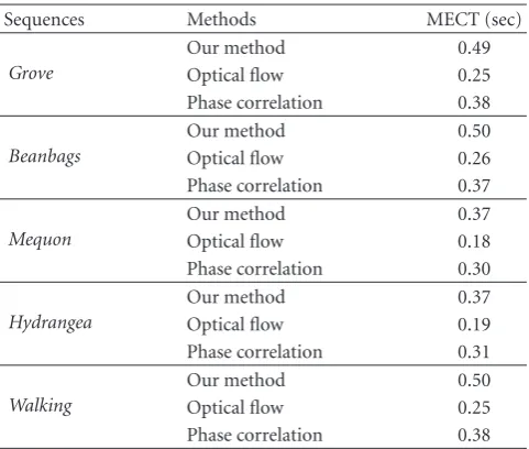
Table1: The comparison between three methods for the computa-tion time.
Sequences Methods MECT (sec)
Grove
Our method 0.49
Optical flow 0.25 Phase correlation 0.38
Beanbags
Our method 0.50
Optical flow 0.26 Phase correlation 0.37
Mequon
Our method 0.37
Optical flow 0.18 Phase correlation 0.30
Hydrangea
Our method 0.37
Optical flow 0.19 Phase correlation 0.31
Walking
Our method 0.50
Optical flow 0.25 Phase correlation 0.38
4. High-Accuracy Subpixel Motion Estimation
Subpixel performance is a critical element of the proposed algorithm. With reference to our previously published
work [16,17], we are introducing a number of important
new features, which improve the accuracy of the motion estimates.
The coordinates (r1m,r2m) of the maximum of the real-valued array h(r1,r2) can be used as an estimate of the horizontal and vertical components of motion between
gk(x,y) andgk−1(x,y) as follows:
r1m,r2m
=arg max Re hr1,r2
, (22)
where Re{·}denotes the real part of complex arrayh(r1,r2). Subpixel accuracy of motion measurements is obtained by variable-separable fitting performed in the neighborhood of the maximum using one-dimensional quadratic function. Using the notation in (22), prototype functions are fitted to the triplets:
hr1m−1,r2m
,hr1m,r2m
,hr1m+ 1,r2m
, (23)
hr1m,r2m−1
,hr1m,r2m
,hr1m,r2m+ 1
, (24)
that is, the maximum peak of the phase correlation surface and its two neighboring values on either side, vertically and horizontally.
The location of the maximum of the fitted function provides the required subpixel motion estimate (d kx, dky). Fitting a parabolic function horizontally to the data triplet (23) yields a closed-form solution for the horizontal compo-nent of the motion estimate dkxas follows:
dkx=
hr1m+ 1,r2m
−hr1m−1,r2m
2H , (25)
whereH=[h(r1m+ 1,r2m)−2h(r1m,r2m) +h(r1m−1,r2m)]. The fractional part dkyof the vertical component can be obtained in a similar way using (24) instead of (23).
Finally the horizontal and vertical components of the subpixel accurate motion estimate are obtained by comput-ing the location of the maxima of each of the above fitted quadratics.
In [18], it is shown that half-pixel accuracy motion vec-tors lead to a very significant improvement when compared to one pixel accuracy, whereas a higher precision results in negligible changes. Therefore, a half-pixel accuracy was chosen in our simulations.
5. Computational Cost Comparison
The majority of the computational cost of the proposed bispectrum is due to the fast Fourier transform (FFT). Therefore, the fundamental computation required for
bis-pectral estimates is given by (7), the triple product of
the three individual Fourier transformations, while this computation is straightforward, limitations on computer time and statistical variance impose severe limitations on
implementation of the definition of the bispectrum [19].
On the other hand, we take advantage of the symmetrical properties of the bispectrum to reduce the computational complexity and memory requirements of calculating third-order statistics. It can now be calculated in any one sector and mapped onto the others [20].
The phase correlation is estimated by multiplying each coefficient Ggk(u1,u2) by its complex conjugate, but each
component of the bispectrum is estimated by a triple product of Fourier coefficients as demonstrated in (7). Thus, the number of operations required to compute the bispectrum is significantly increased relative to the phase correlation. There
areN2/8 independent components of the bispectrum while
there are only N/2 independent components of the phase
correlation for anN×Nimage [21].
6. Simulation Results
Our experiments have aimed at evaluating the perfor-mance of the proposed approach and comparing it with that of the optical flow and phase correlation techniques. For the optical flow method we used the
implementa-tion obtained from Bruhn method [22]. In our
simula-tion we used the database freely available on the web at http://vision.middlebury.edu/flow/. We contribute three types of data to test different aspects of all techniques: real sequences of independent motion; realistic synthetic sequences; and high frame-rate video. These sequences have been chosen for their difficult motion and their different characteristics. Although the original sequences are in color, only the luminance component is used to estimate the motion vectors.
450 400 350 300 250 200 150 100 50 0
0 100 200 300 400 500 600
(a)
450 400 350 300 250 200 150 100 50 0
0 100 200 300 400 500 600
(b)
450 400 350 300 250 200 150 100 50 0
0 100 200 300 400 500 600
(c)
450 400 350 300 250 200 150 100 50 0
0 100 200 300 400 500 600
(d)
Figure5: Prediction for frame 5 of theBeanbagssequence in the presence of noise using (b) our algorithm, (c) optical flow algorithm, (d) phase correlation algorithm, (a) is original image.
half-pixel accuracy. The motion vectors estimated between
frames 6 and 7 are shown for the Grove sequence. For
this particular sequence, our scheme provides the most consistent and reliable motion vector field. Both optical flow and phase correlation algorithms fail to detect the
true motion vector. Similar results are shown in Figures3
and 4 for the motion vectors estimated between frames 2
and 3, and between frames 5 and 6 in the Walking and
Mequonsequences, respectively. Both optical flow and phase correlation algorithms produce abrupt motion vector fields. Although these abrupt motion vectors may lead to lower numerical mean squared errors (MSEs), they are incorrect motion vectors. Because of the noise resistant property of the parametric bispectrum method, it produces more reliable estimates. Therefore, our approach motion estimation results globally in motion fields more representative of the true motion in the scene.
To see more clearly the correctness of motion estimation,
we useBeanbagssequence as an example. The motion
com-pensated pictures using three methods are shown inFigure 5.
Portions of these three pictures are enlarged inFigure 6to show the differences. We observe better compensated images by the proposed method. We also observe that the motion compensated images for our scheme are much closer to the original images. Thus, the scheme is able to measure the motion vector more accurately and is more robust in general. Overall, parametric bispectrum scheme typically offers better visual quality images than the other methods.
The detection of motion vectors relies on successive phase correlation operations applied to pairs of consecutive block partitioned frames of a video sequence. The heights of the dominant peaks are monitored, and when a sudden magnitude change is detected, then this is interpreted as
a displacement vector.Figure 7shows sample phase
corre-lation surface between two blocks bk−1(x,y) and bk(x,y),
related to frames 3 and 4 of the Hydrangea sequence,
450 400 350 300 250 200 150 100 50
100 200 300 400
(a)
450 400 350 300 250 200 150 100 50
100 200 300 400
(b)
450 400 350 300 250 200 150 100 50
100 200 300 400
(c)
Figure 6: Enlarged portions of the motion compensated pictures of theBeanbags sequence using (a) our algorithm, (b) optical flow algorithm, (c) phase correlation algorithm.
the bispectrum minimizes the influence of the noise and simplifies the identification of the dominant peak on the correlation surface.
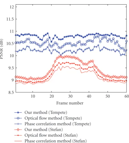
The PSNR of motion compensated is a popular per-formance measure for motion estimation, giving insight about the quality of the prediction. The PSNRs of the three
motion estimation algorithms are shown in Figure 8. This
result is obtained by using two real video sequencesTempete
andStefan. These sequences were run for 60 frames with a frame rate of 30 frame/sec. Both sequences are degraded with
additive zero-mean Gaussian noise to a signal-to-noise ratio (SNR) of 10 dB. Here we define
SNR=10 log10σ 2
f
σ2
n
, (26)
whereσ2
0 0.1 0.2 0.3 0.4 0.5 0.6 0.7 0.8 0.9
40 30
20 10
0
Ydisplac
ement
0 5 10
15 20 25 30 35
Xdisplacement
(a)
0 0.1 0.2 0.3 0.4 0.5 0.6 0.7 0.8
40 30
20 10
0
Ydisplac
ement
0 10
20 30 40
Xdisplacement
(b)
0 0.1 0.2 0.3 0.4 0.5 0.6 0.7 0.8
40 30
20 10
0
Ydisplac
ement
0 10
20 30 40
Xdisplacement
(c)
Figure7: Phase correlation surfaces between two blocks using (a) our algorithm, (b) optical flow algorithm, (c) phase correlation algorithm.
difficulty of the optical flow technique to cope with large displacement and discontinuities in the motion field. On the other hand, the normalization (equalization) operation in the phase correlation technique enhances the noise power at high frequencies, and it produces incorrect displacement estimates on noisy image sequences. On the whole, the bispectrum retains both amplitude and phase information from the Fourier transform of a signal, unlike the other techniques. This confirms the motion that the proposed
8.5 9 9.5 10 10.5 11 11.5 12
PSNR
(dB)
10 20 30 40 50 60
Frame number Our method (Tempete) Optical flow method (Tempete) Phase correlation method (Tempete) Our method (Stefan)
Optical flow method (Stefan) Phase correlation method (Stefan)
Figure8: PSNR obtained for noisy sequences (SNR=10 dB).
technique of an image is a superior feature selector utilizing the portions of the image spectrum most likely to contribute to reliable motion estimation.
In terms of complexity, this is measured by the compu-tation time. All the compucompu-tations are performed on Intel centrino duo machines (Toshiba Satellite A100-579 T5500, 2 GHz(2 CPUs)) with Windows XP. The three algorithms have been implemented using a prototype written in Matlab 6.5 R13. The comparison between three methods for the motion estimation computation time (MECT) is shown in
Table 1.
We employ 60 frames of the video Tempete sequence.
We perform the motion compensation procedure for
each current frame k with respect to reference frames
k−r, wherer = 1, 2, 3, and 4. The average PSNR of the
motion compensated images is given inTable 2, withTempete
sequence degraded with additive zero-mean Gaussian noise to an SNR of 10 dB.
The average PSNR, PSNRavg, is given as follows:
PSNRavg= 1
F
F
i=1
PSNRi, (27)
where PSNRi is the measured PSNR for frame i andF is
Table 2: Average PSNR of motion compensated images for the three motion estimation techniques (unit: dB) for Tempete
sequence.
r Our method Optical flow Phase correlation
1 10.80 10.50 10,21
2 10,23 9.83 9,59
3 9,93 9.59 9,25
4 9,68 9.24 8,81
7. Conclusion
In this paper, subpixel motion estimation algorithm using bispectrum in the parametric domain was pre-sented. We have presented a collection of datasets for the evaluation of our method, available on the web at
http://vision.middlebury.edu/flow/. In the case of the data is severely corrupted by additive Gaussian noises of unknown
covariance, our method suppresses the effects of noise
and simplifies the identification of the dominant peak on the correlation surface, unlike other techniques. At high noise levels SNR around 10 dB the optical flow and phase correlation techniques fail, yet even under these extreme conditions, the parametric bispectrum provides improve-ment in performance over the other algorithms. Overall, our scheme produces smoother displacement vector field with a
more accurate measure of object motion in different SNR
scenarios.
References
[1] N. Benmoussat, M. Faouzi Belbachir, and B. Benamar, “Motion estimation and compensation from noisy image sequences: a new filtering scheme,”Image and Vision Comput-ing, vol. 25, no. 5, pp. 686–694, 2007.
[2] J. C. Brailean, R. P. Kleihorst, S. Efstratiadis, A. K. Katsaggelos, and R. L. Lagendijk, “Noise reduction filters for dynamic image sequences: a review,”Proceedings of the IEEE, vol. 83, no. 9, pp. 1272–1292, 1995.
[3] R. M. Armitano, R. W. Schafer, F. L. Kitson, and V. Bhaskaran, “Robust block-matching motion-estimation technique for noisy sources,” inProceedings of the IEEE International Confer-ence on Acoustics, Speech, and Signal Processing (ICASSP ’97), vol. 4, pp. 2685–2688, Munich, Germany, April 1997. [4] S. Bhattacharya, N. C. Ray, and S. Sinha, “2-D signal
modelling and reconstruction using third-order cumulants,”
Signal Processing, vol. 62, no. 1, pp. 61–72, 1997.
[5] E. M. Ismaili Aalaoui and E. Ibn-Elhaj, “Estimation of subpixel motion using bispectrum,”Research Letters in Signal Processing, vol. 2008, Article ID 417915, 5 pages, 2008. [6] J. M. M. Anderson and G. B. Giannakis, “Image motion
estimation algorithms using cumulants,”IEEE Transactions on Image Processing, vol. 4, no. 3, pp. 346–357, 1995.
[7] R. P. Kleihorst, R. L. Lagendijk, and J. Biemond, “Noise reduction of severely corrupted image sequences,” in Pro-ceedings of the IEEE International Conference on Acoustics, Speech, and Signal Processing (ICASSP ’93), vol. 5, pp. 293–296, Minneapolis, Minn, USA, April 1993.
[8] E. Ibn-Elhaj, D. Aboutajdine, S. Pateux, and L. Morin, “HOS-based method of global motion estimation for noisy image sequences,”Electronics Letters, vol. 35, no. 16, pp. 1320–1322, 1999.
[9] E. Sayrol, A. Gasull, and J. R. Fonollosa, “Motion estimation using higher order statistics,”IEEE Transactions Image Process-ing, vol. 5, no. 6, pp. 1077–1084, 1996.
[10] A. N. Netravali and J. D. Robbins, “Motion-compensated television coding—part I,”Bell System Technical Journal, vol. 58, no. 3, pp. 629–668, 1979.
[11] V. Murino, C. Ottonello, and S. Pagnan, “Noisy texture classification: a higher-order statistics approach,” Pattern Recognition, vol. 31, no. 4, pp. 383–393, 1998.
[12] B. M. Sadler and G. B. Giannakis, “Shift- and rotation-invariant object reconstruction using the bispectrum,”Journal of the Optical Society of America A, vol. 9, no. 1, pp. 57–69, 1992.
[13] M. R. Raghuveer and C. L. Nikias, “Bispectrum estimation: a parametric approach,”IEEE Transactions on Acoustics, Speech and Signal Processing, vol. 33, no. 5, pp. 1213–1230, 1985. [14] G. B. Giannakis, “On the identifiability of non-Gaussian
ARMA models using cumulants,”IEEE Transactions on Auto-matic Control, vol. 35, no. 1, pp. 18–26, 1990.
[15] J. M. Mendel, “Tutorial on higher-order statistics (spectra) in signal processing and system theory: theoretical results and some applications,”Proceedings of the IEEE, vol. 79, no. 3, pp. 278–305, 1991.
[16] E. M. Ismaili Aalaoui and E. Ibn-Elhaj, “Estimation of motion fields from noisy image sequences: using generalized cross-correlation methods,” in Proceedings of the IEEE Interna-tional Conference on Signal Processing and Communications (ICSPC ’07), Dubai, UAE, November 2007.
[17] E. M. Ismaili Aalaoui and E. Ibn Elhaj, “Estimation of displace-ment vector field from noisy data using maximum likelihood estimator,” in Proceedings of the 14th IEEE International Conference on Electronics, Circuits, and Systems (ICECS ’07), pp. 1380–1383, Marrakech, Morocco, December 2007. [18] G. Madec, “Half pixel accuracy in block matching,” in
Proceed-ings on the Picture Coding Symposium (PCS ’90), Cambridge, Mass, USA, March 1990.
[19] K. S. Lii and K. N. Helland, “Cross-bispectrum computation and variance estimation,”ACM Transactions on Mathematical Software, vol. 7, no. 3, pp. 284–294, 1981.
[20] J.-M. Le Caillec and R. Garello, “Comparison of statistical indices using third order statistics for nonlinearity detection,”
Signal Processing, vol. 84, no. 3, pp. 499–525, 2004.
[21] R. W. Means, B. Wallach, and D. Busby, “Bispectrum sig-nal processing on HNC’s SIMD numerical array processor (SNAP),” in Proceedings of the ACM/IEEE Conference on Supercomputing (SC ’93), pp. 535–537, Portland, Ore, USA, November 1993.