Research on Calibration Method for the Installation
Error of three-axis Acceleration Sensor
ZHANG Hui, CHAI Wei, ZENG Huan-tao, LUO Qiang
(Research Center of Intelligent Transportation System, Sun Yat-Sen University,Guangdong Provincial Key Laboratory of Intelligent Transportation System, Guangzhou, 510006, China)
Abstract-- When three-axis acceleration sensor is used to vehicle state measurement, the effect of the installation error cannot be ignored. In order to eliminate the error, a calibration method based on mathematical model is proposed. Without any other auxiliary instruments, the calibration process can be completed by modeling measurement data from the fixed sensor. Experiments result proves the validity of this method, and the calibration error is less than 3%.
Index Term-- three-axis acceleration sensor ;installation error ;calibration
1. INTRODUCTION
In recent years, owing to the rapid development of Microelectromechanical Systems(MEMS) , acceleration sensors has been widely used in the area of automotive electronics. These applications usually need to measure acceleration data base on vehicle coordinate system, which requires every axis of acceleration sensor consistent with the one of the vehicle coordinate system[1, 2].However, due to the impact of the coarse installation process, the error between every axis of sensor and the ideal direction usually exists during measurement. The installation errors have crucial impact on measurement accuracy of the vehicle state data, so it is necessary to calibrate them.
In applications which require high-precision measurements such as aircraft, the traditional calibration methods for airborne equipment installation usually need precision measuring instruments like balance level, optical theodolite, laser radar and so on[3]. These instruments are not only high-price but also complex-operation, and to complete a calibration process is time-consuming, so it’s not suitable for low cost applications.
In order to minimize the impact of the installation error in the case of ease installation, this paper analyzes and deduces the installation error model, and then establishes the error calibration method according to Euler’s theorem. The calibration is completed only by calculating sensor self data, and the process is simple-operation and low cost without the
aid of other measuring instruments. Finally this method is proved reliable by simulation test.
2. INSTALLATION ERROR ANALYSIS
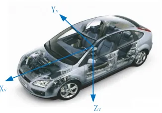
When the vehicle state measurement device based on three-axis acceleration sensor is installed on the vehicle, the ideal installation state is to make axes of three-axis accelerometer sensor parallel to the ones of the vehicle coordinate system(Figure 1) [4], in this case, measured and recorded data can reflect the true state of vehicle running. Three-axis acceleration sensor coordinate system has been calibrated at the factory, and three axes are mutually orthogonal[5].
Zv
Yv
Xv
Fig. 1. Vehicle coordinate system
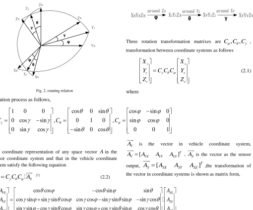
After installation, in fact it’s impossible to ensure that three axes of sensor parallel to axes of the vehicle coordinate system, the deviation between the two coordinate systems is defined as the installation error. In order to describe the installation error more intuitively, the rotation matrix is used to express the relative relationship between the two coordinate systems, and Euler angles are used to define installation error angles. According to Euler's theorem, the two space Cartesian coordinate system can completely overlap after three times rotating around the axis[6]. The rotation relationship between sensor coordinate system(
X Y Z
S S S )and the vehicleZs
Xs
Ys Zv
Z1
Yv
Y1
X1
Xv
φ
φ θ
θ γ
γ
Fig. 2. rotating relation
Rotation process as follows,
XsYsZs
X
1Y
1Zs
XvY
1Z
1XvYvZv
around Zs around Y1 around Xv
φ
θ
γ
Three rotation transformation matrixes are
C C C
,
,
, transformation between coordinate systems as followsv s
v s
v s
X
X
Y
C C C
Y
Z
Z
(2.1)
where
1
0
0
cos
0
sin
cos
sin
0
0 cos
sin
,
0
1
0
,
sin
cos
0
0
sin
cos
sin
0 cos
0
0
1
C
C
C
The coordinate representation of any space vector
A
in the sensor coordinate system and that in the vehicle coordinate system satisfy the following equationV S
A
C C C A
[7] (2.2)V
A
is the vector in vehicle coordinate system,[
]
TV VX VY VZ
A
A
A
A
,A
S is the vector as the sensoroutput,
A
S
[
A
SXA
SYA
SZ]
T ,the transformation of the vector in coordinate systems is shown as matrix form,cos cos
cos sin
sin
cos sin
sin sin cos
cos cos
sin sin sin
sin cos
sin sin
cos sin cos
sin cos
cos sin sin
cos cos
VX SX
VY SY
VZ SZ
A
A
A
A
A
A
(2.3)
Equation (2.3) indicate the transformation between the two coordinate systems, the three angles φ, θ, γ of Coefficient matrix is the installation error angle of the sensor. As long as installation error angle φ, θ, γ can be obtained, the value of acceleration in vehicle coordinate system can be calculated through equation (2.3) to overcome the impact of the installation error.
3. CALIBRATION METHOD OF INSTALLATION ERROR
The calibration of installation error is to calculate the three error angle φ、θ、γ. In the stationary state, every axis of the sensor has the output due to the gravity. As the Euler rotation relationship between the vehicle coordinate system and
geographic coordinate system, When the vehicle is stationary on a plane, the Euler matrix equation can be established through transformation of acceleration of gravity between coordinate systems[8]. And this equation is used to establish the calibration model of the error together with equation (2.3).
3.1 Calibration model
V V V
X Y Z
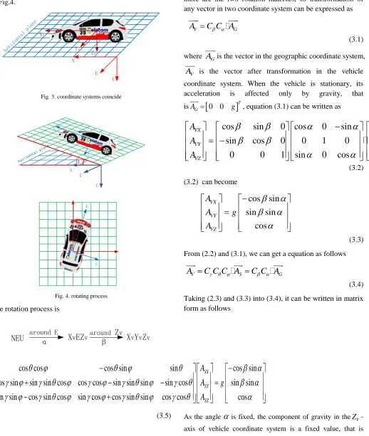
coincides exactly with the geographic coordinatesystem
NEU
(Figure 3), the twice rotation process is shown in Fig.4.Xv
Zv
hori zont
al p lane
N
U E
Yv
Fig. 3. coordinate systems coincide
Xv
Zv horizo
ntal p lane
α
NE
U
Xv
Yv β
Fig. 4. rotating process
The rotation process is
NEU
around Eα
XvEZv
around Zvβ
XvYvZv
where
is the slope angle,
is the angle between thefront direction of vehicle and the direction of max slope, there are the two rotation matrixes, so transformation of any vector in two coordinate system can be expressed as
V G
A
C C A
(3.1)
where
A
Gis the vector in the geographic coordinate system,V
A
is the vector after transformation in the vehiclecoordinate system. When the vehicle is stationary, its acceleration is affected only by gravity, that
is
A
G
0 0
g
T, equation (3.1) can be written ascos
sin
0
cos
0
sin
0
sin
cos
0
0
1
0
0
0
0
1
sin
0
cos
VX
VY
VZ
A
A
A
g
(3.2)
(3.2) can become
cos
sin
sin
sin
cos
VX
VY
VZ
A
A
g
A
(3.3)
From (2.2) and (3.1), we can get a equation as follows
V S G
A
C C C A
C C A
(3.4)
Taking (2.3) and (3.3) into (3.4), it can be written in matrix form as follows
cos cos
cos sin
sin
cos sin
cos sin
sin sin cos
cos cos
sin sin sin
sin cos
sin sin
sin sin
cos sin cos
sin cos
cos sin sin
cos cos
cos
SX
SY
SZ
A
A
g
A
(3.5) As the angle
is fixed, the component of gravity in theZ
V-cos
g
, which is not change with the angle
. From (3.5),we can obtain a equation as follows(sin sin
cos sin cos )
A
SX
(sin cos
cos sin sin )
A
SY
(cos cos )
A
SZ
g
cos
(3.6)
As
A
SX,
A
SY,
A
SZ are the measured value of components ofgravity acceleration in every axis, can be calculated from equation group through several measurements. However, due to measurement error, directly solve may lead to no solution or large error. Therefore, numerical analysis is necessary to calculate.
3.2 Installation error solution
Equation (3.6) can be written as a space plane equation
1
SX SY SZ
A A
B A
C A
(3.7)
where the parameters A B C, , can be expressed as
sin sin
cos sin cos
cos
sin cos
cos sin sin
cos
cos cos
cos
A
g
B
g
C
g
(3.8)Assuming that the outputs of three-axis acceleration sensor are coordinates of a space point, then these points distribute on this space plane.
If the space plane equation (3.7) and the slope angle is conformed, equation group (3.8) can be solved to get the installation error angle φ,θ,γ[9].
The
A B C
, ,
in space plane equation (3.7) can be solved through the least-squares fitting method, assume that there are n groups measured data of sensor,( ,
x y z
i i, ),
ii
1, 2...,
n
, and the equation of least-squares fitting for space plane is shown as follows2
2
2
1
n n n n
i i i i i i
n n n n
i i i i i i
n n n n
i i i i i i
A
B
C
x
x y
x z
x
x y
y
y z
y
x z
y z
z
z
(3.9)From (3.9), the value of
A B C
, ,
can be calculated[10]. Thevalue of also can be calculated from measured data of acceleration senor. The above-mentioned rotation relationship from sensor coordinate system to the vehicle coordinate system, (2.3) is established through the equation of Euler's theorem. Similarly make three times rotation from the vehicle coordinate system to the sensor coordinate system, three rotation angles are
, ,
,the equation isgiven by
cos cos
cos sin
sin
cos sin
sin sin cos
cos cos
sin sin sin
sin cos
sin sin
cos sin cos
sin cos
cos sin sin
cos cos
SX VX SY VY SZ VZ
A
A
A
A
A
A
(3.10) From (3.10) and (3.3) ,we can get a equation as
cos cos
cos sin
sin
cos sin
cos sin
sin sin cos
cos cos
sin sin sin
sin cos
sin sin
sin sin
cos sin cos
sin cos
cos sin sin
cos cos
cos
SX SY SZ
A
A
g
A
(3.11)( )
(
)
2 sin cos
( )
(
)
2 cos sin
cos
( )
(
)
2 cos cos
cos
SX SX
SY SY
SZ SZ
A
A
A
A
g
A
A
(3.12)
From (3.12), we obtain
2 2 2
(
( )
(
))
(
( )
(
))
(
( )
(
))
cos
2
SX SX SY SY SZ SZ
A
A
A
A
A
A
g
(3.13)
Now, the value of
can be calculated.Taking
A B C
, ,
and
into equation (3.8), we can get theinstallation error angles φ,θ,γ by solving the equation group(3.8), and the calibration of installation error is completed.
4 . VERIFICATION OF CALIBRATION METHOD
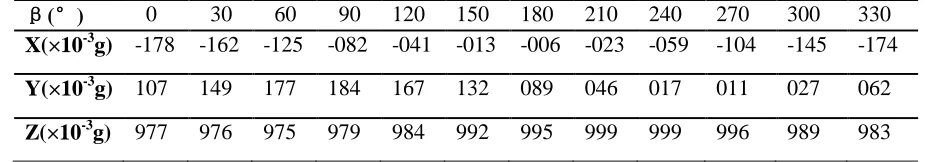
In order to verify the effectiveness of calibration method, we can test it through simulation experiment. Firstly it’s assumed that error angles γ=5°,θ=6°,φ=7°,and the slope angle
=5 ° and that the parking angle
is 0°,30°,60°,…,330°, corresponding simulation data of sensor is shown in Table I, where X,Y,Z are data of every axis. Taking static random measurement error of sensor (± 0.001g) into account, add random noise (0.001g) to the simulation data.Table I Simulation data
β
(
°
)
0
30
60
90
120
150
180
210
240
270
300
330
X(×10
-3g)
-178 -162 -125 -082 -041 -013 -006 -023 -059
-104 -145 -174
Y(×10
-3g)
107
149
177
184
167
132
089
046
017
011
027
062
Fig. 5. (a) Distribution of data points fig.5(b) Fitting Plane
The distribution of 12 sets of data points in 3D space is shown in Fig.5(a), the space plane fitted by least-squares fitting is shown in Fig.5(b), the expression of the space plane is
-0.0944x+0.1094y+0.9941z=1
(4.1)Taking the data that
is different of 180°into equation (3.13), we can get 6 sets of
. Then the average value
=5.1192° , so the relative error Er(
)=2.38%。Taking the parameters of (4.1) and into (3.8) we can get equation group as
sin sin
cos sin cos
0.0940
sin cos
cos sin sin
0.1045
cos cos
0.9901
(4.2)
Solving (4.2), we can obtain the value of error anglesγ
=5.2999°,θ=6.1020°,φ=6.8984°, the relative error of installation error angle Er=2.84%, so it can meet the need of engineering applications, and verify that the calibration method is effective.
5. CONCLUSION
In this paper, a calibration method for installation error of accelerometers is proposed which is based on mathematical model. The method only needs to park the vehicle on the plane several times without the aid of other precision instruments. And the simulation test verifies thatdeviation between results of the calibration method and the default value is less than 3% , and it’s in an acceptable range, so the calibration method is effective.
REFERENCES
[1] LUO Jian-fei, WU Zhong-cheng, SHEN Fei. Study on Measure Method of 3-axis Accelerometer of Car Based on ARM [J]. Instrument Technique and Sensor, 2010, 4(004): 87-88.
[2] YANG Hua-bo, ZHANG Shi-feng, CAI Hong. Configuration fix-error analysis and calibration for a gyro-free navigation system [J]. Journal of Chinese Inertial Technology, 2007, 15(001): 39-43. [3] HU Yu-qun, QIN Long-gang, HUANG Xiang. Mounted Position
Calibration for Airborne Equipment with Laser Radar [J]. Journal of Nanjing University of Aeronautics & Astronautics, 2010, 42(001): 112-116.
[4] MALEKI A F. Two-point calibration of a longitudinal acceleration sensor: US, 6347541B1 [P]. 2002.2.19.
[5] TAKAHASHI M, KONDO Y. Three-axis acceleration sensor variable in capacitance under application of acceleration: US, 5383364 [P]. 1995.1.24
[6] ZHANG Jin. Design and Realization of Vehicle Attitude Measurement System Based on ARM [D]; Beijing Jiaotong University, 2008.
[7] YANG Jie, SHI zhen, YUE Peng, CHENG Zi-jian. Calibration and compensation method on installation errors of accelerometer in GFSINS constituted of 3-axis accelerometer [J]. Systems Engineering and Electronics, 2011, 33(004): 869-878.
[8] KROHN A, BEIGL M, DECKER C, et al. Inexpensive and automatic calibration for acceleration sensors [J]. Ubiquitous Computing Systems, 2005, 245-58.
[9] QIN Fang-jun, XU Jiangning, FU Jun, ZHOU Hong. A Simplified Installation Error Calibration Method for Gyro-Free Inertial Navigation Systems [J]. Journal of Test and Measurement Technology, 2008, 22(002): 155-159.