Study on the Robust Wavelet Threshold
Technique for Heavy-tailed Noises
Guangfen Wei
School of Information and Electronics, Shandong Institute of Business and Technology, Yantai, P.R. China Email: [email protected]
Feng Su and Tao Jian
Research Institute of Information Fusion, Naval Aeronautical and Astronautical University, Yantai, P.R. China Email: [email protected]
Abstract— Interesting signals are often contaminated by heavy-tailed noise that has more outliers than Gaussian noise. Under the introduction of probability model for heavy-tailed noises, a robust wavelet threshold based on the minimax description length principle is derived in the ε -contaminated normal family for maximizing the entropy. The performance and their measurement criterion for the robust wavelet threshold are studied in this paper. By the proposed performance measurement criterion, several kinds of noisy signals are processed with the wavelet thresholding techniques. Compared with classical threshold based on Gaussian assumption, the robust threshold can eliminate the heavy-tailed noise better, even if the precise value of ε is unknown, which shows its robustness. The further experiment shows that soft threshold is more suitable than hard threshold for robust wavelet threshold technique. Finally, the robust threshold technique is applied to denoise the practically measured gas sensor dynamic signals. Results show its good performances.
Index Terms—heavy-tailed noise, robust wavelet threshold, soft threshold, hard threshold, signal detection
I. INTRODUCTION
Wavelet analysis has recently played a more and more important role in signal processing applications [1-3]. Many simple nonlinear thresholding filters based on wavelets have acted effectively for denoising [4-6]. Based on singularity of signals, Mallat has suppressed noise effectively in wavelet transform domain by preserving only the local maxima of the transform coefficients [7]. The noise suppression is achieved by thresholding the wavelet transform of the contaminated signal. And Donoho has derived a threshold by a minimax approach based on Gaussian noise model [8]. This thresholding technique has been applied to many areas to reduce the normally distributed white noises,
such as ECG signals and image signals [4,9].
However, in practical case, the contaminated signals such as radar, sonar echo signals and most other signals contain many noises with large magnitudes, which do not subject to Gaussian distribution, but a heavy-tailed noise model [10]. The noise is assumed to be independent and identically distributed (i.i.d) with a density which is a member of anε-contamination class for which the nominal distribution has heavier than exponential tails [11]. For heavy-tailed noise has more outliers than Gaussian noise, many methods based on Gaussian noise model cannot gain perfect effectiveness for heavy-tailed noise [12]. Thus a robust wavelet threshold method based on the minimax description length principle is derived, which determines the least favorable distribution in the ε-contaminated normal family as the member that maximizes the entropy [12]. This robust wavelet threshold technique is in detail studied including its performances, and the measurements of performances, and the application to denoise the practically measured gas sensor signals.
This paper is constructed as follows. Firstly the probability model for heavy-tailed noises and the robust wavelet threshold technique are introduced and analyzed. Then based on an appropriate effectiveness measure for removing heavy-tailed noise, the classical threshold method and the robust wavelet threshold method are compared by Monte Carlo simulation. Moreover, the soft threshold and hard threshold for robust wavelet threshold technique are also analyzed and compared. An application in gas sensor signal denoising shows the prospect of the robust wavelet threshold technique. Finally, some conclusions are given as well as the hints for future work.
II. MODEL FOR HEAVY-TAILED NOISES
Generally, the observed signals are illustrated through the additive noise model, which is given by
( ) ( ) ( )
t st ntx = + (1)
where s(t) is an unknown deterministic signal, n(t) is the zero-mean noise process, and x(t) is the observed signal.
Manuscript received November 30, 2010; revised January 30, 2011; accepted February15, 2010.
The work is supported by the NSFC project (No.60746001) and the Shandong Province Grant (BS2010DX022, ZR2010FL020).
The aim of denoising is to recover the signal s(t) from the noisy signal x(t). In order to reach this purpose, the noise process is usually supposed to subject to Gaussian distribution. Under this assumption, many methods have been proposed.
In most applications, the data are assumed to be conditionally normal, and the likelihood is therefore Gaussian. Here for heavy-tailed noises, the noise probabilistic distribution model is constructed by Huber [13]. Assuming that the noise distribution f is a scaled version of an unknown member of the family of ε -contaminated normal distribution,
(
)
{
G G F}
Pε = 1−ε Φ+ε : ∈ (2)
where Φ denotes the standard normal distribution,
F
denotes the set of all suitably smooth distribution functions, and ε∈(0,1)is the known fraction of contamination.
Krim and Shick [12] also followed this assumption and obtained same model by solving a minimax problem. They denoted that the signal estimation problem can be cast as one of location parameter estimation and the estimators can be assumed to be in the set of all integrable mappings from ℜ to ℜ. By solving a minimax problems where the entropy is maximized over all distributions in Pε, the least favorable noise distribution is found and the minimax description length(MDL) criterion for that distribution is evaluated. And the description length is minimized over all estimators in the set of all integrable mappings from ℜ to ℜ.
The least favorable noise distribution in Pε which maximizes the entropy, is precisely the same as that found by Huber to maximize the asymptotic variance: it is Gaussian in the center and Laplacian in the tails, and switches from one to the other at a point whose value depends on the fraction of contamination ε. Larger fractions corresponding to smaller switching points and vice versa. This distribution fH∈Pε that minimizes the
negentropy is obtained and defined as
( )
(
) ( )
( )( )
(
) ( )
(
) ( )
( )( )⎪ ⎩ ⎪ ⎨ ⎧
≥ −
< < − −
− ≤ −
=
+ −
+
a c e
a
a c a c
a c e
a
c f
a ac
a ac
H
, 1
, 1
, 1
2 2
2 2
/ 1
/ 1
σ σ σ
σ σ
φ ε
φ ε
φ ε
. (3)
where φσ is the normal density function with mean zero and variance σ2, and a is related to ε .
Let Φσ be the normal distribution function with mean zero. According to the symmetry of fH, the relationship
between a and ε is given by
( )
( )
ε ε σ
φ
σ σ
− = ⎟ ⎠ ⎞ ⎜
⎝
⎛ −Φ −
1 /
2 2 a
a
a (4)
The above propositions and their proofs can be found in [12].
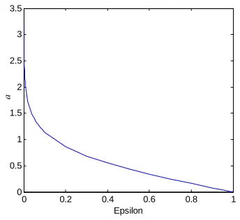
According to (4), let σ=1, the relationship between a
and ε is shown in Fig. 1. In the interval (0, 0.1), a
decreases sharply as ε increases, but in the interval (0.1, 1) the variation curve is flat. When ε→1 and a→0, the noise distribution approaches Laplacian, but when ε→0
and a→∞, the noise distribution approaches purely Gaussian.
III. ROBUST WAVELET THRESHOLD TECHNIQUE
A. The Basic Principle of Wavelet Transform
Wavelet transforms have become well known as useful tools for various signal processing applications [14]. Given a time-varying signal x(t), wavelet transforms consist of computing coefficients that are inner products of the signal and a family of “wavelets”. In a continuous wavelet transform, the wavelet corresponding to scale a and time location b is
) ( | |
1 ) (
,
a b t
a t b a
−
= ψ
ψ (5)
where
ψ
(t) is the wavelet “prototype”, which can be thought of a band-pass function. The factor 1/2|
|a − is used to ensure energy preservation.
The continuous wavelet transform (CWT) was originally introduced by Goupillaud, Grossmann, and Morlet [15]. Time t and the time-scale parameters vary continuously:
∫
= xt t dt
b a t x
CWT{ (); , } () a*b() ,
ψ . (6)
( the asterisk stands for complex conjugate).
Wavelet series coefficients are sampled CWT coefficients. There are various ways of discretizing time-scale parameters (b, a), each one yields a different type of wavelet transform. The time-scale parameters (b, a) are usually sampled on a so-called “dyadic” grid in the time-scale plane (b, a), where the dilation or scale is supposed to
a
=
2
j, the translation b is supposed tob
=
k
2
j,Z
j
∈
,k
∈
Z
. Hence the scale and translation are denoted through j and k. And the discrete wavelet transform (DWT) is defined as0 0.2 0.4 0.6 0.8 1
0 0.5 1 1.5 2 2.5 3 3.5
Epsilon
a
∫
=
x
t
t
dt
C
jk(
)
jk(
)
* ,
,
ψ
. (7)The wavelet transform is used to transform the noisy signal into wavelet domain by decomposing the noisy signal into different levels of details coefficient. And the signal could be reconstructed through the inverse wavelet transform
∑∑
∈ ∈
=
Z j k Z
k j k j
t
C
t
x
(
)
,ψ
~
,(
)
. (8)If
ψ
(t)=ψ
~(t), the wavelet basis is called orthogonal basis. Wavelet series have been popularized under the form of signal decomposition onto “orthogonal wavelets” by Meyer, Mallat, Daubechies, and other authors [16-17].k j
C
, is also called the wavelet coefficient, j, k areusually integers which show the scale and translation parameters. For signal denoising, we do not concern the j, k parameters, but the amplitude. To simplify, let the set of wavelet coefficients obtained from the observed signal be denoted by
C
N=
{
C
1x,
C
2x,
"
,
C
Nx}
. Considering the orthogonal wavelets, equation (8) is changed to∑
∈=
N i i x it
C
t
x
(
)
ψ
(
)
. (9)And the signal and noise can be expressed with an orthonormal basis:
( )
=∑
( )
i i s i t C ts ψ . (10)
( )
=∑
( )
i i n i t C tn ψ . (11)
As wavelet transform is linear, x(t) can be given by
n i s i x
i C C
C = + . (12)
Let exactly K of these coefficients contain signal information, while the remainder only contains noise. If necessary, these coefficients are reindexed as
⎩ ⎨ ⎧ + = = otherwise C K i C C C n i n i s i x i , , , 2 , 1 " ,
. (13)
By assumption, the set of noise coefficients
{ }
C
in is asample of independent and identically distributed random variates drawn from Huber’s distribution
f
H.From the above equations, if s =0 i
C for a given i, it
implies that the corresponding observation coefficients
x i
C represent “pure noise”. The wavelet denoising determines which wavelet coefficients represent signal primarily and which represent noise mainly.
B. Wavelet Threshold Denoising
Wavelet threshold denoising is based on the idea that the energy of the signal to be defined concentrates on some wavelet coefficients, while the energy of noise spreads throughout all wavelet coefficients. Similarity
between the basic wavelet and the signal to be defined plays a very important role, making it possible for the signal to concentrate on fewer coefficients. Wavelet threshold denoising is a very efficient method, the purpose of which is to remove the noises [18].
Generally, the wavelet threshold denoising procedure has the following steps [8]:
(1) Transform signal to the time-scale plane by means of a wavelet transform. It is possible to acquire the results of the wavelet coefficients on different scales.
(2) Assess the threshold and in accordance with the established rules, shrink the wavelet coefficients.
(3) Use the shrunken coefficients to carry out the inverse wavelet transform. The series recovered is the estimation of the determined signal.
The second step has a large impact upon the effectiveness of the procedure.
Thresholding is one of the important steps to remove noise. Thresholding function in this study covers hard and soft thresholding. Thresholding function is the wavelet shrinkage function which determines how the threshold is applied to wavelet coefficients. The definition of soft and hard threshold is given by [8].
The soft thresholding function is defined as
(
)
( )
(
)
⎩ ⎨ ⎧ ≤ > − = th C th C th C C th C Tsoft , 0 , sgn, . (14)
where C and th are wavelet coefficient and threshold. And the sgn(x) is the symbol function:
⎩ ⎨ ⎧ < − > = 0 , 1 0 , 1 ) sgn( x x
x . (15)
It is called thrink or kill which is an extension of hard thresholding, first setting the elements whose absolute values are lower than the threshold to zero, and then shrinking the other coefficients.
The hard thresholding function used by Donoho is:
(
)
⎩ ⎨ ⎧ ≤ > = th C th C C th C Thard , 0 ,, . (16)
where C and th are wavelet coefficient and threshold. It is called keep or kill, keep the elements whose absolute value is greater than the threshold, set the elements lower than the threshold to zero.
C. Robust Wavelet Threshold
No matter hard thresholding or soft thresholding, the determination of the threshold is most critical. According to Donoho, the universal threshold rule should be applied in the second step. The universal threshold is defined as follows:
N
th
=
σ
2
ln
. (17)finest scale wavelet coefficients, whereas N refers to the number of data samples in the measured signal. [18]
Equation (17) has been widely used as the threshold, which is quite classical. However, for heavy-tailed noises, according to fH, the robust threshold technique is obtained
as
1) When logN>a2/2σ2, the coefficients x i C will
be truncated if
N a a Cx
i log
2
2 σ +
< . (18)
2) When logN≤a2/2σ2, the coefficients x i
C
willbe truncated if
N Cx
i <σ 2log . (19)
where N denotes the length of coefficients at a given level.
The robust wavelet threshold adopts data description length as the criterion of choice for quantifying the tradeoff between noise removing and signal retaining. It can resolve the tradeoff between model complexity and goodness-of-fit well.
IV. SIMULATION RESULTS AND ANALYSIS
For comparison, the threshold defined by (17) is called as the classical threshold. Hence in the simulations, the classical threshold and the robust threshold are compared firstly. And then the sensitivity of robust threshold to ε is discussed. By comparing the results of soft threshold and hard threshold, the better one for robust wavelet threshold technique is determined. Finally, the real gas sensor’s signal is denoised with the method.
A. Signal Denoising
In simulation experiments, both the sine wave signal and square wave signal are chosen as the original signals with length 1024. The additive noise is independent identically distributed and obeys Pε with ε=0.1. Suppose that Φ~ N(0,1), A~ N(0,σ2) and the heavy-tailed noise obeys G= A3 [17]. Let σ=1.6 and SNR=8.5dB. The soft thresholding is adopted for the experiment. The db4 wavelet is chosen for decomposition in MATLAB. The decomposition layer is set 5.
Fig. 2 shows the simulated sine wave signal and the noisy signal, where S(n) and X(n) are the original signal and contaminated signal respectively. Fig. 3 shows the detected sine wave signal with classical threshold and robust threshold, where S1(n) and S2(n) are the detected
signal with classical threshold and robust threshold respectively. According to Fig. 2, compared with Gaussian noise, the heavy-tailed noise has more outliers. From Fig. 3 it can be seen that the classical threshold cannot suppress outliers in heavy-tailed noise effectively, while the robust threshold is efficient to decrease the heavy-tailed noise.
Fig. 4 shows the simulated square wave signal and the noisy signal, where S(n) and X(n) are the original signal
and contaminated signal respectively. And Fig. 5 shows the detected square wave signal with classical threshold and robust threshold, where S1(n) and S2(n) are the
detected signal with classical threshold and robust threshold respectively. It gives the same result as Fig. 2 and 3. And it can be seen that the robust wavelet threshold is robust both for narrow band signal and broad band signal.
B. Sensitivity to ε
ε is the fraction of contamination from the heavy-tailed noise, it shows the noise distribution probability. According to (4), given ε , the parameter a can be obtained and the noise distribution probability is set. Different values are set to ε and the sensitivity of proposed threshold to ε is discussed.
Assumingε=0.1, ε=0.01, ε=0.99, correspondingly a is obtained as a=1.14, a=1.95, a=0.008 respectively. Fig. 6 shows the detection results with robust threshold under different estimated values of ε, where S2(n), S3(n) and
S4(n) correspond to the exact estimation of ε=0.1,
01 . 0
=
ε and ε =0.99 respectively. Compared with S1(n),
the robust threshold can suppress outliers more effectively than the classical threshold. Although S3(n)
retains outliers near n=930, it is still better than S1(n).
0 100 200 300 400 500 600 700 800 900 1000 -5
0 5
0 100 200 300 400 500 600 700 800 900 1000 -5
0 5
S2
(n
)
S1
(n
)
Figure 3. Detected sine wave signal with classical and robust threshold
0 100 200 300 400 500 600 700 800 900 1000
-10 -5 0 5 10 15
n
X(
n
)
0 100 200 300 400 500 600 700 800 900 1000
-5 0 5
S(
n
)
Hence it can be seen that the mixture parameter ε plays little influence on the robust threshold, which shows its robustness.
C. Performance Measurement
To evaluate the accuracy of different denoising methods, the L2 norm is generally adopted as the error
criterion [18], which is defined as
N
x
x
L
N
i
i
i
ˆ
/
1
2 2
∑
=
−
=
. (20)Under this criterion, the reconstructed error of S1 and
S2 are computed and found less different. However, from
the results it can be seen that the robust threshold is better than the classical one. Therefore, the L2 norm only could
not measure the efficiency. Under this reason, the SNR (signal-to-noise ratio) enhanced (named as SNRenh) is
proposed to denote the effectiveness [19], which is defined as
1 2
SNR
SNR
SNR
enh=
−
(21)where
SNR
1andSNR
2are the SNR before and after denoising, with dB as the unit. The SNR is defined as( )
( )
( )
(
)
⎟
⎟
⎟
⎠
⎞
⎜
⎜
⎜
⎝
⎛
−
=
∑
∑
l
N l
l
N
l
S
SNR
22
10
log
10
µ
(22)where
S
( )
l
,N
( )
l
andµ
N are signal series, noise series and noise mean value respectively [20].SNRenhdenote the average level of the noises in revised
signals. Comparing to Gaussian noise, the heavy-tailed noise has more outliers. To denote the ability to suppress the outliers, the maximum error (named as Errmax) is
proposed as a measure [19]. It is defined as
( )
∑
∑
= =
=
0 01 2
0 1
2
0 max
1
)
(
'
1
Nl N
l
n
S
N
l
Err
N
Err
β
β
(23)where
N
0is the data length,Err
'
(
l
)
is the sorted errorvalues,
0
≤
β
≤
1
. The Errmax is an average relativeerror of the maximum
β
N
0 error values.For different denoising methods, the SNR enhanced (SNRenh) can denote the global effectiveness of denoising
and the maximum error (Errmax) can denote the ability to
suppress outliers in heavy-tailed noise; the combination of SNRenh and Errmax can measure the ability to suppress
heavy-tailed noise [19].
According to SNRenh and Errmax, the robust threshold is
compared with classical threshold in Fig. 7. The original
0 100 200 300 400 500 600 700 800 900 1000
-5 0 5 10 15
0 100 200 300 400 500 600 700 800 900 1000
-5 0 5 10 15
S2
(n
)
n
n
S1
(n
)
Figure 5. Detected square wave signal with classical and robust threshold
0 100 200 300 400 500 600 700 800 900 1000
-5 0 5
0 100 200 300 400 500 600 700 800 900 1000
-5 0 5
0 100 200 300 400 500 600 700 800 900 1000
-5 0 5
n
n
n
S (
n
)
4
S (
n
)
3
S (
n
)
2
Figure 6. Detected signal with robust threshold for different ε
0 100 200 300 400 500 600 700 800 900 1000
-6 -4 -2 0 2 4 6
S(
n
)
0 100 200 300 400 500 600 700 800 900 1000
-10 0 10 20
X(
n)
n n
signal is sine wave signal, and Monte Carlo simulation is used to evaluate SNRenh and Errmax of two thresholds over
a range of SNR. Where 300 experiments were conducted at each value of SNR; the soft threshold is adopted for both methods; and the solid line and dotted line denote the robust threshold and the classical threshold respectively.
According to Fig. 7, from either SNRenh or Errmax the
robust threshold performs much better than classical threshold. When SNR>8dB, SNRenh of robust threshold is
lower than that of classical threshold, because SNR of contaminated signal is too high and the number of outliers decreases in heavy-tailed noise. When the distribution of noise approaches Gaussian, the advantage of robust threshold over classical threshold vanishes. According to Errmax in Fig. 7, it is proved that two error
curves of different thresholds are nearly the same at SNR>4dB. In a word, the robust threshold outperforms the classical threshold in removing heavy-tailed noise, especially for low SNR.
D. Discussion on Soft and Hard Threshold
During the above simulations, soft thresholding technique is adopted. In order to determine the better one for robust wavelet threshold technique between soft threshold and hard threshold, SNRenh and Errmax of soft
threshold and hard threshold are compared.
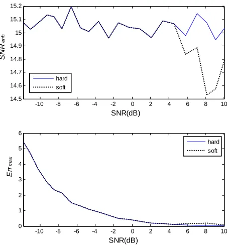
For robust threshold technique, the soft and hard thresholds are compared. The original signal is still sine wave signal, and Monte Carlo simulations with 300 experiments are conducted. SNRenh and Errmax of soft and
hard thresholds over a range of SNR are shown in Fig. 8, where the solid line and the dotted line denote soft threshold and hard threshold respectively.
In Fig. 8, according to Errmax, the soft threshold and
hard threshold are nearly the same. However, according to SNRenh, the soft threshold outperforms the hard
threshold at SNR>5dB. When the original signal is square wave signal or triangular wave signal, the same results are obtained. It is concluded that soft threshold is more suitable than hard threshold for robust wavelet threshold technique.
E. Application in Gas Sensor Signal Denoising
Semiconductor gas sensors suffer from serious shortcomings such as poor selectivity, low repeatability and response drift. In order to overcome these disadvantages, the temperature modulation technique is proposed [21-22]. By modulating the operating temperature of gas sensors, this technique has been remarkably successful in many applications. Temperature modulation alters the kinetics of the adsorption and reaction processes that take place at the sensor surface while detecting reducing or oxidizing species in the presence of atmospheric oxygen. This leads to the development of response patterns, which are characteristic of the species being detected. In other words, by retrieving information from response dynamics, new response features are obtained that confer more selectivity to metal oxide sensors.
The extraction of features from the response of chemical sensors consists in the selection of some characteristics of their temporal response sequence, which results from the interaction between sensors and the compounds to be detected. The extracted features are then input to pattern recognition systems. From a general point of view, a chemical sensor can be considered as a dynamic system whose response signal temporally evolves following, with its proper dynamics, the analytes
-10 -8 -6 -4 -2 0 2 4 6 8 10
14.5 14.6 14.7 14.8 14.9 15 15.1 15.2
SN
R
-10 -8 -6 -4 -2 0 2 4 6 8 10
0 1 2 3 4 5 6
SNR(dB)
Er
r
SNR(dB)
enh
max
hard soft hard
soft
Figure 8. SNRenh and Errmax of the soft threshold and hard threshold for
robust threshold technique -10 -8 -6 -4 -2 0 2 4 6 8
8 10 12 14 16
-10 -8 -6 -4 -2 0 2 4 6 8 0
20 40 60 80
SN
R
en
h
SNR(dB)
Er
r
ma
x
SNR(dB)
Classical Robust
Classical Robust
Figure 7. SNRenh and Errmax of the robust threshold and classical
and their concentration. Therefore, Wavelet analysis has been employed to study the properties of dynamic signals. Features could be extracted from the wavelet coefficients [23-24].
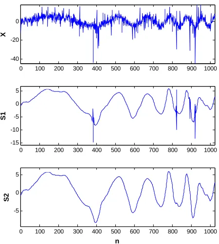
However, the real measured gas sensor signal suffers from the noises, especial the outlier noise. The upper subplot X in Fig. 9 shows a real test of modulated gas sensor signal. It can be seen that, the noise is quite the same as heavy-tailed noises discussed above. It also obeys the heavy-tailed noise probability distribution. Before extract features, the signal should be denoised. Generally used classical threshold is adopted and the result is shown in the middle subplot of Fig. 9. For the distinct outliers, it has small effects. For comparison, the robust threshold is adopted and the result is shown in the third subplot of Fig. 9. It can be seen that the noises are almost eliminated, which shows its good performances.
V. CONCLUSION
Based on the probability model for heavy-tailed noises and the wavelet denoising method, the robust wavelet threshold is studied in detail. According to an appropriate effectiveness measure for removing heavy-tailed noise, the classical Donoho threshold method and the robust wavelet threshold method are compared by Monte Carlo simulation. Following conclusions are drawn from the simulation results as following:
(1) For the heavy-tailed noise that has more outliers than Gaussian noise, the robust threshold can suppress outliers more effectively than the classical Donoho threshold.
(2) With unknown
ε
, the robust threshold can also detect signal in heavy-tailed noise, which shows its robustness.(3) The soft threshold is more suitable than the hard threshold for robust wavelet threshold technique.
(4) The robust wavelet threshold approach is effective to decrease the heavy noises from gas sensor dynamic signals. It is a quite prospective approach in signal denoising area.
However, there are still some problems need to be studied further, such as how to determine the best wavelet basis function and the optimum decomposition level. They are the further problem to be solved.
ACKNOWLEDGMENT
The authors would like to thank the financial support of National Science Foundation of China (No.60746001) and the Shandong Province Grant (No.BS2010DX022, No. ZR2010FL020).
REFERENCES
[1] S.E. El-Khamy, M.B. Al-Ghoniemy, “The wavelet
transform: a review and application to enhanced data storage reduction in mismatched filter receivers”, Thirteenth National Radio Science Conference, 1996. NRSC '96., pp.1-22, 1996.
[2] G.F. Wei, T. Jian, R.J. Qiu, “Signal denoising via median filter & wavelet shrinkage based on heavy-tailed modeling”, Proc. 8th Inter. Conf. on Signal Processing, vol.1, pp.53—55, IEEE Press, October 2006.
[3] T. Jian, Y. He, F. Su, “An algorithm analysis of median filter & wavelet threshold for heavy-tailed noise”, Signal Processing, China, vol.23, pp.79-82, 2007.
[4] H.B. Qi, X.F. Liu, C.Pan, “Discrete wavelet soft threshold denoise processing for ECG signal”, International conference on Intelligent Computation Technology and Automation, vol.1, pp.126-130, 2010.
[5] T.W. Chen, W.D. Jin, Z.X. Chen, “Feature extraction using wavelet transform for radar emitter signals”, International Conference on Communications and Mobile Computing, vol.1, pp.414-419, 2009.
[6] R. Ranta, V. Louis-Dorr, C. Heinrich, D. Wolf, “Iterative wavelet-based denoising methods and robust outlier detection”, IEEE Signal Processing Letters, vol. 12, No.8, pp. 557-560, August 2005.
[7] S. Mallat, W.L. Hwang, “Singularity detection and processing with wavelets”, IEEE Trans. on Information Theory, vol.38, pp.617-643, Dec. 1992.
[8] D.L. Donoho, “De-noising by soft-thresholding”, IEEE Trans. on Information Theory, vol.41, pp.613-627, Dec. 1995.
[9] S. G. Chang, B. Yu, M, Vetterli, “Wavelet thresholding for multiple noisy image copies”, IEEE Trans. on Image Processing, vol.9, No.9, pp. 1631-1636, September 2000. [10]T. Jian, F. Su, Y. He, “A detection algorithm of robust
neural network for heavy-tailed noise”, J. of Electronics & Information Technology, China, vol.29, pp.1864-1867, 2007.
[11]D.J. Warren, J.B. Thomas, “Asymptotically robust detection and estimation for very heavy-tailed noise”, IEEE Trans. on Information Theory, Vol.37, No.3, pp.475-481, May 1991.
0 100 200 300 400 500 600 700 800 900 1000 -40
-20 0
X
0 100 200 300 400 500 600 700 800 900 1000 -15
-10 -5 0 5
S1
0 100 200 300 400 500 600 700 800 900 1000 -5
0 5
n
S2
[12]H. Krim, I.C. Schick, “Minimax description length for signal denoising and optimized representation”, IEEE Trans. on Information Theory, vol.45, pp.898-908, 1999. [13]P. Huber, “Robust estimation of a location parameter”, Ann.
Math. Stat, vol.35, pp.1753-1758, 1964.
[14]S. Mallat, A wavelet tour of signal processing, Boston Mass Academic press, 1998.
[15]S.G. Mallat, “A theory for multiresolution signal decomposition: the wavelet representation”, IEEE Trans. on Pattern Analysis and Machine Intelligence, vol.11, Issue 7, pp.674-693, 1989.
[16]O. Rioul, P. Duhamel, “Fast algorithms for discrete and continuous wavelet transforms”, IEEE Trans. on Information Theory, vol.38, Issue 2, pp.569-586, 1992. [17]I. Djurovic, V. Katkovnik, L. Stankovic, “Instantaneous
frequency estimation based on the robust spectrogram”, IEEE Inter. Conf. on Acoustics, Speech, and Signal Processing, vol.6, pp.3517-3520, IEEE Press, 2001. [18]H.G. Zang, Z.B. Wang, Y. Zheng, “Analysis of signal
De-noising method based on an improved wavelet thresholding”, The Ninth International Conference on Electronic Measurement and Instruments, vol. 1, pp.987-990, 2009
[19]T. Jian, F. Su, D.F. Ping, “An effectiveness measure for methods of removing heavy-tailed noise”, Modern Radar, China, vol.29, pp.55-56, 79, 2007.
[20]R.H.G. Tan, V.K. Ramachandaramurthy, “Performance analysis of wavelet based denoise system for power quality disturbances”, PowerTech, 2009 IEEE Bucharest, pp.1-5, 2009.
[21]D.C.Meier, J.K.Evju, Z.Boger, B.Raman, K.D.Benksterin, C.J.Martinez, C.B.Montgomery, S.Semancik, “The potential for and ahallenges of detecting chemical hazards with temperature-programmed microsensors”, Sensors and Actuators B, vol. 121, pp.282-294, 2007.
[22]S.Nakata, H.Okunishi, Y.Nakashima, “Distinction of gases with a semiconductor sensor under a cyclic temperature modulation with second-harmonic heating”, Sensors and Actuators B, vol.119, pp.556-561, 2006.
[23]H. Ding, H.F. Ge, J.H. Liu, “High performance of gas identification by wavelet transform-based fast feature extraction from temperature modulated semiconductor gas sensors”, Sensors and Actuators B, vol.107, No.1, pp.749-755, 2005.
[24]R. Ionescu, E. Llobet, “Wavelet transform-based fast feature extraction from temperature modulated semiconductor gas sensors”, Sensors and Actuators B, vol.81, No.1, pp.289-295, 2002.
Guangfen Wei, was born at Weifang, Shandong Province of China in 1978.
She has received her B.E. in electronic engineering from Shandong Normal University in 1999, and her Ph.D in Department of Electronic Engineering, Dalian University of Technology, PR China in 2006. She has worked as post doc in Dalian University of Technology from 2006 to 2009. She works now as the associate professor in School of Information and Electronics, Shandong Institute of Business and Technology. She is a visiting scholar of Shandong University in 2010. Her research interests include signal processing theory, gas sensor signal detection and processing and micro gas sensors.
Dr.Wei is now an IEEE member. She has published about 20 papers in signal processing and sensor areas.
Feng Su was born at Taian, Shandong Province of China in 1977.
He has received his B.E. in electronic engineering from Shandong Normal University in 1999, and his Ph.D in Department of Electronic Engineering, Naval Aeronautical and Astronautical University, PR China in 2008. He works now as the lecturer in Naval Aeronautical and Astronautical University, PR China. His research interests include signal processing theory and radar signal detection and processing.
Tao Jian was born at Tianmen, Hubei Province of China in 1980.