Likelihood-based methods for the construction
o f cross-sectional age related standards
Angela M. Wade
Institute o f Child Health, University C ollege, London
Ph. D. Thesis
ProQuest Number: 10017798
All rights reserved
INFORMATION TO ALL USERS
The quality of this reproduction is dependent upon the quality of the copy submitted.
In the unlikely event that the author did not send a complete manuscript and there are missing pages, these will be noted. Also, if material had to be removed,
a note will indicate the deletion.
uest.
ProQuest 10017798
Published by ProQuest LLC(2016). Copyright of the Dissertation is held by the Author.
All rights reserved.
This work is protected against unauthorized copying under Title 17, United States Code. Microform Edition © ProQuest LLC.
ProQuest LLC
789 East Eisenhower Parkway P.O. Box 1346
ABSTRACT
Likelihood based methods for the construction of cross-
sectional age related standards
The problems associated with the construction of age-related standards have been recognised for almost half a century. The limiting factor has tended to be the difficulties associated with complex model fitting. Increased software capabilities have lead to increased interest over recent years. In chapter 1 both the past and current literature is reviewed.
Chapters 2,3 and 4 use a likelihood based approach to create age related centiles. A continuous outcome is considered in chapters 2 and 3. Separate parametric curves are used to characterise changes in the skew, spread and median. These curves are then combined to create centiles and can be used to calculate z-scores throughout the age range. In chapter 4 similar methodology is applied to create standards for an ordinal outcome. Proportional odds models are used with parametric forms to model the logit o f the probabilities. For both the continuous and ordinal outcomes curve forms were chosen that would asymptote at adult values.
be explicitly modelled and incorporated into the likelihood. This latter point is illustrated in chapter 3.
The final chapter is an overview which discusses the relevance o f the results given in chapters 2-4 and highlights potential areas for future development.
A C K N O W L E D G E M E N T S
I wish to thank those people who made available to me their datasets. The European Collaborative Study who provided me with the T lymphocyte subset measurements from children born to HIV-1 infected women. Updated versions were provided throughout the course of the thesis and I am grateful to them for their support. The Acadernic Department of Genitourinary Medicine at the M iddlesex Hospital generously allowed m e to use their adult CD4 data for comparison to the childhood values. Doctors Patricia Sonksen, Alison Salt and Rasieka Jayatunga inspired me with, and kindly allowed me to use, the ordinal acuity measurements that they had collected from schoolchildren. I would also like to thank the adults and children who gave their time and blood to allow all these measurements to be made. Most o f all I would like to thank my supervisor. Dr A.E.Ades. His time, patience and support were always readily given throughout. Without him this thesis would not have been possible and I am extremely grateful to him for all his help.
PREFACE
The work for this thesis began in 1991 at which time there was only limited literature regarding the construction o f age-related standards. During the following years developments were relatively rapid and ran in parallel to the thesis work. Both the previous and the ongoing work, even though much o f it postdated the research in the thesis, is reviewed in chapter 1. The LMS method was used to construct standards for the changes in T-lymphocyte subsets from birth to age 4 years (Wade et
a i , 1992). These standards were commercially reproduced for clinical
use by the AIDS charity AVERT (1992).
P R E F A C E 4
C H A P T E R 1 : IN T R O D U C T IO N
1.1 Age-related standards: An outline o f the p r o b le m ... 13 1.2 M ethodology for constructing s t a n d a r d s ... 18
1.2.1 Early developments and ad hoc approaches 1.2.2 The LMS method
1.2.3 A maximum likelihood approach 1.2.4 Non-parametric methods
1.2.5 Block-free methods
1.2.5.1 Asymmetric least squares 1.2.5.2 M ultilevel modelling
1.3 An assessment o f the a p p r o a c h e s... 30 1.3.1 Curve forms
1.3.1.2 Edge effects 1.3.2 Outliers
1.3.3 Choice of model
1.3.4 Goodness-of-fit and diagnostics 1.3.5 Standard deviation scores 1.3.6 Confidence intervals
1.3.6.1 Sample size 1.3.7 Asymptotes
1.3.8 Additional covariates 1.3.9 Serial measurements
C H A P T E R 2 : M A X IM U M A N D PR O FIL E L IK E L IH O O D
2.1 In tr o d u c tio n ... 45 2.2 CD4 cell c o u n t s ... 45
2.2.1 Clinical use of CD cell counts 2.2.2 Current standards
2.2.3 The datasets
2.2.3.1 Adult values
2.3 M e t h o d s ... 53 2.3.1 Goodness-of-fit
2.3.2 Confidence intervals
2.3.3 Comparison with adult values
2.4 R e s u l t s ... 55 2.4.1 G oodness-of-fit
2.4.2 Confidence intervals
2.4.3 Comparison with adult values
C H A PT E R 3 : S E R IA L M E A S U R E M E N T S
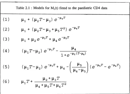
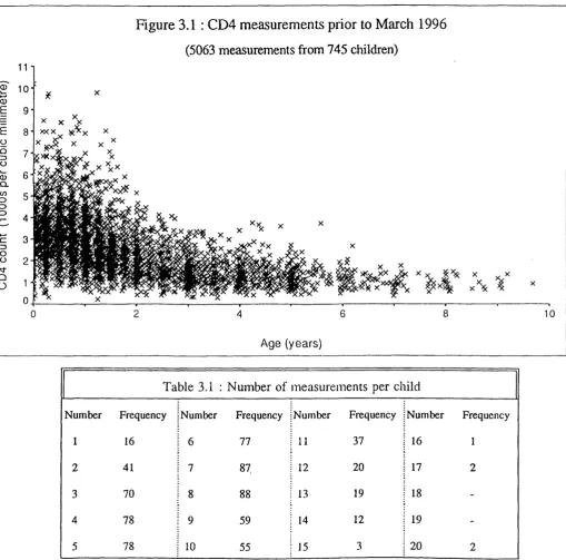
3.1 Introduction... 66 3.1.1 The dataset
3.2 M eth o d s... 70 3.2.1 Developm ent o f likelihood
3.2.2 Estimating the correlation structure
3.2.3 Estimation o f correlation and reference standard parameters
3.3 R e s u lts... 75 3.3.1 Gentile precision
C H A PT E R 4 : O R D IN A L O U T C O M E S
4.1 Assessm ent o f visual acuity in ch ild ren ... 90 4.1.1 The datasets
4.2 M e t h o d s ... 94 4.2.1 Goodness-of-fit
4.2.2 Achieving specified failure rates at chosen ages 4.2.3 Confidence intervals
4.2.3.1 Sample size estimation
4.3 R e s u l t s ... 98 4.3.1 Goodness-of-fit
4.3.2 Achieving specified failure rates at chosen ages 4.3.3 Confidence intervals
4.3.3.1 Sample size estimation
C H A P T E R 5 : C O N C L U S IO N 113
R E F E R E N C E S 120
A P P E N D IX 1 : C O M P U T A T IO N 138
A P P E N D IX 2 : P U B L IC A T IO N S 141
T a b le s
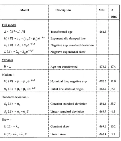
1.1 Requirements for age-related reference range construction methods . . . . 17 2.1 M odels for M /t) fitted to the paediatric CD4 d a ta ... 56 2.2 Exponentially damped line and variants : M aximised log-likelihoods
(MLL) and tw ice the absolute difference between reduced m odels and the full
m o d e l... 59 2.3 Comparison o f reference ranges obtained from paediatric and adult data . . 63 3.1 Number o f measurements per c h ild ... 69 3.2 Distribution o f 18560 within child measurement pairs according to the 76 nearest protocol specified a g e s ...
3.3 Maximised log-likelihoods for a variety o f correlation structures and 81 m odels for the m e d ia n ...
3.4 Confidence intervals for the 5th centile and internal width o f the inteiwals 84 expressed as CD4 counts and as z - s c o r e s ...
4.1 Visual acuity by age group in 1140 ch ild ren ... 92 4.2 Maximum likelihoods obtained for a variety o f fractional polynomial
models fitted to the CD4 d a ta ... 100 4.3 Functions o f parameters o f practical interest : estimates and 95%
confidence in terv a ls... 107 4.4 Profile likelihood 95% confidence intervals for the pass rates using
Figures
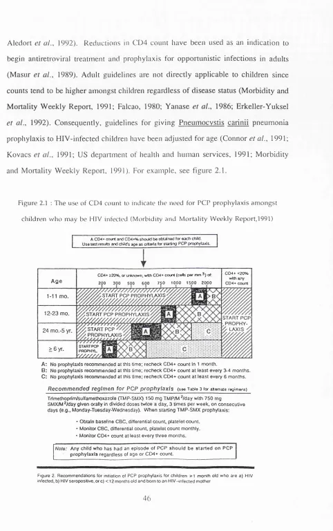
2.1 The use o f CD4 count to indicate the need for PCP prophylaxis amongst children who may be HIV infected (Morbidity and Mortality W eekly Report,
1 9 9 1 ) ... 46
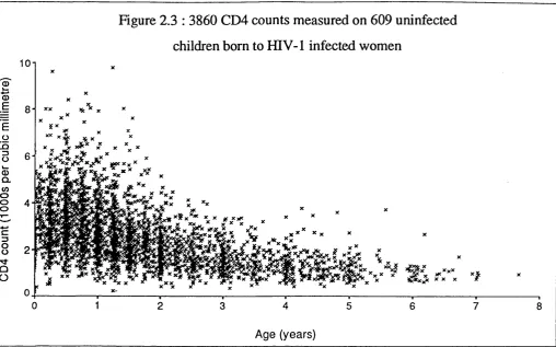
2.2 Current standards from birth or infancy for the CD4 counts o f uninfected children at risk o f HIV in f e c t i o n ... 48-49 2.3 3860 CD4 counts measured on 609 uninfected children born to HIV-1 infected w o m e n ... 51
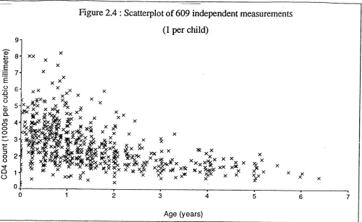
2.4 Scatterplot o f 609 independent measurements (1 per c h i l d ) ... 52
2.5 Selected fitted c e n t i l e s ... 61
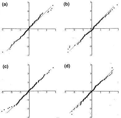
2.6 Normal probability plots for consecutive groups o f 152 measurements . . 61
2.7 Selected centiles and 95% confidence in tervals... 62
3.1 CD4 measurements prior to March 1996 ... 68
3.2 Empirical 5th, 50th and 95th centiles within blocks o f 101 consecutive m ea su r em en ts... 69
3.3 Maximum likelihood estimates within blocks o f 101 consecutive m e a su r em en ts... 69
3.4 Unsmoothed correlation estim a tes... 77
3.5 Distance dependent correlation structures... 78
3.6 A ge and distance dependent correlation structure (a) by age at first measurement (b) by time distance between m easurem ents... 79
3.7 Fitted centiles assuming independence and age and time dependent correlations... 83
4.1 Visual acuities o f 1140 ch ild r en ... 93
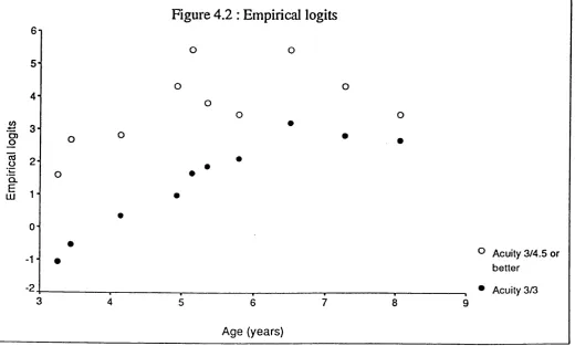
4.2 Empirical lo g i t s ... 98
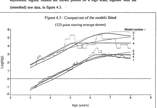
4.3 Comparison of the models f it t e d ... 102
4.4 The asymmetric logistic model on a probability s c a le ... 103
4.5 Letter sizes giving 85,90 and 95% pass-rates assuming the model parameters are linear functions o f letter s i z e ... 105
4.6 Distances (metres) from letters o f sizes 3/3 and 3/4.5 giving 90 and 95% p ass-rates...■ ... 105
4.7 Letter sizes giving 85,88,90,92 and 95% refenal across the age range . . 109
4.8 Confidence limits obtained at ages 4,4.75 and 6.5 years using data samples o f sizes 1140,2280,4560,6840 and 9 1 2 0 ... 109
CHAPTER 1
INTRODUCTION
1.1 : AGE-RELATED STANDARDS: AN OUTLINE OF THE PROBLEM
Clinical measurements from individual patients may be placed in the context o f population values using centile reference charts. These centile charts, som etim es known as reference ranges or normal standards, give the range o f values that the majority of a particular population are expected to lie within. Individuals with measurements outside the range may be investigated further. The effects o f covariates on the reference range may need to be taken account of. In paediatric medicine in particular, age-related reference charts, such as the height and weight standards, are being constructed for an increasing number of biological measures. D iscussion w ill be about age-related standards for simplicity. The methodology is similar for standards which change according to any continuous covariate and has many wide-ranging applications including those outside of medicine (for example: Bushby et al., 1992; Campbell & Robinson, 1993; Mahaney et al., 1993a; Mahaney et al., 1993b).
The methodology for the construction of age-related standards has been a subject for discussion for more than 40 years (Tanner, 1952). It has long been recognised that centiles estimated by combining the mean and standard deviation at each age are more precise than raw centiles (Tanner, 1952; Healy, 1974) and that standards should change smoothly with age to be biologically feasible (Tanner et al., 1966; Isaacs et al., 1983). Yet even today, implausibly erratic centiles calculated from the raw data are commonplace (for example: Wiedemann et al., 1993; Morgan e t al., 1996). Ideally, there should be a formal statistical basis for choosing the appropriate models and for assessing the fit o f the final model. Diagnostics should be available that identify any areas o f poor fit. For some applications, it may be adequate to state that an individual lies below the xth centile, where x is usually the 3rd or the 5th. However, exact standard deviation scores are more precise and may be especially useful for research purposes (Cole, 1990; Preece, 1989). Having a m ethodology that
allows for easy computation of the scores would therefore be advantageous. Centiles for the same parameter constructed using different datasets do not always agree (Lumley et al., 1971; Wright et al., 1993; Karlberg et al., 1985; Nwosu et al., 1993; White et al., 1995). Confidence intervals for the centiles would show to what extent apparent inconsistencies between standards for the same parameter may be due to inadequate sample sizes. Furthermore, confidence intervals for any standard deviation scores obtained from the models would aid interpretation.
A problem specific to paediatrics is that childhood measurements are often expected to asymptote at adult values. These adult values, and the age at which they are attained, may be known or unknown. For som e measurements children mature at different rates to all achieve the same final adult level. For example bone age will eventually reach maturity and in this case all the centiles would be expected to asymptote at the same level. Any information about the form or asymptotic values o f the parameter for which standards are being developed should be incorporated into the modelling procedure.
The standards must be constructed using a representative dataset for them to be clinically useful. Ideally the sample should be randomly collected from the population to which the standards will ultimately be applied (Yudkin et al., 1987). Where an individuals’ measurement will vary according to their prior characteristics, these characteristics may be included in the m odelling process. For example, predominantly breast-fed babies tend to be lighter throughout the first year o f life (Sheard, 1993), weight-for-height standards should take account o f pubertal physiological development (N g ’Andu et al., 1992), bone mineral content is dependent on both weight and height (Bishop et al., 1992) etc. (Tanner et al., 1970; Gardosi et al., 1992). Standards which do not take account o f differences between the groups of individuals will be both biased, for example a greater proportion o f breast-fed babies will appear to be
underweight, and imprecise, since the variance o f the pooled groups will be greater than for any single group (Preece, 1989). W e would expect smooth relationships between the centiles for the subgroups. For example, in the simplest case all the centiles may differ by a constant from one subgroup to another. Methods which jointly estimate the centiles w ill make more efficient use of the data than those which estimate them separately for each subgroup (Healy, 1974). However, there may be individual characteristics, for example social class, for which adjustment may be clinically inappropriate.
Where more than one measurement is taken from each individual then the approach has been either to take account o f the correlations between the repeat measurements (Royston and Altman, 1995), or to include only uncorrelated measures in the construction process (Thompson & Theron, 1990; Royston, 1991a; Altman and Chitty, 1994; Zorzoli et al., 1994). The latter alternative is the least efficient solution since it is wasteful o f the available information.
This introduction w ill firstly review the published methodology for the construction o f age-related standards. Only cross-sectional standards, which describe how an individual ranks in comparison to others o f the same age irrespective of previous values, are considered. It should be stressed that these are not necessarily suitable for the monitoring o f an individual over time since individuals may not always be expected to track centiles. For example, during adolescence children have growth spurts at different ages and the mean curve may not characterise the growth pattern o f an individual child. Velocity, or longitudinal, standards may be used to monitor changes over time (Moore et a i , 1954; Tanner et a i , 1966) Their construction w ill not be discussed. Neither w ill conditional standards (Royston, 1995) which are adjusted to take account of an individual’s previous values, be considered in this review.
Table 1.1 lists both the specific and more general requirements desirable for the ideal set of standards. The published methodologies will be discussed in turn with reference to their abilities to meet these requirements. In the concluding section the present state of the art is summarised and areas where existing methods could be advanced are outlined.
T able 1.1 : R eq u irem en ts for age-related referen ce ran ge con stru ctio n m e th o d s
S p ecific to reference ran ges
(1) T he p aram eters w h ic h d escrib e the d istrib u tio n (for ex a m p le, the m e a n and sta n d a rd d e v ia tio n ), an d h en ce the cen tiles, s h o u ld ch a n g e c o n siste n tly w ith age.
(2) There s h o u ld b e a form al statistical b a sis for c h o o sin g the a p p ro p ria te m o d els.
(3) G o o d n e ss-o f-fit sh o u ld b e a ssessed form ally. (4) D ia g n o stic s are n e e d e d to a ssess w h e r e fit is bad.
(5) T here sh o u ld b e a sim p le algorithm for ca lcu la tin g stan d ard d e v ia tio n scores.
(6) T here sh o u ld be a practical m eth o d for ca lcu la tin g co n fid en ce in terv a ls b oth for the cen tiles a n d for a n y sd -sco res su b se q u e n tly o b ta in ed u s in g them . (7) W h ere em p irical e v id e n c e su g g e sts that cen tiles a sy m p to te at a d u lt le v e ls,
the fo rm o f the eq u a tio n s sh o u ld reflect this.
(8) It sh o u ld be p o s sib le to incorporate a d d itio n a l covariates (categoric or n u m eric) w h e r e th ese sig n ifica n tly im p ro v e the fit o f the centiles.
(9) W h ere there are m u ltip le m ea su rem en ts p er in d iv id u a l, th ese sh o u ld all be in c lu d e d in the m o d e llin g p ro ced u re w h ic h s h o u ld in corporate an y correlation structure that is present.
G eneral to cu rve fittin g
(1) M a n y m o d e ls are su scep tib le to 'e d g e effects'. It w o u ld b e d esirab le to a v o id th ese, e sp e c ia lly in p aed iatrics w h e r e it is o ften essen tia l to h a v e accurate sta n d a rd s from birth.
(2) O u tliers m a y u n d u ly in flu en ce an y m o d e l and their effect sh o u ld b e m in im ise d .
(3) G r o u p in g o f the data prior to m o d e l fittin g is u n d e sira b le sin ce it m a y lea d to o v er sm o o th in g .
(4) O v e r-fittin g s h o u ld a lso be a v o id ed .
1.2 : METHODOLOGY FOR CONSTRUCTING STANDARDS
1.2.1 Early developments and ad hoc approaches
Early attempts to produce centiles that changed smoothly with age consisted o f finding the ’best fitting curves’ through the centiles calculated from the mean and standard deviation in several adjacent age groups either simply "by eye" or "using a flexible lead spline as a guide" (Tanner et a i , 1966). It was recognised that dividing the data into age groups could lead to the standard deviation being over-estimated if the mean changed with age. The standard deviation used in these early attempts was therefore adjusted according to the extent of age-related changes in the mean within each age group (Healy, 1962; Goldstein, 1972; Cleveland et al., 1989). The reason for not using mathematical methods of fitting was that cuiwes of the appropriate fonn "could not be fitted efficiently and expeditiously by a computer program at the time o f writing" (Tanner et at., 1966). A major advantage of fitting graphically rather than by computer was noted to be that the researchers "were not constrained by having to fit a preselected curve o f known form" and, if thought reasonable, they "could let a dip in the curve remain, rather than smooth it out". The fact that "a certain amount of sleight-of-hand" was involved in the consuuction o f standai'ds was openly acknowledged by som e authors (Tanner, 1958). Sometimes smooth fitting centiles were presented without any explanation of how they were obtained from the raw data (Thomson et at., 1968). Later applications used polynomial regression to join centiles estimated from adjacent blocks of data points (Yudkin et at., 1987).
For skew data it was necessary to first transform the data. If skewness changed with age, then one single transformation to normalise the data would not be adequate. Karlberg et at., 1985, used the most appropriate B ox-C ox transformations of
birthweight at each week of gestational age (Box & Cox, 1964). After calculating the mean and upper and lower probability limits of the normalised data, these were back-transformed and cubic splines used to smooth the estimates from the different weeks.
D ibley et al., 1987, avoided the need to decide on a suitable transformation and coped with age-related changes in skew by considering the data above and below the median separately within each age band. A standard deviation for those below the median was calculated from the raw 5th, 10th, 25th and 50th centiles, this standard deviation was then used in the calculation o f centiles below the 50th. A similar process was used for centiles above the 50th. The resulting centiles were smoothed by polynomial regression and cubic splining techniques.
1.2.2 The LMS Method
Isaacs et al., 1983, modelled the mean and variance before combining them to create centiles. Log and square root transformations were used to normalise the IgG, IgA and IgM values obtained from children between 6 and 72 months o f age. A polynomial was fit to the transformed data and the residuals divided into groups. Tlie standard deviation of the residuals in each group was calculated and another polynomial fitted to these to describe age-related changes in the standard deviation. The polynomials for age and standard deviation were combined and back-transformed to create centiles that changed smoothly and consistently with age. Royston, 1991a, used a similar approach with a modified logarithmic transformation o f the form logg(y+C).
V an’T H of et al., 1985 coped with changing skewness across the age range by creating a third curve, L(t), that described those changes in skewness. This curve was chosen to summarise how the best-fitting Box-Cox transformations to
normality, X g , changed across age groups
^9
l o g / j g ( ^5 =0 )
where y^g is the ith observation in group g; g = i = l,2,...,Ug is the number o f observations in group g; ni+U2+...+ng= N.
Each data point was transformed using the Box-Cox transformation indicated by the fitted curve, L(t). The mean and standaid deviations o f the tiansformed data in each age group were calculated and "eye-fitted smooth cuiwes drawn" (Mi(t) and Si(t) respectively) to give values across the age range. Centiles for the transformed data were calculated from the smoothed mean and standaid deviation and subsequently back-transformed using the smoothed skewness parameters. They noted tliat a standard deviation score could be calculated for an individual at any age in the range using the
formula:-for values L { t ) ^ 0 , where Y is the individual’s actual value and Mi(t) and S / t ) are the mean and standard deviation of the transformed data at the appropriate age. A similar equation could be derived for the case where L(t)=0.
Cole, 1988, m odelled tlie coefficient o f variation rather than the standaid deviation since this was more likely to be independent o f the mean for many medical applications. The other contribution he made was to use mathematical models to fit curves to the median, the Box-Cox parameter that induced normality and the coefficient of variation. He called the resulting cui*ves the M, L and S cuiwes
respectively and noted that the curves describing the median (M^Ct)), coefficient o f variation (S2(t)) and the skew (L(t)) may be of interest in their own right (Cole, 1989).
The equation of the 1 0 0 a t h centile at age t was given by
(1.2)
( L( t ) = 0 ) ( 1 . 2 a )
where is the normal equivalent deviate for tail area a . The standard deviation score, z, for an individual with a measurement o f Y at age t could easily be calculated using the equation
z = M A t )
L i t ) - 1
{ L i t ) * 0 ) ( 1 . 3 )
l o g z =
^ y '
M , { t )
S , ( t ) ( L i t ) = 0) ( 1 . 3 a )
He recognised that to use this method the data must be normally distributed on an appropriate power scale. To limit the detrimental effects o f blocking the data, he suggested choosing groups sufficiently narrow for the trends in the median, skew and coefficient o f variation across them to be essentially linear.
1.2.3 A Maximum Likelihood Approach
Thompson & Theron, 1990, assumed that a Johnson density was an appropriate model for each o f several age groups and that the parameters o f these densities changed
smoothly over time. For example, using the Johnson Sy distribution
= E + ^ , s i n h
/ A
y j g - l
Tic g
y
( 1 . 4 )
where is the measurement for the i th subject in age group g; is distributed standard normal and the log-likelihood expressed as
( 7 , + %i o g [ "
+ logilg-logl^-_^ log (1+wf^) ] (1.5)
where ; g = l , 2 , . . . , G age groups; i = 1 , 2 , . . . . , is the
g
number o f individuals in age group g. X^, and are expressed as suitable functions across age groups. For example, if e is approximately quadratic, then this could be entered into equation (1.5) as + j b ^ g + a n d parameters , jb^, chosen to maximise the log likelihood.
The equation of the 1 0 O a t h centile for age group i could be calculated using the formula
Citio.(g) =êj, + îjS in h
( 1 . 6 )V
The asymptotic variance of the centile for that age group could also be evaluated using a Taylor series approximation.
Thompson & Theron, 1990, used the described method to create standards charting weight gain during pregnancy. There was good agreement between the asymptotic variances o f the centiles using the maximum likelihood approach and jackknife estimates o f the variances.
1.2.4 Non-parametric Methods
Healy et al., 1988, introduced a non-parametric approach avoiding the need to make any distributional assumptions at any given age. They used scatterplot smoothing (Cleveland, 1979) to produce selected centiles from the raw data. It was assumed that the curve for each o f the centiles could be fitted by a polynomial o f degree p
Cioo«(t) =ao«-^ai,t + a2„t2+ . . . +a^c;'
( 1 . 7 )
where t denotes age and C^ooo ( the smoothed value o f the l OOcc th centile at age t. They constrained the model parameters to vary consistently between centiles by adding the restriction that
where is the normal equivalent deviate for tail area OC . The degree Qj of the polynomial was allowed to differ from one value of j to another. Combining (1.7) and (1.8) gave a linear model for the chosen set of centiles that could be fitted using least squares.
Pan et a i , 1990, replaced equation (1.7) by
Ciooa(fc) = a o . + a i . ( : + . . . . . .
P
+ ( 1 . 9 )
where
( t - C j ) += ( w h e n t > C j
= 0 w h e n i = l , 2 , . . . , m- 1
Cj is the 1 t h cut or join point between the age groups with
< Cj < . . . < c^ _ i. The values of m and c, were "chosen after inspection o f the data and using existing knowledge". "The choice of the number and placing of join points in this method" was "a matter for experimentation".
These modified curves, sometimes known as piecewise or grafted polynom ials, have continuous derivatives and allowed greater flexibility in the shapes that could be fitted using relatively low order polynomials (Pan et a i , 1992). Goldstein & Pan, 1992, noted that the approach is preferable to a more general cubic spline with which joint smoothing would be very complicated.
The method entailed an arbitrary choice of centiles to include in the modelling process. A flexible approach suggested by Goldstein & Pan, 1992, was to weight each chosen percentile so that the effect o f varying these weights could be explored. In this case, a matrix o f weights would be incorporated into the model and the generalised least squares solution obtained in the usual way. In the most general case, consider a set o f weights, w^, for the jth data point and ith percentile, with no restriction on the structure o f W={W|j}. However, in many applications, it would be sufficient to write Wjj in the form WjWj where the Wj specify common weights for the ith percentile and the Wj specify common weights for the jth age. They noted that the usual caution is necessary when making extrapolations to percentiles beyond those estimated from the raw data.
Rossiter (1991) simulated datasets from known distributions and applied kernel density estimation (Hastie & Tibshirani, 1990) using bandwidths that changed throughout the covariate range to create centiles. With a uniform kernel over a finite range and constant bandwidth this method would therefore be the same as H ealy’s moving average. The sum o f the squared errors between the true and estimated centiles was used as a measure o f the appropriateness of each model. This method indicated the
optimal bandwidth s to use throughout the range and illusU ated that departures from the optimal bandwidths had a greater effect on the model fit at the extremes o f the data. Using a large bandwidth at the tails o f the distribution helped to overcome the problem o f edge effects, whereas a smaller bandwidth at points in the main body of the distribution ensured that modes were not underestimated. By converting data collected on the kidney lengths and birthweights o f newborn infants to a form similar to the original simulated data, the previously determined optimal bandwidths were used to create smoothly changing standards relating kidney length to birthweight.
1.2.5 Block-free Methods
A ll o f the above methods, as they were originally presented, rely on some form o f arbitrary grouping, or ’blocking’, of the data. The choice o f block size may influence the final results. In particular, blocking leads to over-smoothing where the 2nd derivative is appreciable. However, many o f the presented methods either have been or can be extended.
Blocking is easily avoided if the data, or some transformation, has constant standard deviation across the age range. For example, Davies et a i , 1992, used log transformation prior to fitting cubic polynomials to model the changes in several blood parameters with gestational age. The residual standard deviation was used to create centiles on the tiansformed scale, which were then antilogged. Snijders & Nicolaides, 1994, used a similar approach with square root and shifted log transformations. Bland
et al., 1990, used a log transformation to remove heteroscedascity before regressing
birthweight on gestational age and a further transfonriation to nonrialise the residuals from the fitted model. The centiles of the normalised residuals were then combined with the model for the median to give centiles for birthweight according to gestational age.
Altman, 1993, suggested using a transformation that is a function of age, for exam ple log(Y +c(age)), before modelling the mean and regressing the absolute residuals on age. Since the mean of a half standard normal distribution is ^ 2 , the mean o f the absolute residuals multiplied by gives an estimate o f the standard deviation of the residuals. If the standard deviation changes with age then the predicted value of a regression o f the absolute residuals on age multiplied by w ill give estimates o f standard deviation across the age range. Hence, each observation contributes to the age specific estimates of the standard deviation. He suggested that these estimates could be used inversely as weights for the observations and the mean curve re-estimated using the weighted observations in the manner suggested by Aitkin, 1987. The advantages o f this method were that it avoided any grouping of the data and coped with non-linear changes in variance with age. However he noted that the skewed nature of the residuals invalidated the usual hypothesis testing o f the model parameters. Standard deviation scores could readily be calculated for any observation. The method was used to calculate standards for fetal measurements by gestational age (Altman & Chitty, 1994; Chitty et al., 1994).
Cole & Green, 1992, were the first to model skew in conjunction with the median and standard deviation while avoiding blocking by combining maximum penalized likelihood (Silverman, 1990) with the LMS method. Using this approach, the L(t), M2(t) and S^(t) curves were estimated by maximising the penalized likelihood:
{ t ) ] ' ‘‘d t - ^ a ^ j [ S - ! , ' { t ) ] ' ^ d t ( 1 . 1 0 )
where:
L ( t ) l o g V
- l o g S ; i t ) 1.11)
is the log likelihood o f the observed z (or standard deviation) scores of N independent
observations, y,, and the a values are smoothing parameters. Using the squared second derivatives as roughness penalties gives natural cubic splines with knots at each distinct value o f This method removed the need for age blocking o f the data, the only arbitrariness being in the choice o f smoothing parameters.
Thompson & Theron, 1990, used maximum likelihood to "simultaneously fit a density at each cross-section" (equation (1.5)). However, blocking could easily be dispensed with by considering each observation to be a separate ’block’ o f data. That is, replacing equation (1.5) with
1/= 52^. [ - - ^ ( Yi+Tli l o g [ ] ) ^+ l o g r \ ^ - l o g X . - ^ l o g [ l + w]) ] ( 1 . 1 2 )
' —£
where there are i= l,2,...,N observations; w^ = —L__ i and e ^ , X - , y ^ and r|_j. are
k.
suitable functions o f age (e.g. e. = a^ + b^t^ + c ^ t j , t; being the age at which obsei*vation y-^ was made).
Similar adjustment could be made to calculate centiles from equation (1.6) although calculation o f the variances would not be straightforward.
1.2.5.1 Asymmetric Least Squares
Koenker and Bassett, 1978, proposed the use of asymmetric absolute loss to define regression quantités and to give a more robust estimate o f the median than ordinary least squares estimation. Efron, 1991, noted that a similar technique, asymmetric least squares regression, could be applied specifically to determine regression percentiles for their own sake and to calculate a range of centiles. The method, simply a variant o f ordinary least squares with different weighting given to positive and negative residuals, consisted o f finding the best fitting polynomial independently for each centile. The range o f centiles was produced by progressively changing the balance of
the residual weightings. Thus, centiles were not constrained to behave consistently in relation to each other. Hence commonality between adjacent centile curves is not a pre-requisite o f the method. Furthermore, it would not be known which particular centile was being fitted with a given weighting. This needed to be determined after completion o f the fitting process by counting the points above and below the resultant centile line.
1.2.5.2 Multilevel Modelling
Where serial measurements are made on each individual, one possibility is to fit a regression curve to each individual’s data. These curves should be o f the same shape but with different parameters for each individual. The variation o f the parameters between individuals can be used to enable the creation of cross-sectional standards (Tanner et a i , 1966). For example, Gallivan et al., 1993 modelled ultrasonic measurements for each o f 67 fetuses who were followed longitudinally. They interpolated the resulting curves to give measurements at exact gestational ages between 20 and 40 weeks. These interpolated values were then used to create gestation-related standards which could be used cross-sectionally. However, because the within subject variability has been ignored, this approach w ill lead to centiles that are too close together (Altman & Chitty, 1994; Royston, 1995; Nash et al., 1996).
M ultilevel modelling (Goldstein, 1986) was introduced as a means o f investigating the variability o f hierarchically structured datasets. Using this method, the modelling of the individual curves is not separated from the construction o f the cross-sectional standards and so the within child vaiiability is retained in the final model (Busch an g
et al., 1989). In the simplest and most usual case, the measurements constitute the
le v e l-1 units and children the level-2. The method is however also appropriate for some situations where there are single observations per individual. For example. Pan
et a i , 1992, used multilevel modelling to construct age-related centiles for children from several distinct districts; each child’s measurement was a le v el-1 unit and districts were level-2 units. The method is flexible and readily incorporates data transformations where this is necessary to establish a form amenable to the fitting of individual curves. For example, Royston, 1995, used a Box-C ox transformation o f the outcome variable to reduce non-normality and heteroscedasticity of the residuals as w ell as maximising the parallelism o f the response curves. The covariate values were then transformed using a fractional polynomial (Royston & Altman, 1994) before modelling the responses for each subject as a straight line function
:-= ( 1 . 1 3 )
Iny^-
(X,=0)where i=l,2,...,nj is the number of observations from the j th individual and
9 ^^i j ) is a continuous function o f the observation times. The parameters
[ij and pj (the regression intercept and slope for the j th subject) were introduced into the model as random variables having a bivariate nonnal distribution. The within-subject residuals were assumed to be independent and normally distributed with zero mean and a variance Og for all subjects. Equation (1.13) is a two-level model wi t h p a r a m e te r s Og and the m e a n s , v a r i a n c e s and c o v a r i a n c e of and p j . Parameter estimates were obtained using maximum likelihood to compare nested models formally by considering the difference in the model deviances. To test the significance of the Y transformation, the likelihood was divided by the Jacobian o f the transformation o f the y^ prior to calculating the deviance (Atkinson, 1987). The mean and variance o f the transformed measurement Z = Y ^ at transformed time X=g(T) were calculated:
Z(Z) =|ig = p + P%
( 1 . 1 4 )
V( Z) = a l = a l + x ^ o l + 2 X a ^ p + a i ( 1 . 1 5 )
Cross sectional centiles at any time point could be calculated from (1.14) and (1.15).
Goldstein et al. , 1994, showed that autocorrelations between the le v el-1 measurements could be incorporated into the models by removing the assumption that the e . j are independent. The e.^. could be modelled either as an autoregressive (AR) process or as som e function o f continuous time. The latter approach has the advantage that the data are not assumed to be at discrete equally spaced time intervals.
1.3 AN ASSESSMENT OF THE APPROACHES
Various methodologies for the construction of smoothly changing age-related standards for a continuous parameter have emerged over the years. The asymmetric least squaies and multilevel modelling approaches were somewhat novel, but it is unclear that these could cope with changes in skewness across the age range without prior transformation. Three methods, namely non-parametric, LMS and maximum likelihood, possessed the ability to deal with most potential age-related changes in the median, spread and skew. The dependence of the non-parametric approach on initial centile smoothing meant that an arbitrary choice o f grouping o f the data could not be avoided. A further consequence of this necessity to group was that the resulting standards extended only from the mid-point of the first group of data to the mid point o f the last. In paediatric medicine this may pose a particular problem since standards are often required from birth. Rusconi et al., 1994, countered this problem by oversampling near to birth and including infants older than 3 years of age when constructing reference ranges for the respiratory rates o f children in the first 3 years of life. The main advantage o f the non-parametric approach is it’s ability to allow for anv com plexity o f distributional changes with age. Arbitrary age grouping was not an inherent part o f the other two methods. This was illustrated by Cole & Green, 1992, and equation (1.12).
1.3.1 Curve forms
All o f the methods involved some modelling and the choice of model forms used by individual authors has varied. There is no reason however why any of the methods could not be modified to incorporate any o f the suggested forms. Simple polynomials have often been used (Isaacs et a i , 1983; Healy et a i , 1988; Thompson & Theron, 1990; Bland et al., 1990; Efron, 1991; Davies e t a i , 1992; Chitty et al., 1994) but these are limited in the shapes that can be modelled without inclusion o f high order terms. Exponential models, for example the Gompertz and Rossavik models (Gallivan
et al., 1993), are also restricted in the variety o f shapes that can be modelled within
a uniform framework. The family o f Laguerre polynomials (Jones, 1996) gives a wide variety o f models all of which asymptote. Cubic splines (Karlberg et al., 1985; Dibley
et al., 1987; Cole & Green, 1992,Cole et al., 1995) allow greater flexibility but may
be unnecessarily complex (Goldstein & Pan, 1992). Piecewise or grafted polynomials (see equation (1.9)) have been suggested as an alternative (Pan et al., 1990; Pan et al.,
1992; Goldstein & Pan, 1992). Fractional polynomials, o f which conventional polynom ials are a subset, may be preferable since join points do not need to be established and iterative algorithms for model selection are available. Royston & Altman, 1994, demonstrated that the algorithms yielded more appropriate models for the median values of the IgG and fetal measurements previously described using conventional polynomials (Isaacs et al., 1983; Altman, 1993).
1.3.1.2 Edge effects
Som e model forms are more susceptible to edge effects and tliese should preferably be avoided. Fractional polynomials appear to offer more stability at the data extremes although they may behave inappropriately near to zero (Royston & Altman, 1994). Cole & Green, 1992, suggested that edge effects could be minimised by increasing the
density o f observations at the extremes of the age range and that increased density may also be advantageous at other ages where there is rapid change.
1.3.2 Outliers
Outliers may unduly influence any model. The extent to which they cause a problem w ill depend both on the form of the model used and the method o f centile estimation. Cole, 1988, questioned the extent to which outliers would affect the estimates o f skew in his formulation. He suggested trimming the data (by deleting the largest and smallest values) and examining the change in the obtained lambda value, omitting these extreme values if there was appreciable change, then repeating the process until stability was achieved. However, he noted that the estimates of the variance after trimming would be biased downwards progressively and suggested possible adjustment by fitting a doubly truncated normal distribution (Healy, 1978). The variance would be similarly biased by a method used by Palmer et a i , 1992. They grouped the data into monthly intervals and excluded all observations more than 2.5 standard deviations from the mean before proceeding with the fitting process. Karlberg et a i , 1985 used the more arbitrary approach o f truncating birthweights at different gestational ages to a "range where the observations seemed entirely plausible" prior to calculating centiles for birthweight by gestational age. Their argument that this truncation would not introduce bias but "at worst bring a little inefficiency" is clearly dubious.
Independence is introduced into the fitting o f individual centiles with the non-parametric and asymmetric least squares approaches and hence outliers have potentially more influence. Healy et a i , 1988, noted the vulnerability of their non-parametric approach to outliers, although their effect on the initially smoothed centiles would be diminished by the application of equations (1.7) and (1.8). Their suggested
solution was to use a robust regression approach (Cleveland, 1979) to identify and eliminate outliers prior to model fitting. Efron, 1991 suggested calculating the maximum percentage influence of each data point on centiles determined using asymmetric least squares and removing data values with a high influence. The centiles obtained from the complete data set could then be compared to those calculated from the reduced data set and a decision to exclude or include the outlying point(s) made on the basis o f this comparison.
1.3.3 Choice of model
Ideally there should be a formal statistical basis for choosing the appropriate models within the selected form. Although not explicitly stated by Thompson & Theron, 1990, the usual significance tests comparing nested models could be used to determine the degree o f the polynomials used to represent time related changes in the model parameters e^, X . , , y . . The non-parametric approach (Healy et al., 1988) was limited by the fact that successive points on a single centile are highly correlated and there are also correlations between simultaneous points on adjacent centiles. Although the fitted curves would not be biased by these correlations, they do invalidate the conventional calculation of standard errors o f the coefficients.
1.3.4 Goodness-of-fit and diagnostics
Quantifying how well the centiles fit has previously been described as something of a "black art" (Cole, 1988). The difficult being in deciding " whether a bump or dip observed on a centile curve at a particular age is a real feature o f the data, of whether it is simply sampling error" (Cole & Green, 1992). The LMS method simplified the
problem somewhat since decisions need only be made regarding 3 uncorrelated curves, the L, M and S, rather than for 7 or more related centiles. An informal validity check suggested by Royston, 1991b, to assess the extent to which the fitted centiles adequately described the data was to verify that values falling outside the extreme centiles did not tend to cluster. Similarly, visual examination o f the empirical and model-based centiles was undertaken to establish that they agreed "fairly well" (Royston, 1995). More formal methods are complicated by the fact that adequate fit is required throughout the age range. For example, Rossiter, 1991, compared the number of points lying between pairs of successive centile curves with those expected using chi-square. However, this method may over-estimate the goodness-of-fit since poor fitting areas could cancel each other out. Similarly, whilst standard methods, for example, the Shapiro-Wilk W test, examination of a normal plot etc., can be used to assess the normality of the z-scores o f the fitted centiles (Bushby et al., 1992; Altman & Chitty, 1994), an adequate fit overall does not imply good fit throughout. Consequently, some grouping o f the age range prior to investigation is necessary. For example, Van’T H of et al., 1985 calculated the empirical percentages contained between the centiles for each half of the age range. Healy et a i , 1988, Cole, 1988 and Wright & Royston, 1997 used the same approach with an increased number of age groups. Wright & Royston, 1997, present the chi-square statistics obtained both with and without any age grouping and these clearly highlight the inadequacies of the latter. They address the arbitrary nature of these goodness-of-fit tests, noting that "the assessment o f goodness-of-fit is an area requiring further research ... Questions of the power o f different procedures and the sensitivity to the number o f age gioups and/or centile curves chosen should be addressed."
Dibley et al., 1987, considered normal plots for different age groups. Cole, 1988, also used Shapiro-Wilks’ W statistic to verify the normality o f the data within age blocks after B ox-C ox transformation. Goldstein & Pan, 1992, calculated the proportion falling
below the 3rd, 50th and 97th centiles within blocks of 100 consecutive points. These proportions were then plotted against the expected values and the resultant charts visually inspected to determine any areas of poor fit. A different approach was taken by Freeman et a i , 1995, who compared the number o f observations below the 3rd, 50th and 97th centiles in yearly intervals with the expected number to produce 3 statistics at each age. The distribution o f these individual statistics was then investigated. They give median and range by sex and note that these are "compatible with a standard on 1 df". Additionally "the spread o f the values showed no distinct patterns with age".
Assessment o f model fit is further complicated if serial measurements are used to construct the centiles. For example, model (1.13) used by Royston, 1995, implied that Z = y was normally distributed at any given timepoint. He checked this assumption by testing Z for non-normality at each timepoint but noted that the tests were not independent owing to the repeated-measures nature o f the data.
1.3.5 Standard deviation scores
A further disadvantage of the methods that independently evaluate the centiles is that standard deviation scores cannot necessarily easily be calculated from the final model(s). Using the non-parametric approach, standard deviation scores could theoretically be calculated for any given value at any age, the com plexity of the process though would depend on the orders o f the polynomials and the extent of grafting. Parametric forms that jointly estimate the centiles must, by definition, enable a formula to be given expressing any value in the age range as a standard deviation score. This property is illustrated in equations (1.3) and (1.3a) and a re-formulation o f equation (1.6).
1.3.6 Confidence intervals
Confidence intervals for the centiles can be derived using conventional methods as long as only a single standard deviation was estimated in the fitting process. This was illustrated by Chinn, 1992 who used a fitting algorithm similar to that o f Bland et a i ,
1990. Similarly, for non-constant standard deviation, confidence intervals could be evaluated within age groups. This was the approach taken by Cole, 1990. Since precision was greater than that implied by the sample size for the age group alone due to smoothing o f the L and S curves, he suggested "scaling up" the sample size to a "notional" value. He noted that the scaling factor would depend on "how the smoothing is done, and whether the particular age group is near to the centre or the extremes o f the age range studied". He concluded that "using a scaling factor o f 2 or 3 ought to be safe, if conservative". Thompson & Theron, 1990, calculated asymptotic variances for each block o f data and compared these to jackknife estimates, concluding that the former which are "a simple byproduct of the maximum likelihood estimation procedure" could be used as a reasonable guide to the precision o f the associated estimates.
Royston, 1995, noted that standard errors and confidence intervals for the estimated centiles could not readily be constructed using his methodology because o f the uncertainty of the parameter estimates used to transform the covariate. As an alternative, he systematically generated sets of data from the final model and re-estimated the centiles at various time points. The standard errors of each centile were smoothed across time points (using second degiee fractional polynomials) and confidence intervals constructed using the smoothed values. In the absence o f any formal derivation o f the standard error, bootstrap estimates (Efron & Gong, 1983; Efron & Tibshirani, 1986) can always be calculated (Altman, 1993).
1.3.6.1 Sample size
The sample size required to give curves precise enough to be clinically useful could be calculated by considering the width o f the confidence intervals for the centiles. Cole, 1990, discussed this issue and noted that having formulae for the standard errors o f the centiles enabled the derivation o f sample size formulae directly.
1.3.7 Asymptotes
When empirical evidence suggests that the centiles should asymptote at adult values, then the appropriate model can be chosen to reflect this. Exponential models and a subset o f the polynomials have the required property. Goldstein & Pan, 1992, suggested using the general inverse polynomial :
y "EL
(
1.
1 6)
for the final age range in a piecewise polynomial which could be constrained to pass through known adult values. Royston & Altman, 1994, noted that fractional polynomials with only negative powers asymptote. Hence, restricting the power set used by the fitting algorithm would yield the necessary model set. However, it is unclear how restrictive this may be regarding the rest of the curve. Healy et al., 1988, proposed fitting som e form o f non-linear curve to the initially smoothed median and then using the general method to fit simpler curves to the differences of the other centile points from this basic curve.
1.3.8 Additional covariates
The method o f fitting the centiles should have the ability to incorporate additional covariates where these significantly improve the fit. The necessity to incorporate a
covariate can be tested by fitting a model without any adjustment for covariates and examining the resultant z-scores in relation to the covariate values (Ayatollahi, 1995). Cole, 1988, suggested that the median curves could be fitted independently whilst using the combined data to estimate the curves representing the skew and the coefficient o f variation if these could reasonably be assumed not to differ between subgroups. The non-parametric (Goldstein & Pan, 1992) and multilevel (Pan et al.,
1992) m odels could easily be extended to incorporate different coefficients within subgroups. Goldstein & Pan, 1992, noted that the subgroups would usually only differ in terms o f the lower order polynomial coefficients. Efron, 1991, showed that the asymmetric least squares approach coped very w ell with two continuous covariates, a situation where visual inspection, and hence determination o f the relationship between the centiles for both covariates, is difficult. Royston & Altman, 1994, presented an algorithm for finding the best fitting fractional polynomial where there are several continuous covariates to be jointly fit. Cole, 1979, took account o f the dependence of weight for height on age by modelling weight for age as a function of height for age.
1.3.9 Serial measurements
Serial measurements from individuals may be already available. Alternatively, when collecting measurements for the sole purpose of constructing standards, it may be more feasible to repeatedly measure the same group over time. This latter scenario is particularly relevant in paediatrics where the available pool of children may be limited, either due to limited numbers currently with the condition (for example, children bom to HIV-1 infected women), or to the ethical and practical limitations involved.
multilevel modelling method for creating centiles. Autoconelations between measurements within individuals could readily be incoiporated with the autocorrelations themselves structured in terms of explanatory variables (Goldstein et
a i , 1994). However, although there are no restrictions on the number or timing of
observations per individual, the individual trajectories need to follow a specified format. A particular parametric form may be chosen or a more flexible approach, for example B-splines (Silverman, 1985; Shi et al., 1996), used.
Thompson & Theron, 1990, noted that their methodology could in principle be extended to explicitly include any correlation structure present in the data. Using the LMS and non-parametric approaches there aie no simple extensions to the methodologies to include correlations between serial measurements. However it has been suggested (Harrington et a i , 1995) that there is no need to make anv coiTection for the inclusion of multiple observations per individual using tlie non-parametric approach. This is due to the method’s dependence on the initial calculation o f centiles within subgroups o f the data. Since these subgroups span a limited range o f ages and hence rarely include more than one observation per individual, all centile calculations are based on independent sets o f measurements.
An alternative to extending the methodologies where deemed appropriate, is to use all available measurements and then test the residuals for non-independence. Draper & Smith, 1981, suggest graphical techniques as well as the more formal Durbin-Watson test. These techniques were used by Palmer et a i , 1992, who had included a mixture of cross-sectional and longitudinal data in their construction of centiles for head circumference. However, since the tests depend quite heavily on sample size and there are unlikely to be more than 5 or 10 measurements over time for each individual, the conclusions that can be drawn will be limited.