321 Abstract—Temperature warnings are important forecasts
because they are used to protect life and property. Temperature forecasting is the application of science and technology to predict the state of the temperature for a future time and a given location. Temperature forecasts are made by collecting quantitative data about the current state of the atmosphere. In this paper, a neural network-based algorithm for predicting the temperature is presented. The Neural Networks package supports different types of training or learning algorithms. One such algorithm is Back Propagation Neural Network (BPN) technique. The main advantage of the BPN neural network method is that it can fairly approximate a large class of functions. This method is more efficient than numerical differentiation. The simple meaning of this term is that our model has potential to capture the complex relationships between many factors that contribute to certain temperature. The proposed idea is tested using the real time dataset. The results are compared with practical working of meteorological department and these results confirm that our model have the potential for successful application to temperature forecasting. Real time processing of weather data indicate that the BPN based weather forecast have shown improvement not only over guidance forecasts from numerical models, but over official local weather service forecasts as well.
Index Terms—Multi layer perception, Temperature
forecasting, Back propagation, Artificial Neural Network
I. INTRODUCTION
Due to chaotic nature[8] of the atmosphere, the massive computational power is required to solve the equations that describe the atmosphere, error involved in measuring the initial conditions, and an incomplete understanding of atmospheric processes. This means that forecasts become less accurate as the difference in current time and the time for which the forecast is being made (the range of the forecast) increases. The use of ensembles and model helps narrow the error and pick the most likely outcome.
Several steps to predict the temperature are
Data collection(atmospheric pressure, temperature, wind speed and direction, humidity, precipitation), Data assimilation and analysis,
Numerical weather prediction, Model output post processing.
A neural network [1] is a powerful data modeling tool that is able to capture and represent complex input /output relationships. The motivation for the development of neural network technology stemmed from the desire to implement an artificial system that could perform intelligent tasks similar to those performed by the human brain. Neural
network resemble the human brain in the following two ways:
1) A neural network acquires knowledge through learning.
2) A neural network‟s knowledge is stored within interneuron connection strengths known as synaptic weights
The true power and advantages of neural networks lies in the ability to represent both linear and non linear relationships directly from the data being modeled. Traditional linear models are simply inadequate when it comes for true modeling data that contains non linear characteristics.
A neural network model is a structure that can be adjusted to produce a mapping from a given set of data to features of or relationships among the data. The model is adjusted, or trained, using a collection of data from a given source as input, typically referred to as the training set. After successful training, the neural network will be capable to perform classification, estimation, prediction, or simulation on new data from the same or similar sources.
An Artificial Neural Network (ANN) [5] is an information processing paradigm that is inspired by the way biological nervous systems, such as the brain, process information. The key element of this paradigm is the new structure of the information processing system. It is composed of a huge number of highly interconnected processing elements (neurons) working in unison to solve specific problems. ANNs, like people, learn by example. An ANN is configured for a particular application, such as pattern recognition or data classification, through a learning process. Learning in biological systems adds adjustments to the synaptic connections that exist between the neurons.
A back propagation network [9] consists of at least three layers (multi layer perception): an input layer, at least one intermediate hidden layer, and an output layer. In contrast to the Interactive Activation and Competition (IAC) neural networks (IAC) and Hopfield networks, connection weights in a back propagation network are one way. Typically, input units are connected in a feed-forward fashion with input units fully connected to units in the hidden layer and hidden units fully connected to units in the output layer. An input pattern is propagated forward to the output units all the way through the intervening input-to-hidden and hidden-to-output weights when a Back Propagation network is cycled.
As the algorithm's name gives a meaning, the errors (and therefore the learning) propagate backwards from the output nodes to the inner nodes. So technically it can be explained, back propagation is used to calculate the gradient of the
An Efficient Weather Forecasting System using
Artificial Neural Network
322 error of the network with respect to the network's modifiable weights. This gradient is always used in a simple stochastic gradient descent algorithm to find weights that minimize the error. Frequently the term "back propagation" is used in a more general sense, to refer to the entire procedure encompassing both the calculation of the gradient and its use in stochastic gradient descent. Back propagation regularly allows quick convergence on satisfactory local minima for error in the kind of networks to which it is suited.
The proposed Temperature Prediction System using BPN Neural Network is tested using the dataset from [17]. The results are compared with practical temperature prediction results [18, 19]. This system helps the meteorologist to predict the future weather easily and accurately.
The remainder section of this paper is organized as follows. Section 2 discusses various temperature predicting systems with various learning algorithms that were earlier proposed in literature. Section 3 explains the proposed work of developing An Efficient Temperature Prediction System using BPN Neural Network. Section 4 illustrates the results for experiments conducted on sample dataset in evaluating the performance of the proposed system. Section 5 concludes the paper with fewer discussions.
II. RELATED WORK
Many works were done related to the temperature prediction system and BPN network. They are summarized below.
Y.Radhika and M.Shashi [3] presents an application of Support Vector Machines (SVMs) for weather prediction. Time series data of daily maximum temperature at location is studied to predict the maximum temperature of the next day at that location based on the daily maximum temperatures for a span of previous n days referred to as order of the input. Performance of the system is observed for various spans of 2 to 10 days by using optimal values of the kernel
Mohsen Hayati et.al, [5] studied about Artificial Neural Network based on MLP was trained and tested using ten years (1996-2006) meteorological data. The results show that MLP network has the minimum forecasting error and can be considered as a good method to model the short-term temperature forecasting [STTF] systems. Brian A. Smith et.al,[6] focused on developing ANN models with reduced average prediction error by increasing the number of distinct observations used in training, adding additional input terms that describe the date of an observation, increasing the duration of prior weather data included in each observation, and reexamining the number of hidden nodes used in the network. Models were created to forecast air temperature at hourly intervals from one to 12 hours ahead. Each ANN model, having a network architecture and set of associated parameters, was evaluated by instantiating and training 30 networks and calculating the mean absolute error (MAE) of the resulting networks for some set of input patterns.
Arvind Sharma et.al, [7] briefly explains how the different connectionist paradigms could be formulated using different learning methods and then investigates whether they can provide the required level of performance, which are sufficiently good and robust so as to provide a reliable
forecast model for stock market indices. Experiment results exposes that all the connectionist paradigms considered could represent the stock indices behavior very accurately.
Mike O'Neill [11] focus on two major practical considerations: the relationship between the amounts of training data and error rate (corresponding to the effort to collect training data to build a model with given maximum error rate) and the transferability of models‟ expertise between different datasets (corresponding to the usefulness for general handwritten digit recognition).Henry A. Rowley eliminates the difficult task of manually selecting nonface training examples, which must be chosen to span the entire space of nonface images. Simple heuristics, like using the fact that faces rarely overlap in images, can further improve the accuracy. Comparisons with more than a few other state-of-the-art face detection systems are presented; showing that our system has comparable performance in terms of detection and false-positive rates.
III. ANN APPROACH
A. Phases in Backpropagation Technique
The back propagation [10] learning algorithm can be divided into two phases: propagation and weight update. Phase 1: Propagation
Each propagation involves the following steps:
1. Forward propagation of a training pattern's input is given through the neural network in order to generate the propagation's output activations.
2. Back propagation of the output activations propagation through the neural network using the training pattern's target in order to generate the deltas of all output and hidden neurons.
Phase 2: Weight Update For each weight-synapse:
1. Multiply its input activation and output delta to get the gradient of the weight.
2. Bring the weight in the direction of the gradient by adding a ratio of it from the weight.
This ratio impacts on the speed and quality of learning; it is called the learning rate. The sign of the gradient of a weight designates where the error is increasing; this is why the weight must be updated in the opposite direction.
The phase 1 and 2 is repeated until the performance of the network is satisfactory.
B. Modes of Learning
There are essentially two modes of learning to choose from, one is on-line learning and the other is batch learning. Each propagation is followed immediately by a weight update in online learning [21]. In batch learning, much propagation occurs before weight updating occurs. Batch learning needs more memory capacity, but on-line learning requires more updates.
C. Algorithm
323
D. Back Propagation Neural Network
Fig1: A Back Propagation Neural Network Architecture
In the fig.1,
1. The output of a neuron in a layer moves to all neurons in the following layer.
2. Each neuron has its own input weights.
3. The weights for the input layer are assumed (fixed) to be 1 for each input. In other words, input values are not changed.
4. The output of the NN is obtained by applying input values to the input layer, passing the output of each neuron to the following layer as input.
5. The Back Propagation NN should have at least an input layer and an output layer. It could have zero or more hidden layers.
The number of neurons in the input layer is decided by the available number of possible inputs. The number of neurons in the output layer depends on the number of desired outputs. The number of hidden layers and number of neurons in each hidden layer cannot be well defined in advance, and could change per network configuration and type of data. Generally the addition of a hidden layer could allow the network to learn more complex patterns, but at the same time decreases its performance. A network
configuration can have a single hidden layer, but more hidden layers can be added if the network is not learning well.
The following conditions are to be analyzed for input to BPN,
Atmospheric Pressure Atmospheric Temperature Relative Humidity Wind Velocity and Wind Direction
Back propagation is an iterative process that starts with the last layer and moves backwards through the layers until the first layer is reached. Assume that for each layer, the error in the output of the layer is known. If the error of the output is known, then it is not hard to calculate changes for the weights, so as to reduce that error. The problem is that the error in the output of the very last layer only can be observed [11].
Back propagation gives us a way to determine the error in the output of a prior layer by giving the output of a current layer as feedback. The process is therefore iterative: starting at the last layer and calculating the changes in the weight of the last layer. Then calculate the error in the output of the prior layer. Repeat.
The back propagation equations are given below. The equation (1) shows how to calculate the partial derivative of the error EP with respect to the activation value yi at the n-th layer. In the code, a variable named dErr_wrt_dYn [ii] is there.
Start the process by computing the partial derivative of the error because of a single input image pattern with respect to the outputs of the neurons on the last layer. The error due to a single pattern is calculated as follows:
(1)
Where:
is the error due to a single pattern P at the last layer n; is the target output at the last layer (i.e., the desired output at the last layer) and is the actual value of the output at the last layer.
Given equation (1), then taking the partial derivative yields:
(2)
Equation (2) gives us a starting value for the back propagation process. The numeric values are used for the quantities on the right side of equation (2) in order to calculate numeric values for the derivative. Using the numeric values of the derivative, the numeric values for the changes in the weights are calculated, by applying the following two equations (3) and then (4):
(3)
1. Initialize the weights in the network (often
randomly) 2. Do
3. For each example e in the training set
O = neural-net-output (network, e) ; forward pass T = teacher output for e
4. Calculate error (T - O) at the output units
5. Compute delta_wh for all weights from hidden layer to output layer ; backward pass
6. Compute delta_wi for all weights from input layer to hidden layer ; backward pass continued
7. Update the weights in the network
8. Until all examples classified correctly or stopping criterion satisfied
324 where is the derivative of the activation function.
(4)
Then, using equation (2) again and also equation (3), the error for the previous layer is calculated, using the following equation (5):
(5)
The values obtained from equation (5) are used as starting values for the calculations on the immediately preceding layer. This is the single most important point in understanding back propagation. In other words, it is taken the numeric values obtained from equation (5), and use them in a repetition of equations (3), (4) and (5) for the immediately preceding layer.
At the same time, the values from equation (4) tell us how much to change the weights in the current layer n, which was the whole purpose of this gigantic exercise. In particular, the value of each weight is updated according to the formula:
(6)
where eta is the "learning rate", typically a small number like 0.0005 and will be decreased gradually during training.
IV. EXPERIMENTATION AND RESULT
To experiment the proposed system a sample dataset is taken from Weather Underground [17]. This dataset contains the real time observation of the weather for a particular period of time. For this experiment, an observation of the complete previous year from January 2009 to December 2009 is taken. The dataset contains many attributes such as Temp. (°C), Dew Point (°C), Humidity (%), Sea Level Pressure (hPa), Visibility (km), Wind (km/h), Gust Speed (km/h) and Precip (cm).
From conducted experiments it is found that following key changes in the atmospheric pressure signature that can be related to dynamic states of atmospheric conditions and for meaningful short duration weather prediction. From the observation, it can examine that the temperature peeks during the month of May; its range is 41 degree centigrade. The temperature falls to the dead end during the month of January. The minimum temperature is 6 C. The wet days occur during the month of November. The speed of the wind remains constant with slight changes throughout the annum. The relative humidity is exceeding 43C during the month of August. The humidity remains constant in the month of March and April at the same time it‟s the least scale of humidity.
The least average temperature occurs during the month of December and its peek occurs in the month of June and July. The average sunlight lies in the range of 5-10 C throughout the entire year. The precipitation is maximum (20 cm) during the month of mid August. These observations are
very much helpful to train the Neural Network.
The back propagation Training-Error graph explains that the error is high when the iteration is less and vice versa. In the graph mentioned in figure 2, it explains that when the iteration count is below 1000 the sum squared error is maximum (i.e. 0.26) and when the count reaches 5000 the error value is merely 0.
This results that for more accurate results, the iteration count should be high which is shown in figure 2.
0 0.05 0.1 0.15 0.2 0.25 0.3
1000 2000 3000 4000 5000
S
u
m
s
q
u
a
re
d
e
rr
o
r
Training Iteration Back Propagation Training - Error graph
Fig.2: Back propagation Training-Error graph
The present considerations on the meteorological time series leads to two possible interpretations of the global climate: one is that a low-dimensional climate attractor may exist and that the climate dynamics may have altered. The other temperature variations may be colored noise with many degrees of freedom. The latter interpretation would lead to the following forecast of the future trend in the climate: the global temperature would begin to decrease at some point in the future, since colored noise has a zero mean in a long time period. Within the framework of the present study neither of the interpretations is dismissed. The present work is still in a preliminary stage.
The distribution of prediction errors crossways all horizons is centered near zero, while the variance of these error distributions increases relative to horizon length. The increased divergence between observed and predicted temperatures at longer horizons is apparent in the plots. As prediction horizon increases, so does deviation from the line of perfect fit. The trend holds, specifically, in cases where a model fails to predict freezing temperatures. At the other extreme, the use of a logistic activation function in the output node, and the inverse of the scaling function to convert the output to a temperature, placed an upper bound on the model predictions. Because the scaling range was smaller than the output range of a logistic node, this bound was several degrees higher than the 20°C threshold used to select observations for the development and evaluation sets. As a result, models were constrained from predicting temperatures above 25°C. At temperatures near 25°C, models are more likely to under predict. The number of observed temperatures above this threshold increases, as the prediction horizon increases.
325 model of robot manipulator. For testing, the network was tested by using data that are not used for training process. And experimental result shows that artificial neural network can model the inverse kinematic of robot manipulator with average error of 2.16%.
The performance of artificial neural network is indicated by the RMSE (Root Mean Square Error) value. Experiment was done in various training parameter value of artificial neural network, i.e., various numbers of hidden layers, various number of neuron per layer, and various value of learning rate. There were 200 training data used in this research for training the artificial neural network. The training data were created from the data available in data set. After training the system with the above mentioned observations it is tested by predicting some unseen day‟s temperature. The obtained results with error and exact values are tabulated and the graph is plotted as follows.
TABLE1:EXACT AND PREDICTED VALUES FOR UNSEEN DAYS
Unseen days Minimum error Maximum error
02-Jan-2009 0.0079 0.6905
27-Aug-2009 0.1257 0.8005
09-Jun-2009 0.0809 1.0006
29-Nov-2009 0.0336 1.2916
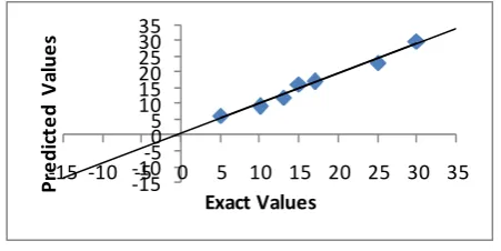
Table 1 shows the minimum and maximum error between exact values and predicted values of unseen days so that the generalization capacity of network can be checked after training and testing phase.
-15 -10-5 0 5 10 15 20 25 30 35
-15 -10 -5 0 5 10 15 20 25 30 35
P
re
d
ic
te
d
V
al
u
e
s
Exact Values
Fig 3: Comparison between exact and predicted values for unseen day
The exact and predicted values for each unseen days by the proposed technique is shown in Fig. 3. From the result shown in Fig. 2, Fig. 3 and Table 1, it is observed that the predicted values are in good agreement with exact values and the predicted error is very less. Therefore the proposed BPNN model with the developed structure can perform good prediction with least error.
V. CONCLUSION
In this paper, back propagation neural network is used for predicting the temperature based on the training set provided to the neural network. Through the implementation of this system, it is illustrated, how an intelligent system can be efficiently integrated with a neural network prediction model to predict the temperature. This algorithm improves convergence and damps the oscillations. This method proves to be a simplified conjugate gradient method. When
incorporated into the software tool the performance of the back propagation neural network was satisfactory as there were not substantial number of errors in categorizing. Back propagation neural network approach for temperature forecasting is capable of yielding good results and can be considered as an alternative to traditional meteorological approaches. This approach is able to determine the non-linear relationship that exists between the historical data (temperature, wind speed, humidity, etc.,) supplied to the system during the training phase and on that basis, make a prediction of what the temperature would be in future.
REFERENCES
[1] Xinghuo Yu, M. Onder Efe, and Okyay Kaynak,” A General Back propagation Algorithm for Feedforward Neural Networks Learning,” [2] R. Rojas: Neural Networks, Springer-Verlag, Berlin, 1996.
[3] Y.Radhika and M.Shashi,” Atmospheric Temperature Prediction using Support Vector Machines,” International Journal of Computer Theory and Engineering, Vol. 1, No. 1, April 2009 1793-8201. [4] M. Ali Akcayol, Can Cinar, Artificial neural network based modeling
of heated catalytic converter performance, Applied Thermal Engineering 25 (2005) 2341-2350.
[5] Mohsen Hayati, and Zahra Mohebi,” Application of Artificial Neural Networks for Temperature Forecasting,” World Academy of Science, Engineering and Technology 28 2007.
[6] Brian A. Smith, Ronald W. McClendon, and Gerrit Hoogenboom,” Improving Air Temperature Prediction with Artificial Neural Networks” International Journal of Computational Intelligence 3;3 2007.
[7] Arvind Sharma, Prof. Manish Manoria,” A Weather Forecasting System using concept of Soft Computing,”pp.12-20 (2006) [8] Ajith Abraham1, Ninan Sajith Philip2, Baikunth Nath3, P.
Saratchandran4,” Performance Analysis of Connectionist Paradigms for Modeling Chaotic Behavior of Stock Indices,”
[9] Surajit Chattopadhyay,” Multilayered feed forward Artificial Neural Network model to predict the average summer-monsoon rainfall in India ,” 2006
[10] Raúl Rojas,”The back propagation algorithm of Neural Networks - A Systematic Introduction, “chapter 7,ISBN 978-3540605058 [11] Mike O'Neill,” Neural Network for Recognition of Handwritten
Digits,” Standard Reference Data Program National Institute of Standards and Technology.
[12] Carpenter, G. and Grossberg, S. (1998) in Adaptive Resonance Theory (ART), The Handbook of Brain Theory and Neural Networks, (ed. M.A. Arbib), MIT Press, Cambridge, MA, (pp. 79–82). [13] Ping Chang and Jeng-Shong Shih,” The Application of Back
Propagation Neural Network of Multi-channel Piezoelectric Quartz Crystal Sensor for Mixed Organic Vapours,” Tamkang Journal of Science and Engineering, Vol. 5, No. 4, pp. 209-217 (2002). [14] S. Anna Durai, and E. Anna Saro,” Image Compression with
Back-Propagation Neural Network using Cumulative Distribution Function,” World Academy of Science, Engineering and Technology 17 2006.
[15] Mark Pethick, Michael Liddle, Paul Werstein, and Zhiyi Huang,” Parallelization of a Backpropagation Neural Network on a Cluster Computer,”
[16] K.M. Neaupane, S.H. Achet,”Use of backpropagation neural network for landslide monitoring,”Engineering Geology 74 (2004) 213–226. [17] http://www.wunderground.com/history/airport/VABB/2005/3/27/Cust
omHistory.html?dayend=27&monthend=3&yearend=2006&req_city =NA&req_state=NA&req_statename=NA
[18] Grossberg, S ,”Adaptive Pattern Classification and Universal Recoding: Parallel Development and Coding of Neural Feature Detectors”, Biological Cybernetics, 23, 121–134 (1976).
[19] Maurizio Bevilacqua, “Failure rate prediction with artificial neural networks,” Journal of Quality in Maintenance Engineering Vol. 11 No. 3, 2005 pp. 279-294Emerald Group Publishing Limited 1355-2511 [20] Chowdhury A and Mhasawade S V (1991), "Variations in
Meteorological Floods during Summer Monsoon Over India", Mausam, 42, 2, pp. 167-170.
326 Lt. Dr. S. Santhosh Baboo, aged forty three, has around Nineteen years of postgraduate teaching experience in Computer Science, which includes Six years of administrative experience. He is a member, board of studies, in several autonomous colleges, and designs the curriculum of undergraduate and postgraduate programmes. He is a consultant for starting new courses, setting up computer labs, and recruiting lecturers for many colleges. Equipped with a Masters degree in Computer Science and a Doctorate in Computer Science, he is a visiting faculty to IT companies. It is customary to see him at several national/international conferences and training programmes, both as a participant and as a resource person. He has been keenly involved in organizing training programmes for students and faculty members. His good rapport with the IT companies has been instrumental in on/off campus interviews, and has helped the post graduate students to get real time projects. He has also guided many such live projects. Lt. Dr. Santhosh Baboo has authored a commendable number of research papers in international/national Conference/journals and also guides research scholars in Computer Science. Currently he is Senior Lecturer in the Postgraduate and Research department of Computer Science at Dwaraka Doss Goverdhan Doss Vaishnav College (accredited at „A‟ grade by NAAC), one of the premier institutions in Chennai.
I. Kadar Shereef, done his Under-Graduation