Available at http://www.ijcsonline.com/
Evidence Informed Performance Modelling of Complex Business Process using
Queuing Petri Net (QPN)
Ravi Kumar Gedela, Kamakshi Prasad Valurouthu
Department of Computer Science Engineering, JNTU, Hyderabad, Andhra Pradesh-500 085, India
Abstract
Ideas are many, strategies are plenty, but how to connect to and align with profitability? Lots of potential and markets trends are ever more fluid. How do executives transform the legacy mainframe based system to enhance customer experience? Amongst numerous competitors, predictability stands out, and especially as Enterprise Services based Architecture has become de-facto architecture in the industry. Challenges are abound during the transformation journey – delivery, operational, functional and non-functional. The focus of this paper is to address performance prediction concerns in advance. As performance is one of the critical factors to provide better customer experience. This paper high lights evidence informed performance prediction of the complex business process using QPME (Queuing Petri Net Modelling Environment), which is a performance modelling and analysis tool. QPME is made of two components: QPE (QPN Editor) and SimQPN (Simulator for QPNs). We modeled the BPEL process description and transform it into QPN model. After that, we use the simulation tool SimQPN to analyze the model and suggested the recommendations. Order management business process is considered as part of the research work.
Keywords: Performance, SOA, QoS, BPEL, QPME (Queuing Petri Net Modelling Environment), software architecture.
I. INTRODUCTION
Exceptional organizations will do exceptionally well in the market place due to their commitment to the world of innovation. In distributed computing world, SOA has emerged as a new paradigm for modeling the process which allows efficient development applications. Despite of several advantages of SOA, the industry is still facing challenges of solutions addressing non-functional requirements, specifically performance. The performance of customer facing application has a direct impact to the operational efficiency of the organization and so as customer centricity. Therefore, the ability to assess the performance of SOA applications with different workloads is of great importance.
Performance of a SOA application depends on several factors,– a) the design of business process model (BPEL) built with business services b) underlying infrastructure including operating system c) middleware components and d) its tuning parameters. There are many SOA vendor specific business modeling tools which are available to model the business process and simulate the business model for predicting or evaluating business performance in business domain, however, they fail to meet requirements of performance modelling of business process (BPEL) in complex IT domain. In the IT domain, there is a need to model the business process performance for underlying agile hardware and software resource contentions. Our exhaustive research reveals that any insufficiently configured hardware resources such as memory size, number of CPUs, number of disks and software resources such as threads, processes and database connection pool size, business logic implemented component pool size, causes to severely impact the response time and throughput of the system.
The paper is organized in 3 parts. We first began with the details of the Order management business process, analysis, process steps and associated real world implementation details to set the context. The second part describes brief literature on performance modelling and methodology and introduced Queuing Petri Nets and SimQPN. The third part explains the how we have transformed the real-world BPEL process description into QPN model to predict the performance and conducted the experimentation and presented the results and conclusions.
II. ANALYSIS OF ORDER MANAGEMENT BUSINESS PROCESS
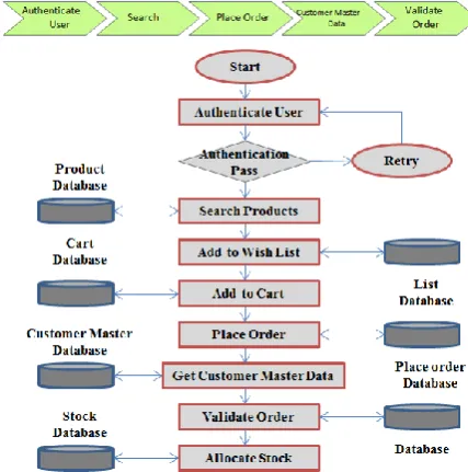
Order management process is long and complex process involving a large number of activities including system-to-system and system-to-human interactions. The business process is realized when the activities in the process invoke the underlying business services which are implemented by the business applications like order management application or payment gateway or accounting system. These business services are implemented using web services. A snap shot of the steps in the business process flow and how each activity uses the database is illustrated in figure 1. Most of the services are implemented by the Order Management application. The flow is as follows:
- Customer logs-in to the portal
- If authenticated the customer goes to next step
- The customer can search for products
- Customer can selected products to Wish List
- Customer also has an option to place order of the selected products
- Invocation of place order will result in the system to fetch customer master
- The system will then validate the order; makes checks like credit limit, availability and so on
- System can then go to payment process
The traditional SOA applications are built in Java and Microsoft .NET platform. The Middleware platforms are used for integration and common services. Application logic is normally partitioned into services distributed over physical tiers.
Figure 1 – Order Management Process flow
Figure 2 shows a typical architecture of a multi-tiered SOA application. There are n tiers: consumer tier, business process tier, services tier, application tier, integration tier, infrastructure tier, data tier. The consumer tier is responsible for interacting with different types of customers on multiple channels and could include includes Web portals that implement the presentation logic of the application. The business logic tier includes a cluster of application servers hosting business process tier provides business services which are consumed by the presentation or consumer tier, business process tier leverages the services provided the services tier. An integration tier is used to integrate the applications which are used by the business process tier while invoking services. The data tier includes database servers and legacy systems providing data management services. Web routers and load balancers are used to distribute incoming requests over the available Web servers and application servers, respectively. The inherent complexity of such architectures makes it extremely difficult to manage the end-to-end system Performance and Scalability. System architects are often confronted, in most projects, with the following questions during the various stages of the system life cycle:
- Identification and Selection of hardware platform considering application non-functional requirements (type of servers, disk subsystems, load balancers, etc.)
- Identification and selection of software platform, considering the organizational strategic initiatives, to make optimal decision (Operating Systems, middleware, databases, etc.) would provide the best scalability and cost/performance ratio for the application?
- Deployment considerations for best utilization of hardware and corresponding tuning parameters of the platforms selected to obtain the desired overall system performance?
- Is the current system design scalable? Which system components would be most utilized as the load increases and are there any potential bottlenecks?
- What maximum load would the system be able to handle in its current state without breaking the Service Level Agreements?
- What performance would the system exhibit for a given workload and configuration scenario?
- What would be the average transaction throughput and response time? How utilized would be the various system components (Web servers, application servers, database servers, etc.)?
- Which system components have the greatest effect on the overall system performance and how much would performance improve if they are optimized?
- How much hardware would be needed to guarantee that SLAs are met? How many Web servers, application servers and database servers would be required?
Internet
Internet
Customer
Web Server
Web Server Process Server – BPEL EngineProcess Server – BPEL Engine
Search
Search
Order Management
Order Management
Database
Database
Enterprise Service Bus
Enterprise Service Bus
Figure 2: Implementation of Order Management Business Process – a sub-process is chosen here for illustration of performance modelling
Figure 2 illustrates the flow of customer requests. The flow can be described as follows:
order, payment, and so on. All these requests are on http (hypertext transport protocol)
- Customer requests arrive at the load balancer. The load balancer based on the current load will route the request to the appropriate web server.
- The number of threads that has been configured on the web server determines the number of concurrent requests that it can handle and the additional requests will be queued.
- The web server forwards the customer request to the process server. The order management process will be exposed as a web service which will be invoked from the web server.
- The process server implements the BPEL process and uses the enterprise service bus (ESB). ESB will bind the request to the appropriate service from the underlying business applications
- The results of the invocation of business services will then be routed back to the customer as a http response
III. QUALITY OF SERVICE (QOS) OF BUSINESS PROCESS Legacy applications are the back bone for the financial enterprises as the core business is running on those applications and transformation of these applications are necessary to continue to be in business [5]. When the legacy transformation initiatives are mandated by the business, it is very critical that the foundation of SOA architecture must be done right. In the past, business process flows were typically embedded in software components and user interfaces. The SOA Reference Architecture (SOA RA) recognizes the promise of SOA and the challenges in the past in the ability to change the business processes as market changes and therefore introduces a specific layer for business processes and flows. The layer is called the Business Process Layer and allows externalization of the business process flow in a separate layer in the architecture and thus has a better chance to rapidly change as the market condition changes [6].
The Business Process Layer covers process and composition, and provides building blocks for aggregating loosely-coupled services. Data flow and control flow are used to enable interactions between services and business processes. The interaction may exist within an enterprise or across multiple enterprises. The business logic is used to form service flow as parallel tasks or sequential tasks based on business rules, policies, and other business requirements.
Any organizational business is realized in terms of business process, which will be implemented using business services. In particular, compositions of services exposed in the Services Layer are defined in this layer: atomic services are composed into a set of composite services using a service composition engine. Note that composition can be implemented as choreography of services or an orchestration of the underlying service elements.
Services combined or composed into flows or, for example, choreographies of services, bundled into a flow,
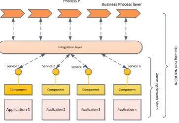
work together to establish an application. These applications support specific use-cases and business processes. Typically, a visual flow composition tool will be used to design the application flow. Services Orchestration shows how a Business Process “P” as shown in figure 3 can be implemented using Services 1, 2, 3, and n from the Services Layer. Process P contains the logic for the sequence in which the services need to be invoked and executed, as well as having responsibility for many of the non-functional aspects such as performance, scalability, security and so on. The services that are aggregated into a business process can be sourced from individual services or composite services [6]. This transition from traditional computer based systems to a service-oriented paradigm, the high-performance requirements of service-oriented critical systems remain the same.
There are many performance evaluation techniques are available, however Queueing Networks, Stochastic Petri Nets, Queueing Petri Nets are most widely used in research. The following section briefly explains the Queueing Networks but the focus of this paper is on Queueing Petri Nets.
Integration layer
Component Component Component Component
Application 1 Application 2 Application 3 Application n Process P
Business Process layer
Service 1 Service 2 Service 3 Service n
Q
u
eu
ein
g N
et
w
o
rk
M
o
d
el
Q
u
eu
ein
g P
et
ri N
et
s (Q
P
N
)
Figure 3 (a) – Service Orchestration for Business Process implementation modelled as Queueing Petri nets (QPN)
Figure 3(b) – Layered Queueing model of the services layer
IV. OVERVIEW OF QUEUING PETRI NETS MODELLING ENVIRONMENT AND SIMQPN
QPME (Queuing Petri Net Modelling Environment) is a performance modelling environment based on the Queuing Petri Net (QPN) modelling formalism. QPN formalism has a number of advantages over conventional modelling formalisms such as queuing networks and stochastic Petri nets. By combining the modelling power and expressiveness of queuing networks and stochastic Petri nets, Queuing Petri Nets (QPNs) enable the integration of hardware and software aspects of system behavior into the same model [1]. In [3], we showed how this advantage can be exploited for modelling distributed e-business applications. However, while the QPN modelling paradigm provides many important benefits, there are currently few tools that support the modelling and analysis of systems using QPNs.
QPE (Queuing Petri Net Editor), the first major component of QPME, provides a graphical tool for modelling using QPNs [7]. It offers a user-friendly interface enabling the user to quickly and easily construct QPN models. QPE is based on the model-view-controller (MVC) architecture. The model in our case is the QPN being defined, the views provide graphical representations of the QPN, and finally the controller connects the model with the views, managing the interactions among them.
A characterizing feature of QPE is that it allows token colors to be defined globally for the whole QPN instead of on a per place basis. This feature was motivated by the fact that in QPNs typically the same token color (type) is used in multiple places. Instead of having to define the color multiple times, the user can define it one time and then reference it in all places where it is used. This saves time, makes the model definition more compact, and last but not least, it makes the modelling process less error-prone since references to the same token color are specified explicitly.
The second major component of QPME is SimQPN – a discrete-event simulation engine specialized for QPNs. SimQPN simulates QPNs using a sequential algorithm based on the event-scheduling approach for simulation modeling. Being specialized for QPNs, it simulates QPN models directly and has been designed to exploit the knowledge of the structure and behavior of QPNs to improve the efficiency of the simulation. Therefore, SimQPN provides much better performance than a general purpose simulator would provide, both in terms of the speed of simulation and the quality of output data provided. SimQPN currently supports three different scheduling strategies for queues inside queuing places: First-Come-First-Served (FCFS), Processor-Sharing (PS) and Infinite Server (IS). A wide range of service time distributions are supported including Beta, Breit-Wigner, Chi-Square, Gamma, Hyperbolic, Exponential, ExponentialPower, Logarithmic, Normal, StudentT, Uniform, VonMises and Empirical. Timed transitions are currently not supported, however, in most cases a timed transition can be approximated by a serial network consisting of an immediate transition, a queuing place and a second immediate transition.
SimQPN offers the ability to configure what data exactly to collect during the simulation and what statistics to provide at the end of the run. This can be specified for each place (ordinary or queuing) of the QPN. The user can choose one of four modes of data collection. The higher the mode, the more information is collected and the more statistics are provided. Since collecting data costs CPU time, the more data is collected, the slower the simulation would run. Therefore, by configuring data collection modes, the user can make sure that no time is wasted collecting unnecessary data and, in this way, speed up the simulation. SimQPN supports two methods for estimation of the steady state mean residence times of tokens inside the queues, places and depositories of the QPN. These are the well-known method of independent replications (in its variant referred to as replication/deletion approach) and the classical method of non-overlapping batch means. Both of them can be used to provide point and interval estimates of the steady state mean token residence time. The method of Welch is used for determining the length of the initial transient (warm-up period). A novel feature of SimQPN is the introduction of the so-called departure disciplines. The latter are defined for ordinary places or depositories and determine the order in which arriving tokens become available for output transitions. We define two departure disciplines, Normal (used by default) and First-In-First-Out (FIFO). The former implies that tokens become available for output transitions immediately upon arrival just like in conventional QPN models. The latter implies that tokens become available for output transitions in the order of their arrival, i.e. a token can leave the place/depository only after all tokens that have arrived before it have left, hence the term FIFO [4].
V. PERFORMANCE MODELLING METHODOLOGY We have adopted performance modelling methodology suggested by Samuel Kounev [2] to conduct the performance modelling of order management business process, a complex process which has several integration points with other third party systems:
VI. QPN MODEL OF BUSINESS PROCESS A number of different modelling formalisms have been developed in the past decades that can be used for modelling component based systems. Queueing Networks (QNs) and Stochastic Petri Nets (SPNs) are perhaps the two most popular types of models that have been exploited in practical studies. However, they both have some serious shortcomings. While QNs provide a very powerful mechanism for modelling hardware contention and scheduling strategies, they are not as suitable for representing blocking and synchronization of processes. SPNs, on the other hand, lend themselves well to modelling blocking and synchronization aspects, but have difficulty in representing scheduling strategies. A modelling formalism called Queueing Petri Nets (QPNs) combines QNs and SPNs into a single formalism and eliminates the above disadvantages. QPNs allow queues to be integrated into places of Petri nets. This enables the modeler to easily represent scheduling strategies and brings the benefits of QNs into the world of Petri nets.
The motivation for this modelling exercise is the Order management business process that we have discussed earlier. The approach that we have adopted in designing the QPN model is based on the directions provided by the developer of QPME tool and illustrated in [2]. The first step to modelling is to understand the workload characterization that we briefly touched upon in the previous chapter. The following workload classes were identified:
- Browse
- Search (for Products)
- Order (for Products)
- Payment
Figure 4.3 illustrates the tokens or colors selected for each type of transactions – “B” for “Browse”, “S” for “Search”, “O” for “Order”, and “P” for “Payment”. The sub-transaction for each transaction is also shown in figure 4.3. There could be a set of sub-transaction for each transaction. In order to make the performance model more compact, it is assumed that each server used during processing of a sub-transaction is visited only once and that the sub-transaction receives all of its service demands at the server’s resources during that single visit. This simplification is typical for queuing models and has been widely employed. Similarly, during the service of a sub-transaction at a server, for each server resource used (e.g., CPUs, disk drives), it is assumed that the latter is visited only one time, receiving the whole service demand of the sub-transaction at once. These simplifications make it easier to model the flow of control during processing of sub-transactions. The assumption is, while characterizing the workload service demands the total service demand of a transaction at a given system resource is spread evenly over its transactions. This allows us to consider the sub-transactions of a given workload class as equivalent in terms of processing behaviour and resource consumption. Thus, we can model sub-transactions using a single token type (color) per workload class as follows: “b” for “Browse”, “s” for search, “o” for “order” , “p” for “payment” sub- transaction at once.
Figure 4.3 – A screen shot of Colors (tokens) for each type of transaction
These simplifications make it easier Business process management built on top of web services has become an important research subject. In this work we transform the basic BPEL structure to QPN model. In this work a QPN model is designed to analyze the performance of web services. Figure 4.4 illustrates the QPN model of order
management process.
-Figure 4.4- QPN Model of Order Management Process steps.
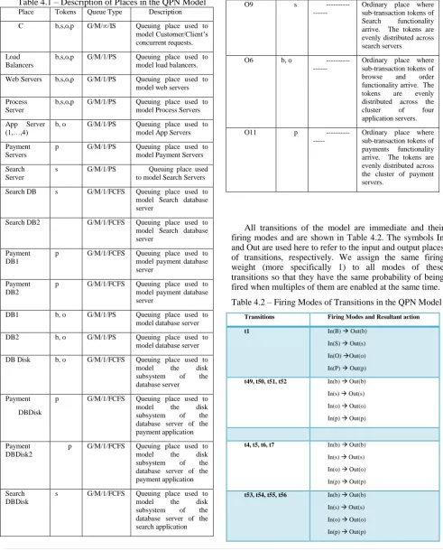
service at the application server CPU, the sub-transaction token is moved to place from where it is sent to database server CPUs and database disks with equal probability. Similarly, when a payment sub-transaction is sent to the process server it routes the request to payment application servers. All token service times at the queues of the model are assumed to be exponentially distributed. The table 4.1 provides description of the places in the QPN model used for modelling order management process.
Table 4.1 – Description of Places in the QPN Model Place Tokens Queue Type Description
C b,s,o,p G/M/∞/IS Queuing place used to model Customer/Client’s concurrent requests.
Load Balancers
b,s,o,p G/M/1/PS Queuing place used to model load balancers.
Web Servers b,s,o,p G/M/1/PS Queuing place used to model web servers
Process Server
b,s,o,p G/M/1/PS Queuing place used to model Process Servers
App Server
(1,…,4) b, o G/M/1/PS Queuing place used to model App Servers
Payment Servers
p G/M/1/PS Queuing place used to model Payment Servers
Search Server
s G/M/1/PS Queuing place used to model Search Servers
Search DB s G/M/1/FCFS Queuing place used to model Search database server
Search DB2 G/M/1/FCFS Queuing place used to model Search database server
Payment DB1
p G/M/1/FCFS Queuing place used to model payment database server
Payment DB2
p G/M/1/FCFS Queuing place used to model payment database server
DB1 b, o G/M/1/PS Queuing place used to model database server
DB2 b, o G/M/1/PS Queuing place used to model database server
DB Disk b, o G/M/1/FCFS Queuing place used to model the disk subsystem of the database server
Payment
DBDisk
p G/M/1/FCFS Queuing place used to model the disk subsystem of the database server of the payment application
Payment DBDisk2
p G/M/1/FCFS Queuing place used to model the disk subsystem of the database server of the payment application
Search DBDisk
s G/M/1/FCFS Queuing place used to model the disk subsystem of the database server of the search application
O12, O13, O14, O15, O4,
b,s,o,p ---
Ordinary places where sub-transaction tokens arrive. These places are used to design the clusters. The sub-transaction tokens that arrive in these places will be evenly distributed between the CPUs of the queuing place
O9 s
---
Ordinary place where sub-transaction tokens of Search functionality arrive. The tokens are evenly distributed across search servers
O6 b, o ---
Ordinary place where sub-transaction tokens of browse and order functionality arrive. The tokens are evenly distributed across the cluster of four application servers.
O11 p
---
Ordinary place where sub-transaction tokens of payments functionality arrive. The tokens are evenly distributed across the cluster of payment servers.
All transitions of the model are immediate and their firing modes and are shown in Table 4.2. The symbols In and Out are used here to refer to the input and output places of transitions, respectively. We assign the same firing weight (more specifically 1) to all modes of these transitions so that they have the same probability of being fired when multiples of them are enabled at the same time. Table 4.2 – Firing Modes of Transitions in the QPN Model
Transitions Firing Modes and Resultant action
t1 In(B) Out(b)
In(S) Out(s)
In(O) Out(o)
In(P) Out(p)
t49, t50, t51, t52 In(b) Out(b)
In(s) Out(s)
In(o) Out(o)
In(p) Out(p)
t4, t5, t6, t7 In(b) Out(b)
In(s) Out(s)
In(o) Out(o)
In(p) Out(p)
t53, t54, t55, t56 In(b) Out(b)
In(s) Out(s)
In(o) Out(o)
t12, t13, t14, t15, t16, t17, t18, t19
In(b) Out(b)
In(o) Out(o)
t32, t33, t57, t58 In(b) Out(b)
In(o) Out(o)
t42, t43, t23, t25 In(s) Out(s
t61, t62, t44, t36 In(s) Out(s)
t37 In(s) Out(s)
t45, t46, t47, t34 In(p) Out(p)
t59, t60, t48, t35 In(p) Out(p)
t39 In(p) Out(p)
The workload intensity and service demand parameters are used to provide values for the service times of tokens at the various queues of the model. A separate set of parameter values is specified for each workload scenario considered. The service times of sub-transactions at the queues of the model are estimated by dividing the total service demands of the respective transactions by the number of sub-transactions they have [2].
VII. DISCUSSION ON RESULTS
As part of the experimentation, we carried out modelling and simulation for three different scenarios:
1.Architecture with Server clusters for Order management business process for low load 2.Architecture with Server clusters for Order
Management business process for high load (300% of low load)
To prove the model validity we conducted performance tests on physical servers and obtained metrics like throughput, utilization and response times. These metrics were measured only for Search and Payment transactions. The idea is to validate the model and refine it if required. The applications were deployed on JBOSS Application server running on Windows and Intel boxes and the database servers were oracle database running windows-Intel boxes.
A. Low Load Scenario
The concurrent users for each of these transactions - B = 40; S = 20; O = 25; P = 20.
After the model is built in QPME (Queueing Petri Nets Modelling Environment) the model needs to be simulated for which we use SimQPN tool. SimQPN simulates QPNs based on the event-scheduling approach to simulation modelling. Being specialized for QPNs, it simulates QPN models directly and has been designed to exploit the knowledge of the structure and behavior of QPNs to improve the efficiency of the simulation. Therefore, SimQPN provides much better performance than a general purpose simulator would provide, both in terms of the speed of simulation and the quality of output data provided. Here we use the method of non-overlapping batch means for steady state analysis. The results from the simulation which are used for performance prediction will be
compared with actual measurements to validate the model. Only a few scenarios will be compared with actual measurements.
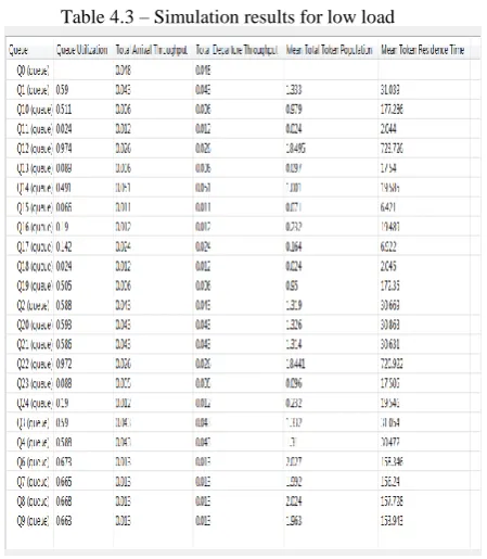
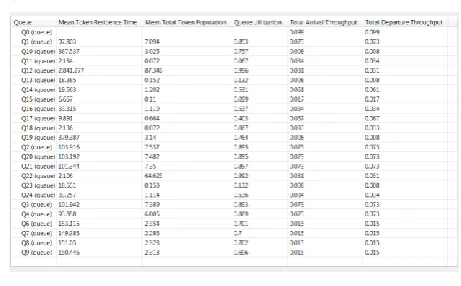
Performance analysis of BPM/SOA always considers the following several performance indicators: mean token residence time, queue utilization and mean token population.
The results from the model is shown in table 4.3 Table 4.3 – Simulation results for low load
Comparisons of the simulated results with actual measurements are shown in Table 4.4. This kind of table is not there for 2 and 3.
Table 4.4 – Comparison of Simulation results with Actual Measurements
MET RIC
MODEL (%)
MEASURE D (%)
ERRO R (%)
TP 0.6 0.585 2.6
TS 1.2 1.18 1.7
UP 51.1 50.4 1.4
US 2.4 2.35 2.1
(TP – Throughput of Payment Server; TS – Throughput of Search Server; UP – Utilization of payment Server; US – Utilization of Search Server)
B. High Load Scenario
The concurrent users for each of these transactions - B – 120; S – 60; O – 75; P – 60
In this scenario, we repeat the simulation with higher values of concurrent users. Here we subject the model to an increase of 300% in concurrent users from low load values. The measurements from simulation is given in Table 4.5
Table 4.5 - Simulation results for High load (300% of Low load)
VIII. CONCLUSIONS AND FUTURE WORK In this paper, we have presented the real-world in depth Order Management business process analysis and outlined the complexity and how performance prediction can be done in the early stages of the implementation using Queueing petri Nets. The developed model is tested against multiple scenarios to test accuracy. We also have conducted the real world implementation of the same process, tested and compared the results with the modeled ones. The results reveal that the modeled and measured results are very close and the gap can be filled by tuning the different parameters. We have also used the standard performance methodology, outlined Samuel Kounev by for modelling and evaluating the real-world business process in the early stages of life cycle.
Also, we have chosen the complex and non-trivial order management business process for modelling and performance prediction. Critical steps in the entire process are selected to carry performance modelling using Queuing petri nets. By subjecting the QPN model developed to various workloads, scalability is sustained up to 300% of the normal load while agility is with acceptable range. As the model followed an enterprise class design, adopted best practices and patterns it supported scalability very well. The same business process when modeled natively exhibited severe performance and scalability bottlenecks.
Digital transformation exercise is been happening in most of the enterprises. BPM/SOA applications are nowadays hosted on virtualized environments and Cloud platforms, therefore there is a need to explore how QPN formalism is suited for these environments and if need be how to extend the formalisms to cover these platforms. With the advent of Big Data, we would like to explore to see how to use QPN formalisms to address the performance concerns with for Hadoop clusters and NO SQL databases.
ACKNOWLEDGMENT
Our sincere thanks to Nataraj Venkataraman, who has been constantly providing from innovative ideas and suggestions while conducting this research.
.
REFERENCES
[1] F. Bause, P. Buchholz, and P. Kemper, “Integrating Software and Hardware Performance Models Using Hierarchical Queueing Petri Nets,” in Proceedings of the 9. ITG / GI - Fachtagung Messung, Modellierung und Bewertung von Rechen- und Kommunikations systemen, (MMB’97), Freiberg (Germany), 1997.
[2] S. Kounev. Performance Modeling and Evaluation of Distributed Component-Based Systems using Queueing Petri Nets. IEEE Transactions on Software Engineering, 32(7):486-502, July 2006 [3] S. Kounev and A. Buchmann. Performance Modeling of Distributed
E-Business Applications using Queueing Petri Nets. In Proceedings of the 2003 IEEE International Symposium on Performance Analysis of Systems and Software (ISPASS 2003), Austin, Texas, USA, March 6-8, 2003, pages 143-155, Washington, DC, USA, 2003. IEEE Computer Society
[4] S. Kounev, Christofer Dutz, Alejandro Buchmann, QPME - Queueing Petri Net Modeling Environment, Third International Conference on the Quantitative Evaluation of Systems (QEST'06), IEEE, 2006
[5] Ravi K Gedela et.al – Maximizing the business value from Silos- Service based transformation with Service data models , IEEE (2011)